Comparative Analysis of Traditional and Modified DECODE Method in Small Sample Gene Expression Experiments

(1)

COMPARATIVE ANALYSIS OF TRADITIONAL AND MODIFIED DECODE METHOD IN SMALL SAMPLE GENE EXPRESSION EXPERIMENTS

A Thesis

Submitted to the Graduate Faculty of the

North Dakota State University of Agriculture and Applied Science

By Katie Jean Neset

In Partial Fulfillment of the Requirements for the Degree of

MASTER OF SCIENCE

Major Department: Statistics

(2)

North Dakota State University

Graduate School

Title

COMPARATIVE ANALYSIS OF TRADITIONAL AND MODERATED DECODE METHOD IN SMALL SAMPLE GENE EXPRESSION

EXPERIMENTS

By

Katie Jean Neset

The Supervisory Committee certifies that this thesis complies with North Dakota State University’s regulations and meets the accepted standards for the degree of

_{MASTER OF SCIENCE} SUPERVISORY COMMITTEE: Dr. Megan Orr Chair Dr. Ron Degges Dr. Anne Denton Approved:

April 10, 2018 Dr. Rhonda Magel

(3)

ABSTRACT

Background: The DECODE method integrates differential co-expression and differential expression analysis methods to better understand biological functions of genes and their

associations with disease. The DECODE method originally was designed to analyze large sample gene expression experiments, however most gene expression experiments consist of small sample sizes. This paper proposes modified test statistic to replace the traditional test statistic in the DECODE method. Using three simulations studies, we compare the performances of the modified and traditional DECODE methods using measures of sensitivity, positive

predictive value (PPV), false discovery rate (FDR), and overall error rate for genes found to be highly differentially expressed and highly differentially co-expressed.

Results: In comparison of sensitivity and PPV a minor increase is seen when using modified DECODE method along with minor decrease in FDR and overall error rate. Thus, a recommendation is made to use the modified DECODE method with small sample sizes.

(4)

TABLE OF CONTENTS

ABSTRACT ... iii

LIST OF TABLES ... vi

LIST OF FIGURES ... vii

LIST OF ABBREVIATIONS ... viii

LIST OF APPENDIX TABLES ... ix

CHAPTER 1. INTRODUCTION ... 1

CHAPTER 2. LITERATURE REVIEW ... 3

2.1. Differential Expression ... 3

2.2. Differential Co-Expression ... 5

CHAPTER 3. METHODOLOGY ... 8

3.1. DECODE Method ... 8

3.1.1. Phase One: Test Statistics ... 8

3.1.2. Phase Two: Partition Creation ... 10

3.1.3. Working Example ... 11

3.2. Moderated Approach ... 13

3.3. Simulations ... 14

3.3.1. Normal Simulations ... 17

3.3.2. Microarray Simulations ... 20

3.3.2.1. Microarray Simulations (Breast Cancer) ... 20

3.3.2.2. Microarray Simulations (Psoriatic) ... 21

CHAPTER 4. RESULTS ... 22

(5)

4.3. Psoriatic Simulation Results ... 31

CHAPTER 5. CONCLUSION AND DISCUSSION ... 35

5.1. Conclusion ... 35 5.2. Recommendations ... 36 5.3. Future Work ... 36 REFERENCES ... 37 APPENDIX. TABLES ... 39

(6)

LIST OF TABLES

Table Page

3.1. Gene Partition Contingency Table ... 11

3.2. Working Example DE and DC Test Statistics (Threshold Possibilities) ... 12

3.3. Partition Contingency Table for Gene 1 using Gene 2 Thresholds ... 13

3.4. Correct HE/HC Values for Population and Sample Results (Notation Example) ... 16

(7)

LIST OF FIGURES

Figure Page

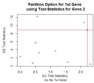
3.1. Working Example Partitions for Gene 1 using Gene 2 Thresholds Graphic

Example ... 12 4.1. Average Sensitivity Values by Sample Size (4-20) by Test Statistic for Normal

Simulations ... 23 4.2. Average FDR Values by Sample Size (4-20) by Test Statistic for Normal

Simulations ... 25 4.3. Average Overall Error Rate Values by Sample Size (4-20) by Test Statistic for

Normal Simulations ... 26 4.4. Average Sensitivity Values by Sample Size by Test Statistic for Breast Cancer

Simulations ... 28 4.5. Average FDR Values by Sample Size by Test Statistic for Breast Cancer

Simulations ... 30 4.6. Average FDR Values by Sample Size by Test Statistic for Psoriatic Simulations ... 32 4.7. Average Sensitivity Values by Sample Size by Test Statistic for Psoriatic

Simulations ... 33 4.8. Average Overall Error Rate Values by Sample Size by Test Statistic for Psoriatic

(8)

LIST OF ABBREVIATIONS

PPV ...Positive Predictive Value FDR ...False Discovery Rate

DE ...Differential Expression/Differentially Expressed DC ...Differential Co-Expression/ Differentially

Co-Expressed

HE/HC ...High Differential Expression High Differential Co-Expression

HE/LC ...High Differential Expression Low Differential Co-Expression

LE/HC ...Low Differential Expression High Differential Co-Expression

LE/LC ...Low Differential Expression Low Differential Co-Expression

DECODE ...Differential Co-Expression and Differential Expression Method

(9)

LIST OF APPENDIX TABLES

Table Page

A1. DECODE Method with Traditional Test Statistic (Normal Simulations with 400

genes)……….…….………...39 A2. DECODE Method with Moderated Test Statistic (Normal Simulations with 400

genes)……….……….………...39 A3. DECODE Method with Traditional Test Statistic (Normal Simulations with 1000

genes)……….……….………...40 A4. DECODE Method with Moderated Test Statistic (Normal Simulations with 1000

genes)………...……….……….40 A5. DECODE Method with Traditional Test Statistic (Normal Simulations with 3000

genes)………...……….……….41 A6. DECODE Method with Moderated Test Statistic (Normal Simulations with 3000

genes)………...……….……….41 A7. DECODE Method with Traditional Test Statistic (Normal Simulations with 5000

genes)………...……….……….42 A8. DECODE Method with Moderated Test Statistic (Normal Simulations with 5000

genes)………...……….……….42 A9. DECODE Method with Traditional Test Statistic (Breast Cancer Simulations with

400 genes)……….………...……….43 A10. DECODE Method with Moderated Test Statistic (Breast Cancer Simulations with

400 genes)………...….……….…….43 A11. DECODE Method with Traditional Test Statistic (Breast Cancer Simulations with

(10)

A15. DECODE Method with Traditional Test Statistic (Breast Cancer Simulations with 5000 genes)………..………….….……....46 A16. DECODE Method with Moderated Test Statistic (Breast Cancer Simulations with

5000 genes)………...………..……..……...46 A17. DECODE Method with Traditional Test Statistic (Psoriatic Simulations with 400

genes)….………...……….47 A18. DECODE Method with Moderated Test Statistic (Psoriatic Simulations with 400

genes)………...……….………....….47 A19. DECODE Method with Traditional Test Statistic (Psoriatic Simulations with 1000

genes)….……….………..……….48 A20. DECODE Method with Moderated Test Statistic (Psoriatic Simulations with 1000

genes)……….……….……….………....…..48 A21. DECODE Method with Traditional Test Statistic (Psoriatic Simulations with 3000

genes)….……….………….………..49 A22. DECODE Method with Moderated Test Statistic (Psoriatic Simulations with 3000

genes)……….…….………….………....…..49 A23. DECODE Method with Traditional Test Statistic (Psoriatic Simulations with 5000

genes)….……….……….………..50 A24. DECODE Method with Moderated Test Statistic (Psoriatic Simulations with 5000

genes)……….……….……….………....…..50

(11)

CHAPTER 1.INTRODUCTION

Differential expression analysis has been extensively studied in the gene expression experiments. However the past decade has led to advances and a gain in popularity of differential co-expression analysis. Though there have been advances in the individual fields of differential expression and differential co-expression, there have been few methods that consider these two methods of analysis together. The DECODE method, Differential Co-Expression and

Differential Expression, was created by Thomas WH Lui et. al. to merge these two forms of gene expression analysis. The DECODE method is built to handle two condition studies, where one would be considered ‘normal’ state and the second would be the condition of interest referred to as the ‘disease’ state.

The original DECODE method was created to analyze large sample gene expression studies. However, an overview of the National Center for Biotechnology Information (NCBI) site shows that most gene expression studies have small samples (Gene Expression Omnibus, 2018). For this reason, we propose using the moderated test statistic to better estimate the variances in small sample gene expression studies (Smyth, 2004).

This paper will compare the performance of the DECODE method using the traditional test statistic and the moderated test statistic with the goal of determining if the moderated test statistic is advantageous for smaller samples. In order to determine if it the moderated test

(12)

This thesis is organized as follows. Chapter 2 provides an introduction to differential expression analysis and differential co-expression analysis. Chapter 3 provides the methodology of the DECODE method using the traditional test statistic and the moderated test statistic as well as a description of the simulation studies. Results from these simulations will be reported in Chapter 4 followed by the Conclusion and Discussion in Chapter 5.

(13)

CHAPTER 2.LITERATURE REVIEW 2.1.Differential Expression

Gene expression is the quantification of the ‘abundance’ of mRNA corresponding to a gene in an organism. An individual gene’s expression may change from cell to cell depending on the needs of the cell. For example if a cell is affected by a condition or disease, that cell may be in need of more or less mRNA from a particular gene.

In differential expression analysis, we seek to find a set of genes that are differentially expressed (DE) between two or more conditions. In many approaches, this involves performing a hypothesis test for each gene. For each test, the null hypothesis is that the gene is equivalently expressed (EE) i.e., that there is no difference in the average mRNA abundance between the conditions and the alternative hypothesis is that the gene is differentially expressed, i.e. that there is a difference in the average mRNA abundance levels between the conditions. If we fail to reject the null hypothesis, there is not enough evidence to conclude the gene is DE. If we reject the null hypothesis, there is enough evidence and the gene is declared to be differentially expressed (DDE). As with any hypothesis test, we are unable to say with complete confidence that that specific gene is truly DE even if it is DDE.

(14)

Many different methods have been proposed including parametric and nonparametric approaches. Traditional statistical methods can be applied to each gene in a gene expression experiment, such as the traditional t-test and F- test, to test for differential expression. However, with tens of thousands of genes being tested in a typical experiment, there needs to be a

correction on the resulting p-values in order to control multiple testing error. Methods used to control family-wise error rate include Bonferroni, Holm’s, and Scheffe (Bonferroni, 1936), (Holm, 1979), (Lindley, 1999). Methods used to control false discovery rate, the preferred multiple testing error to control in most gene expression studies include Benjamini and Hochberg, and q-values (Benjamini, 1995) (Storey, 2003). A common parametric method for differential expression is the moderated t test and is considered an improvement over the traditional t test (Smyth, 2004).

The moderated t test was created by Gordon K. Smyth et. al. with the goal of improved estimation of gene-wise variances. When sample sizes are small, the sample variance tends to be an unstable estimate of the population variance, resulting in an unreliable traditional t test

statistic. An assumption of the moderated t test approach is that the variances in gene expression differ from gene to gene, but follow an inverse gamma distribution. In order to estimate the parameters of this distribution, this approach uses empirical Bayesian methods to borrow information from all genes to better estimate the variance of an individual gene. More information on this method is provided in Chapter 3.

(15)

The parametric tests described above assume normality assumptions hold. When these assumptions are not met, nonparametric approaches can be applied as they do not assume normality. Some of the more common nonparametric methods are the Significance Analysis of Microarrays Method (SAM) (Tusher, 2001) and the Wilcoxon sum rank test (Troyanskaya, 2002). The SAM method is a permutation procedure in which the test statistic, similar to a traditional t-test statistic, is compared to the distribution of test statistics from permuted data sets. The Wilcoxon sum rank test determines if the sum of ranks of expressions from one condition is significantly higher or lower than what would be expected if the expression values from each condition come from the same distribution.

2.2.Differential Co-Expression

While differential expression has been around for the past two decades, the idea of looking of differential correlation is a newer topic in the field of gene expression. Differential correlation can also be referred to as differential co-expression while both denoted DC, which term to use is often left up to the author. We are going to consider two main ideas behind differential co-expression. The first was stated by de la Fuente A. that correlation between a set of given genes could affected by a given disease or treatment (de la Fuente, 2010). The second is that it is conceivable that genes are correlated due to a causational relationship.

(16)

In “Loss of Connectivity in Cancer Co-Expression Networks” Anglani et. al. found evidence to support the claim that abundance levels are not always effected in a way that can be seen by differential expression. This study found that there was a significant decrease in

correlation (Roberto A., 2014). This is considered evidence to support the first idea of differential co-expression, correlation can change for a given condition while not affecting abundance levels. More studies have also found evidence for this claim (Amar, 2013) (Watson, 2006).

The second main idea contemplates that two or more genes are correlated due to a causational relationship, also referred to as functional relationships. By locating these functional relationships, we are able to find another starting point in gene analysis. For example, Cho S. et. al. uses this idea in Identifying Set-Wise Differential Co-Expression in Gene Expression

Microarray Data to create differentially coexpressed genes sets algorithm (dCoxS) to find gene set pairs that have a causational relationship (Cho, 2009).

According to Wang et. al there are three different ways that DC can be represented. The first is referred to as the “shift”. When the shift takes places, the correlations of the genes are not affected however the expression levels are affected (i.e., they are DE). The second way DC can be represented is referred to as the cross. When a cross takes place genes may be positively correlated under one condition but negatively correlated under another condition. Finally there is the “re-wiring” where genes are either positively or negatively correlated under one condition but not correlated or less correlated under another condition (Wang, 2017).

(17)

One method that can be used to determine differential correlation is Bayes Factor to Differential Co-expression Analysis (BFDCA). The BFDCA method consists of five phase, one phase uses Bayes factors to determine highly correlated genes after discarding low Bayes factors values, the larger values are used to connected possible collaborating genes (Wang, 2017). Another method is used in ‘Find disease specific alterations in co-expression of genes’ where they created a score for differential co-expression. Using an additive model for each gene pair to get the corresponding differential co-expression score, they find a set of genes that are DC. A gene pair is declared to be DC when resulting in a low differential co-expression score (Kostka, 2004)

Another differential co-expression method that will be used in this thesis is the Z measure. From ‘differential expression’ to differential networking’- Identification of

Dysfunctional Regulatory Networks in Disease by de la Fuente A. et. al. considers the option to test if the correlation between two genes differs between two conditions. More detail on this formula will be found in 3.1.1. In order to use this method, there must be more than three

replicates per treatment group. This test statistic is considered more reliable when there are more than 10 replicates (de la Fuente, 2010). However all of these methods fail to consider differential expression along with differential co-expression.

(18)

CHAPTER 3.METHODOLGY 3.1.DECODE Method

The DECODE method, created by Lui et. al. combines two popular methods for analyzing gene expression data- differential expression analysis and differential co-expression analysis. The motivation behind this approach was to find a way to integrate these two methods to better understand how genes work together differently in different conditions. In order to integrate these two methods, each gene is classified as high or low differentially expressed and high or low differential co-expressed to create four different types of genes, referred to as partitions. The four partitions are low DE low DC (LE/LC), low DE high DC (LE/HC), high DE low DC (HE/LC), and high DE high DC (HE/HC). The DECODE method can be broken down into three steps: calculation of test statistics, partition creation, and evaluation of functional relevance. This thesis will focus on the first two steps.

It should be noted that there are two main technologies used to retrieve mRNA

abundance levels: microarray technology and RNA Next Generation (RNA-seq) technology. The DECODE method requires the use of microarray data. Microarray data is considered to be continuous versus RNA-seq data which produces count data. This thesis focuses on the analysis of microarray data.

3.1.1.Phase One: Test Statistics

The DECODE method begins by finding measures for differential expression and differential co-expression. A measure of differential expression is found for each gene by calculating the absolute value of a traditional t test statistic. That is, for a given gene 𝑖,

|𝑡𝑖| = |𝑥̅̅̅ − 𝑥_𝐷 ̅̅̅̅|_𝑁 √𝑠𝐷2 𝑛𝐷 + 𝑠_𝑁2 𝑛𝑁

(19)

where 𝑥̅ represents the average gene expression level, 𝑠2_{represents the sample gene expression} variance, the test statistics denoted N represent the normal sample and D represents the disease samples values, and lastly 𝑖 = 1 … 𝑚 and 𝑚 is the number of genes. Not that the direction of regulation (up or down) does not impact this measure. In order to find differential co-expression, the Z measure is used (de la Fuente, 2010). The first step in finding the Z measure is by

calculating the Pearson correlation coefficient for each pair of genes in each condition. Let r_ijN and rijD represents the normal (N) and the disease (D) state correlation coefficients respectively, between the ith and jth genes. Then the Fisher-transformation on these coefficients is performed, so that z_ijN_and_z

ijD are both assumed to be approximately normally distributed:

zijN = 1 2ln | 1 + r_ijN 1 − r_ijN| zijD = 1 2ln | 1 + r_ijD 1 − rijD|

We are now able to calculate the Z measure for genes 𝑖 and 𝑗 from𝑖 = 1 … 𝑚 and 𝑗 = 1 … 𝑚: Z_ij = |zij N_{− z} ijD| √ 1_n N− 3 + 1 nD− 3

It is important to note that to implement this method; the smallest possible sample size for each state is four.

(20)

3.1.2.Phase Two: Partition Creation

For each gene, the differential expression and differential co-expression test statistics are used to select thresholds for classifying genes as high or low DE and high or low DC. The thresholds are selected by maximizing the test statistic for Pearson’s Chi-Squared Test of Association for each gene 𝑗. Consider gene 𝑗. For each pair of threshold candidates, 𝑡_𝑖 and 𝑍_𝑖𝑗 , the genes are divided into the four partitions given the selected thresholds, the total. The total threshold candidates will be 𝑚, the number of genes. The four thresholds are defined as follows:

Low DE and Low DC (LE/LC) = { (t_k, z_kj), where z_kj< z_ij and t_k< t_i} High DE and Low DC (HE/LC) = { (t_k, z_kj), where z_kj< z_ij and t_k≥ t_i} Low DE and High DC (LE/HC) = { (t_k, z_kj), where z_kj≥ z_ij and t_k < t_i} High DE and High DC (HE/HC) = { (tk, zkj), where zkj≥ zij and tk≥ ti}

After partitioning all of the genes we are able to construct a two by two contingency table (Table 3.1.), which will be used to find the Pearson’s Chi-Squared Test statistic:

𝜒2 _{= ∑ ∑}(𝑚𝑖𝑗 − 𝜇𝑖𝑗)2 𝜇_𝑖𝑗 2 𝑗=1 2 𝑖=1 𝑎𝑛𝑑 𝜇_𝑖𝑗 =𝑚𝑖+𝑚+𝑗 𝑚 𝑓𝑜𝑟 𝑖 = 𝑗 = 1,2

where 𝑚𝑖𝑗 represents the observed genes in the partition, 𝑚𝑖𝑗 represents the partition mean, 𝑚𝑖+ represents the sum of the 𝑖th_{row, and}_𝑚

+𝑗 represents the sum of the 𝑗th column.There will be a total of 𝑚 test statistics, for each gene 𝑗. There is a total of 𝑚 chi-squared test statistics due to the

𝑚 values of 𝑍𝑖𝑗 for each gene 𝑗. Once all of the test statistics have been found, the thresholds that produces the largest chi-squared value is chosen as the optimal thresholds for that given gene 𝑗. This process is then repeated for each gene. The DECODE method then finds a functional gene set that corresponds to the genes found in the high DE and high DC partition. However, this

(21)

Table 3.1.

Gene Partition Contingency Table

Low DC High DC Low DE Observed LE/LC genes Observed LE/HC genes m₁₊ High DE Observed HE/LC genes Observed HE/HC genes m2+ m₊₁ m₊₂ m 3.1.3.Working Example

Consider a gene expression experiment with 10 genes. We begin implementing the DECODE method with phase one by finding the differential expression test statistics and the differential co-expression test statistics. There will be 10 measures of differential expression and 100 measures of differential co-expression with (10 co-expression measures for each of our 10 genes).

After finding the measures of differential expression and differential co-expression we can begin phase two. Consider gene 1. For this gene, we have one measure of DE and 10 of DC. There will be 10 possible thresholds for the first gene (Table 3.2.).

(22)

Table 3.2.

Working Example DE and DC Test Statistics (Threshold Possibilities)

Gene ti Zi1 1 2.3330 0.0000 2 8.9016 2.2206 3 0.4418 2.3145 4 3.7379 1.1651 5 0.7005 0.4063 6 5.7478 0.5091 7 10.6974 2.1106 8 0.9524 1.5619 9 12.2317 0.5635 10 3.2451 0.6268

For each threshold pair we will classify a gene as LE/LC, LE/HC, HE/LC, HE/HC. For example, using the gene 2 as the threshold will produce the follow results.

(23)

Table 3.3.

Partition Contingency Table for Gene 1 using Gene 2 Thresholds

2nd Gene Low DC High DC

Low DE 6 μ₁₁ = 5.6 1 μ₁₂ = 1.4 m₁₊ = 7

High DE 2 μ₂₁ = 2.4 1 μ₂₂ = 0.6 m₂₊ = 3

m+1 = 8 m+2 = 2 m = 10

For the thresholds (8.9016, 2.2206), Gene 1 (t_k, z_ik) = (2.333,0) would be classified as LE/LC, as 0 is less than the DC threshold of 2.2206and 2.33 is less than the DE threshold of 8.9016. After partition all of the genes using Gene 2 as the cutoff we are able to find the

Pearson’s Chi-Squared Test Statistic of 0.48. This process is then repeated using each gene test statistics as the thresholds. After all 10 Pearson’s Chi-Squared Test Statistics are obtained the largest is chosen as the optimal threshold for Gene 1. This process is repeated for Gene 2 to Gene 10, resulting in 10 optimal thresholds.

3.2.Moderated Approach

The DECODE method was created to analyze gene expression experiments with large sample sizes, where the traditional t-test statistics are reliable due to the reliable estimation of the gene-wise variance. However, most gene expression experiments have small sample sizes due to

(24)

The moderated t test uses empirical Bayesian methods to estimate prior and posterior distributions of the gene-wise variances. Assuming independence across all genes, the posterior distribution of the variances has the following inverse gamma distribution:

( 1 σ_i2| 𝑠𝑖2, 𝑑𝑜, 𝑠𝑜2) ~ Gamma ( d + d_o 2 , ds_i2_{+ d} oso2 2 )

where d is the degrees of freedom for the traditional t-test, 𝑠𝑖2 stands for the variance of the ith genes, 𝑑_𝑜stands for the prior degrees of freedom, and 𝑠_𝑜2_{stands for the prior variance. The} prior terms 𝑑𝑜 and 𝑠𝑜2 are estimated from the data. Now our new estimate of the variance for the ith genes is:

s̃_i2 = dsi2+ doso2 d + d_o

and our new test statistic for differential expression is as follows, using the absolute value

|t̃i| = |𝑥̅̅̅ − 𝑥𝐷 ̅̅̅̅|𝑁 √s̃i2∗ (_n1 D+ 1 nN)

After finding the moderated test statistic the rest of the DECODE method will be performed in the same manner.

3.3.Simulations

We performed three different simulation studies in order to compare the traditional and moderated DECODE methods. We first simulated gene expression data using the normal distribution, followed by real gene expression microarray data from two different experiments. The first set of microarray simulations was performed on human breast cancer data paired with normal tissue, and the second set of microarray simulations was performed on psoriatic patients with normal control patients.

(25)

For each simulation set up, the partition on the gene that returned the largest chi-squared value from the regular test statistic method was chosen for analysis. Then the same gene was chosen from the moderated test statistic results. The highest chi-squared value is also associated with the lowest p-value, and was chosen with the idea that that partition was the most accurate.

We will use sensitivity, positive predictive value (PPV), false discovery rate (FDR), and the overall error rate in interpreting whether the moderated test statistic improves the DECODE method when samples sizes are small. In order to obtain the values needed for the interpretation we need to think about the results as a two by two contingency table for the sample and

population values. The population values are obtained by replacing the sample values in the test statistic formulas for the population values. The population test statistic for the traditional t test is as follows: |𝑡𝑖| = |𝜇_𝐷− 𝜇_𝑁| √𝜎𝐷2 𝑛𝐷 + 𝜎_𝑁2 𝑛𝑁 and the population test statistic for the moderated t test is

|t̃_i| = |𝜇𝐷− 𝜇𝑁| √σ̃i2∗ (_n1

D+

1 n_N)

The method used to find the population values for each simulation can be found in the simulation methodology.

(26)

HE/HC, and finally D represents the genes not found to be high DE high DC that are not truly HE/HC.

Table 3.4.

Correct HE/HC Values for Population and Sample Results (Notation Example)

Population

Sample HE/HC Not

HE/HC A B

Not C D

The following formulas were then used to find sensitivity, PPV, FDR, and the overall error rate. Sensitivity = A A + C PPV = A A + B FDR = 1 − PPV Overall Error Rate =B + C

m , where m is the number of genes

The sensitivity is the proportion of genes that are truly HE/HC found to be HE/HC by DECODE. If the moderated test statistic performs better than the regular this value will be higher for the moderated results. The PPV is the proportion of the genes that are truly HE/HC among the genes identified as HE/HC. If our moderated test statistic performs better this value should also be high for the moderated results. FDR is thought of as the false positive rate, or the proportion of genes identified as HE/HC that are truly not HE/HC. The goal is to have a smaller FDR, so in return we want the moderated results to have a smaller FDR, if it truly performs better.

(27)

The simulations were set up in order to examine whether our sensitivity, PPV, FDR, and the overall error rates will change as the number of genes increase and also how they are affected by the sample size of the experiment. For each of the microarray simulations the sample size and number of genes are fixed, since they were chosen ahead of time.

3.3.1.Normal Simulations

Our normal simulations were done by simulating gene expression data into four partitions. For example, for simulations using 40 genes we simulated 10 we considered to be high DE high DC, 10 we considered to be high DE low DC, 10 we considered to be low DE high DC, and lastly 10 we considered to be low DE low DC. However, it is important to note that these partitions do not directly correspond to the four partitions earlier described. The earlier partitions are determined for each gene based on the population values.

Our gene expression data was simulated from a multivariate normal distribution with the following mean and correlations found in Table 3.5. In order to simulate the difference between low and high DC, the highly correlated genes set to a correlation value of 0.9 and lowly

correlated genes set to a correlation value of 0.1. An example of how the mean and correlation were simulated will be as follows when considering a gene expression experiment with eight genes. The first two genes will correspond to the genes simulated to be LE/LC, followed by the next two genes simulated to be LE/HC, then two genes simulated to be HE/LC, and the last two

(28)

𝜇𝑁 = ( 1 1 1 1 5 5 5 5) 𝑎𝑛𝑑 𝜇𝐷 = ( 1.025 1.025 1.025 1.025 10 10 10 10 )

The population correlation matrix were then simulated as follows using the values from Table 3.5, 𝜌_𝑁 = ( 1 0.1 0 0 0 0 0 0 0.1 1 0 0 0 0 0 0 0 0 1 0.1 0 0 0 0 0 0 0.1 1 0 0 0 0 0 0 0 0 1 0.1 0 0 0 0 0 0 0.1 1 0 0 0 0 0 0 0 0 1 0.1 0 0 0 0 0 0 0.1 1 ) and 𝜌_𝐷 = ( 1 0.1 0 0 0 0 0 0 0.1 1 0 0 0 0 0 0 0 0 1 0.9 0 0 0 0 0 0 0.9 1 0 0 0 0 0 0 0 0 1 0.1 0 0 0 0 0 0 0.1 1 0 0 0 0 0 0 0 0 1 0.9 0 0 0 0 0 0 0.9 1 )

(29)

Table 3.5.

Normal Simulations Construction Values for Mean and Correlation

Low DC High DC Low DE Normal: μ = 1 and 𝜌 = 0.1 Disease: μ = 1.025 and 𝜌 = 0.1 Normal: μ = 1 and 𝜌 = 0.1 Disease: μ = 1.025 and 𝜌 = 0.9 High DE Normal: μ = 5 and 𝜌 = 0.1 Disease: μ = 10 and 𝜌 = 0.1 Normal: μ = 5 and 𝜌 = 0.1 Disease: μ = 10 and 𝜌 = 0.9

Our variance was simulated from the following inverse gamma distribution,

( 1 σ_i2| 𝑑𝑜, 𝑠𝑜2) ~Gamma ( do 2 , doso2 2 )

In order to obtain realistic values for, 𝑑_𝑜and 𝑠_𝑜2_{, we used values that were estimated from a} previous microarray experiment and then corrected for their degrees of freedom. The following correction was performed on 𝑑_𝑜in order to correct for the degrees of freedom,

do∗ = do∗

n1+ n2− 2

15

Where 15 is the degree of freedom associated with the original 𝑑𝑜‘s microarray experiment. The following formula was used to ensure that each that each gene has the same variance across

(30)

Since our data were simulated such that the mean and variance were specified, we were able to find the genes in a given partition based on the thresholds found using the test statistics. After the DECODE method finds all 𝑚 partitions, the functional gene sets are found using only the genes in the high DE and high DC partition. Due to this, we will focus on the genes identified as HE/HC by the DECODE method and compare these to the true HE/HC genes.

The simulations were performed by simulating data from experiments with sample sizes of 4, 6, 8, 10, 12, 16, 20, 40, 60, 80, and 100 for the normal and disease state and with 400, 1000, 3000, and 5000 genes for each sample size. The total normal simulation step ups were 44 with 50 replications of each. However, for simulations involving 5000 genes, only 20 replications were preformed due to processing time.

3.3.2.Microarray Simulations

3.3.2.1.Microarray Simulations (Breast Cancer)

The Malaysian breast cancer was chosen since it was used in the original DECODE paper. The Malaysian breast cancer data set (GSE15852) consists of 86 total samples where 43 were from the disease breast cancer tissue and 43 samples from the same patient’s normal breast tissue (Gene Expression Omnibus (GSE15852), 2009) (NI, 2010). There are a total of 22,283 genes in this data set. In order to compare found HE/HC genes against the true HE/HC genes, we will consider the entire set of genes as the population.

The simulations were performed by simulating data from experiments with sample sizes of 4, 6, 8, 10, 12, 16, and 20 from each of the disease states with 400, 1000, 3000, and 5000 genes for each sample size. The total microarray breast cancer simulation step ups were 28 with 50 replications of each.

(31)

3.3.2.2.Microarray Simulations (Psoriatic)

The psoriatic data set (GSE13355) consists of 180 samples from three different disease states, for this research the normal (NN) and the disease (PP) samples were chosen. There were a total of 64 normal samples and 58 disease samples (Gene Expression Omnibus (GSE13355), 2009) (Nair, Duffin, Helms, & Ding, 2009). There are over 54,000 genes studied in this data set, however due to processor requirements 25,000 genes were chosen at random for this simulation. The 25,000 genes will be considered as the entire population in order to find the true high DE high DC genes.

The simulations were performed by taking samples of size 4, 6, 8, 10, 12, 16, and 20 from each of the disease states and for each sample size we will take a random sample of 400, 1000, 3000, and 5000 genes from the 25,000 genes. The total microarray psoriatic simulation step ups were 28 with 50 replications of each.

(32)

CHAPTER 4.RESULTS

In order to compare the performance of the traditional and modified DECODE method; we will use simulation studies to compare the sensitivity, PPV, FDR, and overall error rates. The better performing method will have a higher average sensitivity and PPV and lower average FDR and overall error rate. In the interest of comparing the test statistics, we will evaluate the average sensitivity, PPV, FDR, and overall error rate for the normal simulations, breast cancer

simulations, and the psoriatic simulations separately.

4.1.Normal Simulation Results

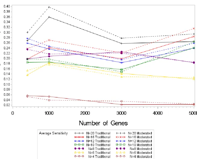
An analysis of the sensitivity values shows for larger samples of (n=16 and =20) there is a large increase in the sensitivity values. However as the number of samples decreases less of a difference is seen, with the traditional test statistic performing better at times or almost

equivalent. Note that the sensitivity values do not tend to increase as the number of genes increases, the sensitivity values decrease while the number of genes increase. Figure 4.1 shows that in disregard to the sample size, sensitivity values decrease as the number of genes increase. The sensitivity also increases along with the sample size; the sensitivity for a sample size of four is around 0.06 while the sensitivity for a sample size of 20 is around 0.30.

(33)

Figure 4.1. Average Sensitivity Values by Sample Size (4-20) by Test Statistic for Normal Simulations

(34)

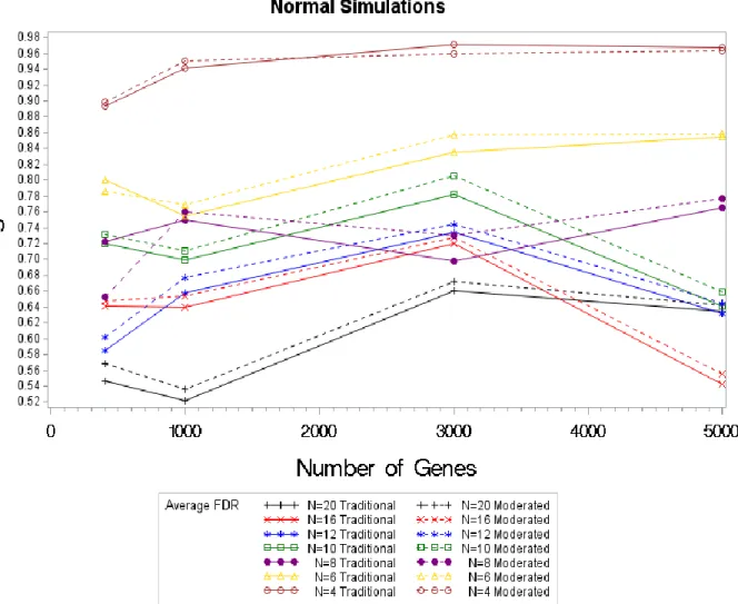
Comparison analysis of FDR and PPV will return the same result; FDR is complement of the PPV. If the moderated test statistic is superior to the traditional, it will have smaller false discovery rates, FDR. For the normal simulations, however an analysis of the FDR shows this is not the case. In the normal simulations the traditional test statistic had lower average FDRs, with the exception of the sample size of four and 3000 genes. A closer look at the simulation with a sample size of four shows that the FDRs for the moderated test statistic approaches the

traditional result. It is noteworthy that as the sample size increases the FDR decreases, showing that the DECODE method returned more correct classifications for HE/HC genes with a larger sample size. For the sensitivity results, we see an increase in sensitivity as the sample size increase, this result as follows in the FDR’s. The FDR’s decrease as the sample size increases, thus showing that the DECODE methods reliability increases as the number of samples increase with disregard to the test statistic.

(35)

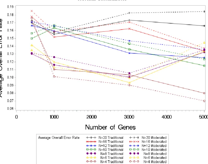
Figure 4.2. Average FDR Values by Sample Size (4-20) by Test Statistic for Normal Simulations For the sensitivity and the FDR, we were able to see a clear difference in the results for each sample size; however that is not the case for the overall error rates. Analysis of the overall error rates are difficult to interpret. There is a clear decrease in the overall error rate for a sample

(36)

Figure 4.3. Average Overall Error Rate Values by Sample Size (4-20) by Test Statistic for Normal Simulations

(37)

4.2.Breast Cancer Simulation Results

The Malaysian Breast Cancer study results were chosen to gain a better insight of how the DECODE methods would perform on real microarray data. The results of the normal

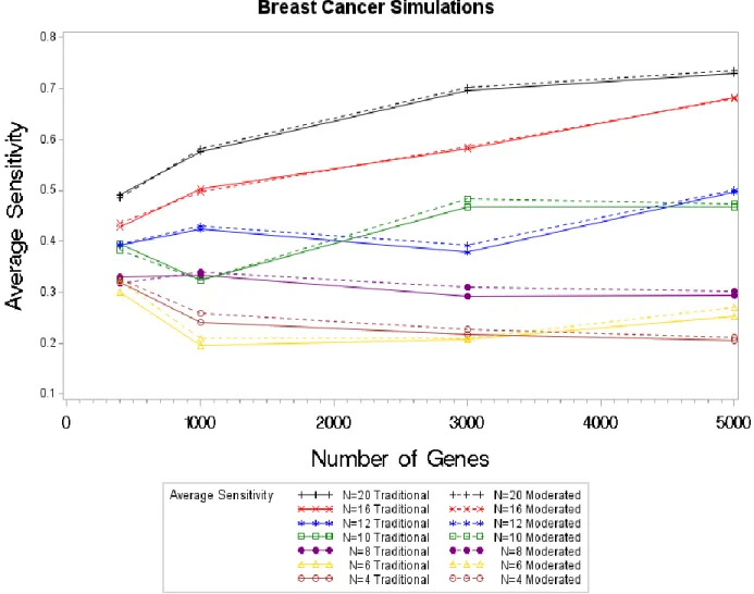
simulations showed a clear pattern of the sensitivity results for the moderated and traditional test statistic, however this pattern is not as apparent in the breast cancer sensitivity results. The sensitivity values are very similar for the moderated and the traditional test statistics. For the large sample sizes, there is a clear uptick in the sensitivity values for the moderated statistic, but not for a sample size of four or six. Our two smallest samples sizes returned almost equivalent sensitivity values. The sensitivity results for the moderated and the traditional test statistic are so close related for the breast cancer simulations that we are unable to say there is any real

difference between the results of the two test statistics.

Note that for the normal simulations, the sensitivity results started around 0.06 and increased as the sample size increased. For the breast cancer simulations, the sensitivity results start around 0.2 and increase as the sample size increases. Thusly, microarray simulations

returned slightly higher sensitivity values; this can be attributed to the presence of the underlying structures in microarray simulations.

(38)

Figure 4.4. Average Sensitivity Values by Sample Size by Test Statistic for Breast Cancer Simulations

(39)

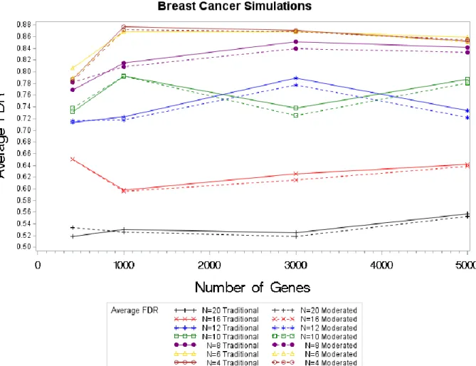
For the FDR, the results of the DECODE method using the moderated test statistic must exceed the traditional in order to be considered an improvement. For the two smallest sample sizes, the FDRs are similar between the two methods; a slight detectable decrease is noted for the moderated test statistic. We wouldn’t expect the moderated test statistic to outperform the

traditional test statistic in large samples to the same extent in the small sample sizes. However for the FDRs for the breast cancer simulation with n= 16 and n = 20 , the moderated returns slightly lower FDRs. This difference then extends to sample sizes of 8, 10 and 12 where a slightly larger decrease in noted for the moderated test statistic’s FDR. The larger sample sizes also return smaller FDR’s than that of the smaller samples. The FDR’s also decreased as the sample sizes increased; this same result was seen in our normal simulations.

(40)

(41)

4.3.Psoriatic Simulation Results

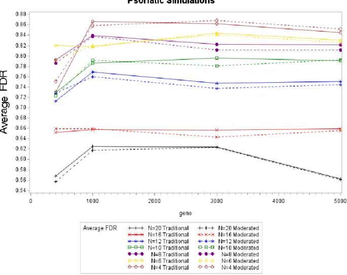
The Psoriatic simulations were performed with the goal of seeing whether the same results were seen as the Breast Cancer simulations. For the normal simulations and the breast cancer simulations, the FDR’s were closely related with the moderated surpassing the traditional at times. For the Psoriatic simulations the moderated test statistic is seen to perform better than the traditional except with a sample size of 20. For the small sample sizes (n=4 and n=6) only a slight difference in FDR is noted for the moderated test statistic with the traditional performing marginally better for a sample of 3000 genes and 5000 genes. This result is potentially due to the poor estimation of DC for the smaller sample sizes. This result shows evidence to support that hypothesis that the moderated test statistic is an improvement when used for smaller sample sizes with the exception of a sample size of four. All of simulations showed that as the sample size increases the FDR’s decrease, showing that when possible a larger sample size should be used in order to decrease the FDR’s.

(42)

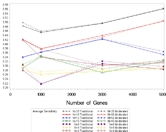
Figure 4.6. Average FDR Values by Sample Size by Test Statistic for Psoriatic Simulations In the psoriatic simulations the average sensitivity, the proportion of genes that truly are HE/HC and found to be HE/HC, varies for each sample size. The trend of decreasing sensitivity as the sample size decreases in not as noticeable for these results. The sensitivities for a sample size of four are larger than that for sample sizes of six and eight. In the two previous simulations, a decreasing sensitivity was seen as the sample size decreased. The results for sensitivity are different than expected however still showing that a large sensitivity is gained by using the moderated test statistic with the exception of n=16 where the sensitivity appears to be lower.

(43)

Figure 4.7. Average Sensitivity Values by Sample Size by Test Statistic for Psoriatic Simulations

In the normal simulations, the overall error rate increased as the sample size increased. However in the psoriatic simulations the overall error rate fell as the sample size increased. From Figure 4.8, it can be seen that the overall error rate was greatly decreased by the moderated test

(44)

Figure 4.8. Average Overall Error Rate Values by Sample Size by Test Statistic for Psoriatic Simulations

(45)

CHAPTER 5.CONCLUSION AND DISCUSSION 5.1.Conclusion

In this research, the moderated test statistic and the traditional test statistic were compared when implementing the DECODE method for gene expression analysis. The

hypothesis of this research was that using the moderated test statistic for estimating differential expression would be superior to using traditional test statistic for experiments with smaller sample sizes. In order to investigate this hypothesis, simulation studies were performed.

It was expected that there would be a sizable different in the sensitivity, PPV, FDR, and overall error rate for the moderated test statistic. However a lesser difference than expected was seen in the normal, breast cancer, and psoriatic simulations. A slight uptick in sensitivity was notice in all three simulations, with the most noticeable results seen in the breast cancer

simulations. As for the FDR results, the moderated test statistic returned smaller results for both microarray simulations studies but not for the normal simulation study. Since the moderated test statistic was seen as an improvement to the FDR results for both microarray simulations, we can assume that the result was not seen in the normal due to the missing underlying gene structure. In regards to the overall error rate, only slight differences were seen in the breast cancer

simulations, with more noticeable differences seen in the normal and psoriatic simulations. For the normal and psoriatic simulations there a noticeable decrease in the overall error rate for a

(46)

5.2.Recommendations

Even though the results were not as contrasting as expected, the moderated test statistic performed marginally better than the traditional test statistic in most cases when sample sizes were small. The one exception to this was with the smallest sample size, n=4, when the traditional statistic performed better. In my opinion, I would suggest using the moderated statistic in the DECODE method for all sample sizes. I make this suggestion even for large sample sizes considering the results were similar for the large sample sizes if not equivalent. Furthermore, the DECODE method returns smaller FDR and large sensitivity values for larger sample sizes. It would be recommendable to use a larger sample size when possible for the DECODE method.

5.3.Future Work

When considering Sensitivity, PPV, FDR, and overall error rate for all three simulations with a sample size of four, the results were similar for the moderated and traditional test

statistics. This result may be due to the sample size needed for calculation of the Z measure. In the methodology for the Z measure, it was noted that the smallest possible sample size was four. For future research, it would be advantageous to implement a different method of differential co-expression in order to apply this method to even smaller gene co-expression studies. A new method of differential co-expression maybe beneficial for sample sizes between 4 and 10, considering that de la Fuente A stated that more than 10 replicates is need for a reliable result (de la Fuente, 2010).

(47)

REFERENCES

Amar, D. S. (2013). Dissection of Regulatory Networks that are Altered in Disease via Differential Co-expression. PLoS Computational Biology, 9(3), e1002955.

Benjamini, Y. &. (1995). Controlling the false dicovery rate: a practical and powerful approach to multiple testing. Journal of the royal statistical society. Series B (Methodological), 289-300.

Bonferroni, C. (1936). Teoria statistica delle classi e calcolo delle probabilita. Pubblicazioni del R Instituto Superiore di Scienze Ecnonomiche e Commericiali di Firenze(8), 3-62. Cho, S. B. (2009). Identifying Set-Wise Differential Co-Expression in Gene Expression

Microarray Data. BMC Bioinformatics, 10(1), 109.

Choi, Y. K. (2009). Statistical Methods of Gene Set Co-Expression Analysis. Bioinformatics, 25(21), 2780-2786.

de la Fuente, A. (2010). From 'differetial expression' to 'differential networking' - identification of dysfunctional regulatory networks in disease. Trends in Genetics, 26(7), 326-333.

Gene Expression Omnibus (GSE13355). (2009, January 25). Retrieved from National Center for

Biotechnology Information:

https://www.ncbi.nlm.nih.gov/geo/query/acc.cgi?acc=GSE13355

Gene Expression Omnibus (GSE15852). (2009, April 28). Retrieved from National Center for

Biotechnology Information:

https://www.ncbi.nlm.nih.gov/geo/query/acc.cgi?acc=GSE15852

Gene Expression Omnibus. (2018). Retrieved from National Center for Biotechnology

Information: https://www.ncbi.nlm.nih.gov/geo/

Holm, S. (1979). A simple sequentially rejective multiple test procedure. Scandinavian journal of statistics, 65-70.

(48)

NI, I. P. (2010). Gene expression patterns distinguish breast carcinomas from normal breast tissues: the malaysian context. Pathology-Research and Practice, 206(4), 223-228. Roberto A., T. M. (2014). Loss of Connectivity in Cancer Co-Expression Networks. PLoS ONE,

9(1), e87075.

Smyth, G. K. (2004). Linear Models and Empirical Bayes Methods for assessing Differential Expression in Microarray Experiments. Statistical Applications in Genetics and Molecular Biology, 3(1), 1-25.

Storey, J. D. (2003). Statistical significane for genomewide studies. Proceedings of the National

Academy for Sciences, 100(16), 9440-9445.

Subramanian, A. T. (2005). Gene set enrichment analysis: A knowledge-based approach for interpreting genome-wide expression profiles. Proceedings of the National Academy of Sciences of the United States of America, 102(43), 15545-15550.

Troyanskaya, O. G. (2002). Nonparametric methods for indentidying differentially expressed genes in microarry data. Bioinformatics, 18(11), 1454-1461.

Tusher, V. G. (2001). Significance Analysis of Mircoarrays Applied to the Ionizing Radiation Response. Proceedings of the National Academy of Sciences of the United States of America, 98(9), 5116-5121.

Wang, D. W. (2017). BFDCA: A Comperhensive Tool of Using Bayes Factor for Differenital Co-Expression Analysis. Journal of Molecular Biology, 429(3), 446-453.

Watson, M. (2006). CoXpress: differential co-expression in gene expression data. BMC Bioinformatics, 7, 509.

William T. Barry, A. B. (2005). Significance analysis of functional categories in gene expression studies: a structured permutation approach. Bioinformatics, 21(9), 1943-1949.

(49)

APPENDIX. TABLES

Table A1

DECODE Method with Traditional Test Statistic (Normal Simulations with 400 genes)

Sensitivity PPV FDR Error Rate

Sample Average Standard Error Average Standard Error Average Standard Error Average Standard Error 100 0.5208 0.0574 0.6019 0.0665 0.3981 0.0665 0.1363 0.0159 80 0.4628 0.0550 0.5097 0.0661 0.4903 0.0661 0.1622 0.0166 60 0.4398 0.0570 0.5390 0.0655 0.4610 0.0655 0.1580 0.0155 40 0.4457 0.0514 0.5650 0.0631 0.4350 0.0631 0.1184 0.0220 20 0.2690 0.0402 0.4535 0.0639 0.5465 0.0639 0.1695 0.0186 16 0.1983 0.0291 0.3584 0.0620 0.6416 0.0620 0.1777 0.0141 12 0.2596 0.0347 0.4151 0.0593 0.5849 0.0593 0.1663 0.0205 10 0.1856 0.0264 0.2798 0.0521 0.7202 0.0521 0.1498 0.0115 8 0.1977 0.0329 0.2777 0.0537 0.7223 0.0537 0.1303 0.0203 6 0.1376 0.0260 0.1997 0.0424 0.8003 0.0424 0.1413 0.0150 4 0.0569 0.0159 0.1067 0.0356 0.8933 0.0356 0.1713 0.0234 Table A2

DECODE Method with Moderated Test Statistic (Normal Simulations with 400 genes)

Sample Average Standard Error Average Standard Error Average Standard Error Average Standard Error 100 0.5512 0.0592 0.5952 0.0659 0.4048 0.0659 0.1305 0.0164 80 0.5215 0.0560 0.5248 0.0649 0.4752 0.0649 0.1537 0.0173 60 0.4790 0.0583 0.5281 0.0642 0.4719 0.0642 0.1537 0.0160 40 0.4984 0.0549 0.5505 0.0616 0.4495 0.0616 0.1508 0.0173

(50)

Table A3

Sample Average Standard Error Average Standard Error Average Standard Error Average Standard Error 100 0.3746 0.0580 0.3633 0.0656 0.6367 0.0656 0.1794 0.0156 80 0.5758 0.0592 0.5843 0.0648 0.4157 0.0648 0.1293 0.0164 60 0.5189 0.0583 0.5547 0.0645 0.4453 0.0645 0.1420 0.0154 40 0.4485 0.0553 0.4914 0.0644 0.5086 0.0644 0.1564 0.0148 20 0.3986 0.0474 0.4634 0.0607 0.5366 0.0607 0.1578 0.0138 16 0.2708 0.0431 0.3457 0.0592 0.6543 0.0592 0.1588 0.0133 12 0.2469 0.0378 0.3233 0.0561 0.6767 0.0561 0.1658 0.0146 10 0.1969 0.0321 0.2894 0.0556 0.7106 0.0556 0.1668 0.0161 8 0.2171 0.0358 0.2400 0.0504 0.7600 0.0504 0.1260 0.0100 6 0.1780 0.0323 0.2308 0.0482 0.7692 0.0482 0.1133 0.0110 4 0.0396 0.0124 0.0491 0.0218 0.9509 0.0218 0.1013 0.0144

(51)

Table A5

Sample Average Standard Error Average Standard Error Average Standard Error Average Standard Error 100 0.4729 0.0612 0.5008 0.0682 0.4992 0.0682 0.1503 0.0165 80 0.4761 0.0605 0.4849 0.0662 0.5151 0.0662 0.1554 0.0160 60 0.4680 0.0604 0.4866 0.0644 0.5134 0.0644 0.1625 0.0175 40 0.5006 0.0570 0.5394 0.0629 0.4606 0.0629 0.1480 0.0161 20 0.2778 0.0466 0.3283 0.0588 0.6717 0.0588 0.1824 0.0169

(52)

Table A7

Sample Average Standard Error Average Standard Error Average Standard Error Average Standard Error 100 0.5046 0.1033 0.4754 0.1082 0.5246 0.1082 0.1451 0.0277 80 0.4513 0.0926 0.4692 0.1063 0.5308 0.1063 0.1621 0.0254 60 0.6133 0.0994 0.5812 0.0973 0.4188 0.0973 0.1251 0.0257 40 0.6459 0.0897 0.6167 0.0923 0.3833 0.0923 0.1082 0.0211 20 0.2948 0.0795 0.3581 0.0998 0.6419 0.0998 0.1843 0.0238 16 0.3161 0.0746 0.4440 0.1016 0.5560 0.1016 0.1373 0.0148 12 0.2591 0.0642 0.3549 0.0972 0.6451 0.0972 0.1359 0.0106 10 0.2646 0.0638 0.3406 0.0925 0.6594 0.0925 0.1235 0.0144 8 0.1852 0.0518 0.2228 0.0827 0.7772 0.0827 0.1352 0.0217 6 0.1273 0.0415 0.1409 0.0604 0.8591 0.0604 0.1446 0.0257 4 0.0252 0.0252 0.0362 0.0362 0.9638 0.0362 0.0699 0.0099

(53)

Table A9

DECODE Method with Traditional Test Statistic (Breast Cancer Simulations with 400 genes)

Sample Average Standard Error Average Standard Error Average Standard Error Average Standard Error 20 0.4904 0.0260 0.4811 0.0204 0.5189 0.0204 0.0601 0.0089 16 0.4279 0.0268 0.3499 0.0211 0.6501 0.0211 0.0844 0.0088 12 0.3931 0.0306 0.2870 0.0237 0.7130 0.0237 0.1298 0.0138 10 0.3937 0.0272 0.2684 0.0188 0.7316 0.0188 0.1058 0.0124 8 0.3300 0.0286 0.2315 0.0227 0.7685 0.0227 0.1690 0.0158 6 0.2997 0.0314 0.1935 0.0250 0.8065 0.0250 0.2103 0.0203 4 0.3197 0.0303 0.2128 0.0282 0.7872 0.0282 0.2434 0.0179 Table A10

DECODE Method with Moderated Test Statistic (Breast Cancer Simulations with 400 genes)

Sample Average Standard Error Average Standard Error Average Standard Error Average Standard Error 20 0.4854 0.0269 0.4667 0.0188 0.5333 0.0188 0.0599 0.0089 16 0.4355 0.0276 0.3498 0.0205 0.6502 0.0205 0.0867 0.0092 12 0.3947 0.0317 0.2835 0.0241 0.7165 0.0241 0.1276 0.0140 10 0.3837 0.0250 0.2620 0.0186 0.7380 0.0186 0.1089 0.0126 8 0.3181 0.0302 0.2180 0.0242 0.7820 0.0242 0.1681 0.0162 6 0.3221 0.0335 0.2107 0.0277 0.7893 0.0277 0.1989 0.0189 4 0.3265 0.0314 0.2156 0.0289 0.7844 0.0289 0.2397 0.0186

(54)

Table A11

(55)

Table A13

(56)

Table A15

(57)

Table A17

DECODE Method with Traditional Test Statistic (Psoriatic Simulations with 400 genes)

DECODE Method with Moderated Test Statistic (Psoriatic Simulations with 400 genes)

(58)

Table A19