University of Cape Town
Estimating Dynamic Affine Term Structure
Models
Zachry Pitsillis
A dissertation submitted to the Faculty of Commerce, University of Cape Town, in partial fulfilment of the requirements for the degree of Master of Philosophy.
February 12, 2015
M. Phil. in Mathematical Finance, University of Cape Town
The copyright of this thesis vests in the author. No
quotation from it or information derived from it is to be
published without full acknowledgement of the source.
The thesis is to be used for private study or
non-commercial research purposes only.
Published by the University of Cape Town (UCT) in terms
of the non-exclusive license granted to UCT by the author.
Declaration
I declare that this dissertation is my own, unaided work. It is being sub-mitted for the Degree of Master of Philosophy at the University of the Cape Town. It has not been submitted before for any degree or examination to any other University.
Zachry Pitsillis
Abstract
Duffee and Stanton (2012) demonstrated some pointed problems in estimat-ing affine term structure models when the price of risk is dynamic, that is, risk factor dependent. The risk neutral parameters are estimated with precision, while the price of risk parameters are not. For the Gaussian models they in-vestigated, these problems are replicated and are shown to stem from a lack of curvature in the log-likelihood function. This geometric issue for identifying the maximum of an essentially horizontal log-likelihood has statistical mean-ing. The Fisher information for the price of risk parameters is multiple orders of magnitude smaller than that of the risk neutral parameters. Prompted by the recent results of Christoffersen et al. (2014) a remedy to the lack of cur-vature is attempted. An unscented Kalman filter is used to estimate models where the observations are portfolios of FRAs, Swaps and Zero Coupon Bond Options. While the unscented Kalman filter performs admirably in identifying the unobserved risk factor processes, there is little improvement in the Fisher information.
Acknowledgements
I would like to express a deep thank you to my supervisors; doctor Peter Ouwehand and associate professor Thomas McWalter. Their guidance and in-sight has been invaluable. I am also deeply grateful for the warm and generous support from my parents. This dissertation could not have been completed without the love, friendship and direction which they provided.
Contents
1 Introduction 1
2 Affine Term Structure Models 3
2.1 Overview of the Affine Term Structure Literature . . . 3
2.2 Mathematical Framework for Term Structure Modelling . . . 6
2.3 Affine Term Structure Models . . . 8
2.4 Empirical Limitations of CATSMs . . . 10
2.5 Gaussian Models and a Dynamic Price of Risk . . . 11
3 Estimating Dynamic Affine Term Structure Models 14 3.1 Kalman Filtering and Gaussian DATSMs . . . 14
3.2 The Unscented Kalman Filter . . . 16
3.3 Maximum Likelihood Parameter Estimates . . . 21
4 Simulation Based Study of Parameter Estimates 23 4.1 Yields and the Kalman Filter . . . 23 4.2 FRAs, Swaps and Bond Options and the Unscented Kalman Filter . 29
5 Conclusion 33
Appendix A 34
Appendix B 35
List of Figures
1 Log-likelihoods at various parameter values using the Kalman filter and zero coupon bond yields. . . 27 2 Simulated and filtered states for the two factor model, using yields
and estimated parameters. . . 28 3 Simulated and filtered short rate using a portfolio of zero coupon bond
options and the unscented Kalman filter. . . 31 4 Log-likelihoods at various parameter values using the unscented Kalman
List of Tables
1 One factor Gaussian model parameter estimation results. . . 25 2 Two factor Gaussian model parameter estimation results. . . 25 3 Fisher information for the one factor Gaussian model estimated via
Kalman filter. . . 25 4 RMSE for the one and two factor models using true and estimated
parameters. . . 26 5 The portfolio of zero coupon bond options used to investigate the
performance of the unscented Kalman filter. . . 29 6 RMSE for the one factor models, using the true parameters with the
unscented Kalman filter and portfolios of non-linear instruments . . 29 7 Fisher information for the one factor Gaussian model estimated via
1
Introduction
Interest rate yield curves are inherently forward looking; they describe the costs of transferring cash-flows between parties through time. The term structure of interest rates thus has critical implications for future economic states. Piazzesi (2009) highlights the term structure’s importance for forecasting of interest rates, government debt policy, monetary policy and derivative and security pricing.
The modern economic treatment of term structures has centred on continuous time no arbitrage analysis of interest rates. Dai and Singleton (2003) view continuous time yield curve models in terms of three ingredients; the specification of risk neutral dynamics of risk factors, the dependence of interest rates on these risk factors and the associated risk factor premia. These three ingredients define a theoretical term structure model and are the key pieces to consider in connecting theoretical models to empirical observations.
Much of the econometric term structure modelling literature uses the affine class of models characterised by Duffie and Kan (1996). These models, termed completely affine, use a risk factor premium that is proportional to the volatility of the risk fac-tors and fixed in sign (typically negative). Empirical observations have forced affine models of the term structure to incorporate a more dynamic specification of their risk factor premia. In order to explain the joint behaviour of excess bond returns and bond yield volatility, the price of risk must be dynamic (state dependent). Suf-ficient theoretical flexibility, however, comes with challenges in estimating dynamic model parameters. These challenges were addressed by Duffee and Stanton (2012) for the recently developed dynamic term structure models. They investigated the capabilities of various methodologies for estimating models through a simulation based study.
The first aim of this dissertation is to follow in the footsteps of Duffee and Stan-ton (2012) in assessing methodologies for estimating dynamic affine term structure models. In particular, the efficacy of the Kalman filter when used to implement maximum likelihood parameter estimation will be investigated. Duffee and Stan-ton (2012) found that identification of parameters which characterise the dynamic price of risk is particularly problematic for Kalman filtering based estimation. These failings are expounded and analysed through simulation based studies.
It is found that the Fisher information for the parameters associated with the price of risk is orders of magnitude less than that of the other parameters. This has a natural geometric interpretation; the log-likelihood is effectively flat. Consequently, there is little precision in maximising the log-likelihood (estimating the parameters). The second aim of this dissertation is to investigate a potential innovation to the estimation of dynamic affine term structure models. It has recently been shown
by Christoffersen et al. (2014) that non-linear securities such as swaps and bond options can be used in an unscented Kalman Filter to effectively filter and forecast interest rates. Their investigation was conducted in a completely affine framework. They suggest that filters which incorporate enriched term structure information of-fer potential estimation improvements. This dissertation assess these potential im-provements for the estimation of dynamic affine term structure models. Despite the unscented Kalman filter providing quite remarkable accuracy for the identification of the state process, there is little improvement in the Fisher information.
In Chapter 2, the development of completely affine and then dynamic affine term structure models is reviewed. This is accompanied with an overview of the observations which force a dynamic price of risk and the subsequent estimation difficulties. Chapter 3 provides an exposition of the estimation procedures being investigated, while Chapter 4 contains the investigation methodology and results.
2
Affine Term Structure Models
2.1 Overview of the Affine Term Structure Literature
The empirical and theoretical investigation of interest rate term structures goes back to the work of Macaulay (1938), and there has since been a proliferation of literature on yield curves. Continuous time arbitrage free models of the yield curve were developed by Vasicek (1977) and Dothan (1978). Both authors relied on the specification of an underlying short rate diffusion. Combining the model of the instantaneous short rate with no arbitrage arguments, bond prices and hence a term structure can be derived. This approach was augmented with more unobserved state variables and generalised diffusion specifications, some notable examples of which are the work of Coxet al.(1985), Longstaff and Schwartz (1992) and Chen and Scott (1992). Many of the models were generalised and brought into a single consistent class of models by Duffie and Kan (1996). The class is referred to as affine term structure models, and has received much attention in the literature.
In the affine class of models bond yields are linear functions of the state variables. Duffee (2002) outlines that, depending on the form of the market price of interest rate risk, the linearity occurs in both the equivalent martingale measure and the physical measure. This relies on the market price of risk being proportional to the volatility of the risk factors, in which case the model is termed a completely affine term structure model (CATSM). This relationship is monotone; the market price of risk is only increasing or only decreasing with respect to the risk factor volatilities. The strict proportional characterisation of the market price of risk is, however, counter-factual. The observed means and volatilities of excess returns on longer dated bonds, driven by the market price of risk, is incompatible with the behaviour of yields in a completely affine framework. In particular, Duffee (2002) identified that CATSMs cannot simultaneously match the observed distribution of yields and capture the predictability of excess bond returns (from the slope of the yield curve). Consequently, Duffee (2002) finds that the forecast accuracy of CATSMs is poor due to these empirical mismatchings. Similar empirical failings of CATSMs were identified by Dai and Singleton (2002) and Duarte (2004).
Dai and Singleton (2003) emphasises that despite the particular failings the affine term structure models have provided much insight into the expectations hypothe-sis and term structures as a whole. Thus, it was not appropriate to discard the affine models, but rather, their limitations prompted the development of a second generation of models.
The second generation of affine term structure models include the classes of essentially affine models introduced by Duffee (2002) and the semi-affine class
intro-duced by Duarte (2004). Here, they are jointly termed dynamic affine term structure models (DATSMs). These models allow for a more general specification of the price of risk while remaining as tractable as the original affine models. Duffee (2002) modifies the price of risk in his essentially affine model so that strict dependence on the volatility of the factors is relaxed. The price of risk is allowed to vary with the level of the risk factors and it is also possible for it to change sign. These extensions facilitate term structures to be modelled in a more empirically consistent manner. Duarte (2004) used the same specification as Duffee (2002) for the market price of interest rate risk with an additional term, in essence allowing for even more volatility independent variation in the price of risk.
The additional flexibility in the specification of the price of risk in these dynamic affine models comes at the cost of parameter estimation. Duffee and Stanton (2012) show that the empirical literature assessing the performance of the second gener-ation affine models is sparse. In particular the finite sample behaviour of various estimation procedures requires attention. The asymptotic performance of maxi-mum likelihood estimators, efficient method of moment estimators and Kalman Fil-ter quasi-maximum likelihood is understood in general. However, the finite sample performance of these techniques when applied to second generation models requires further study.
Initial analysis of the use of Kalman filter in the context of first generation term structure models was undertaken by Duan and Simonato (1999) as well as by Lund (1995) and Lund (1997). The topic is still open with contemporary investigation of the use of the Kalman filter in completely affine term structure models undertaken by Christoffersenet al.(2014). Duffee and Stanton (2012) performed a Monte-Carlo study of the finite sample performance of various parameter estimation techniques for dynamic affine term structure models. Under various model specifications, with given parameters the state processes were simulated via a Milstein scheme and then different estimation techniques were applied. The input to the calibration techniques are bond yields, with or without added “observation” noise.
Duffee and Stanton (2012) find that for DATSMs some maximum likelihood parameters are estimated with little precision and are strongly biased. In addi-tion they find that when the likelihood is intractable the simulaaddi-tion based efficient method of moments does not yield usable parameter estimates while the Kalman filter was found to give parameter estimates which had similar finite sample biases to maximum likelihood. Note that the Kalman filter can be used to estimate both maximum likelihood models and models where exact maximum likelihood is not possible. When maximum likelihood is infeasible and the Kalman filter is used, the estimates obtained are quasi-maximum likelihood estimates.
The high levels of parameter estimate bias and standard deviation are endemic to the parameters which characterise the dynamic price of risk. In all of the DATSMs which Duffee and Stanton (2012) investigated the bias and standard deviation for these parameters far exceeded the bias and standard deviation for the risk neutral parameters. Recall that the combination of risk neutral parameters with the price of risk parameters determines the dynamics of the risk factor processes under the real world probability measure.
The bias and standard error associated with the risk neutral drift and volatility terms of the risk factor processes is small because these parameters are accessible through the entire term structure of bond yields at each observation. That is, risk neutral parameters are identified through the use of panel data and longitudinal data. Because of the dynamic specification of the price of risk only longitudinal information supports the estimation of the price of risk parameters. Duffee and Stanton (2012) state that, in a completely affine model, the risk neutral drift parameters “pin down” the drift of the risk factors in the real world, in essence, directing the price of risk parameter estimates. In the DATSMs the real world drift is decoupled from the risk neutral drift and hence the cross sectional information in term structure at each observation does not provide information for the price of risk parameters, only the time series evolution of the yields does so.
The lack of cross sectional information about the price of risk parameters in DATSMs motivates the need to enrich the longitudinal information available. In this regard Christoffersenet al.(2014) showed that non-linear security prices1(e.g. swaps and caps) can be used to effectively filter for the risk factors in completely affine term structure models (with known parameters). They investigate three types of filters incorporating non-linear dependence of the observed security prices on the risk factors; the extended Kalman Filter, the unscented Kalman filter and the particle filter. Each of these filters receives extensive exposition in the book by Haykin, et al. (2001). Motivation to use non-linear instruments as observations is given by the results of Almeidaet al. (2011), who find that using non-linear instruments greatly improves the forecasting of excess returns for swaps.
Christoffersenet al.(2014) find that the unscented Kalman filter provides accu-rate filtering of non-linear securities without the exorbitant computational burden of the particle filter. The extended Kalman filter was found to be inaccurate when the securities were highly non-linear functions of the state process. The accuracy which the unscented Kalman filter provides was found to facilitate effective param-eter estimation in the completely affine context. However, this was established via asymptotic argument rather than an entire Monte Carlo experimentation.
The success of Almeidaet al.(2011) in using instruments other than zero coupon bonds for the estimation of CATSMs naturally prompts the same inquiry into DATSMs. The further successes of Christoffersen et al. (2014) in the application of the unscented Kalman filter with non-linear instruments also encourages investi-gation. These results prompted the second step of this research to assess the viability of the unscented Kalman Filter for estimation of DATSMs. The driving question is whether the non-linearities in the risk factors for instruments such as FRAs, swaps and zero coupon bond options would resolve the lack of precision in the parameter estimates.
2.2 Mathematical Framework for Term Structure Modelling
This section is a brief exposition of term structure models based on the presenta-tion given by Piazzesi (2009). There are a number of important assumppresenta-tions which underlie the construction of a term structure model. In particular, the assumptions about risk preferences in the market as well as the absence of arbitrage and com-pleteness of a market dictate the framework in which bond yields are modelled. The fundamental building blocks of a term structure model is the risk free zero coupon bondPt(τ) with tenor τ =T −tand the instantaneous risk free short rate rt. The
yield to maturity, or yield, of a bond is the log return associated with holding the bond to maturity denoted by
y(tτ)=−logP (τ)
t
τ .
The short rate corresponds to the yield on an instantaneously maturing bond, that is
rt= limτ↓0y (τ)
t . Bond prices and the short rate can be related in any number of ways
based on the assumptions made about the market in which they are determined. A particularly general framework is that of martingale pricing theory. The details are suppressed here, suffice to say that if the market is arbitrage free and complete there exists a unique martingale probability measureQ, equivalent to the real-world (data generating or physical) probability measure P, under which bond prices are given by Pt(τ)=EQ exp − Z t+τ t rudu Ft
where Ft is the filtration generated by the relevant stochastic processes. In this
context we have used a money market account earning the short rate as a num´eraire which motivates callingQthe risk neutral measure. The details surrounding equiv-alent martingale pricing theory can be found in Bj¨ork (2004).
It is worth emphasising at this point that the observed yield curve at each date
through time for each tenor, τ, is determined by the real world measure P. So the cross sectional term structure is Q dependent and the longitudinal evolution is P dependent.
The sources of random variation which drive the evolution of bond prices (and hence the term structure of interest rates) are modelled asn risk factors,Xt∈Rn. These risk factors determine the short rate processrt=R(Xt) and are modelled as
It¯o processes with a stochastic differential equation
dXt=µ(t, Xt)dt+σ(t, Xt)dWft
underQ. HereWft is n-dimensional QBrownian motion, µ(t, Xt) is an n×1 vector
andσ(t, Xt) is andn×nmatrix. We write the correspondingPstochastic differential equation forXt as
dXt=ν(t, Xt)dt+σ(t, Xt)dWt
where Wt is n-dimensional P Brownian motion, µ(t, Xt) is an n×1 vector. The
technical restrictions onµ, ν and σ are suppressed for now.
The connection between P and Q is established in the specification of the one dimensional state price deflater process. Duffee (2002) gives that the state price deflater has the SDE
dπt=−rtπtdt−πtΛ(t, Xt)0dWt
where Λ(t, Xt) is an n×1 vector whose ith element represents the market price
of risk associated with the Brownian motion Wt(i). That is, the measure Q is the equivalent martingale measure given by Girsanov’s theorem such thatfWtwith SDE
dWft= dWt+ Λ(t, Xt)dt
is standard Brownian motion under Q. Consequently, the P dynamics of the risk factors can be written as
dXt= [µ(t, Xt) +σ(t, Xt)Λ(t, Xt)] dt+σ(t, Xt)dWt
The advantage of continuous time arbitrage free asset pricing is, as Piazzesi (2009) points out, that It¯o’s lemma facilitates the identification of arbitrage free prices from the specification of theQdynamics of the risk factors. The assumption that the risk factors are It¯o processes and hence Markovian implies we can rewrite the bond pricing equation as a direct function of the risk factorsXt, that is
Pt(τ)=F(t, τ, Xt).
Now if the functionF is sufficiently smooth, It¯o’s lemma can be used to establish a stochastic differential equation forPt(τ). Combining the resultant stochastic differen-tial equation with the known risk neutral drift ofPt(τ)allows for a partial differential equation for the bond price to be established, as follows.
The bond price has a QSDE given by
dF(t, τ, Xt) =µF(t, τ, Xt)dt+σF(t, τ, Xt)dfWt.
From It¯o’s lemma we can identify
µF(t, τ, Xt) =Ft(t, τ, Xt)+FX(t, τ, Xt)µ(t, Xt)+ 1 2tr σ(t, Xt)σ(t, Xt)0FXX(t, τ, Xt) ,
whereFt(t, τ, Xt) = ∂F(t,τ,X∂t t),FX(t, τ, Xt) is an 1×ngradient vector andFXX(t, τ, Xt)
is ann×nHessian matrix. In addition, we have that
σF(t, τ, Xt) =FX(t, τ, Xt)σ(t, Xt).
Now, the risk neutral dynamics ofF(t, τ, Xt) are known to follow
dF(t, τ, Xt) =rtF(t, τ, Xt)dt+σF(t, τ, Xt)dfWt
by the definition of the measureQ. Thus the bond price must satisfyrtF(t, τ, Xt) =
µF(t, τ, Xt), which gives the bond price partial differential equation
Ft(t, τ, Xt) +FX(t, τ, Xt)µ(t, Xt) + 1 2tr σ(t, Xt)σ(t, Xt)0FXX(t, τ, Xt) −rtF(t, τ, Xt) = 0.
2.3 Affine Term Structure Models
The affine class of models characterised by Duffie and Kan (1996) give a set of conditions on the risk factors, the short rate and the bond price function which are numerically tractable and have received much attention in the literature. The primary assumption of the affine class of models is that the bond price has an exponential-affine form F(t, τ, Xt) = exp A(τ)−B(τ)0Xt ,
where A and B are at least twice differentiable functions of τ. Duffie and Kan (1996) show that, under quite general technical conditions, the assumption of ex-ponentially affine bond prices implies thatµ(t, Xt),σ(t, Xt)σ(t, Xt)0 and rt are also
affine functions ofXt.
Following in the notation of Dai and Singleton (2000) we can write the parametri-sation for affine term structure models as follows. The short rate is given by
rt = δ0 +δ0XXt where δ0 is a real scalar and δX is an n×1 real vector. The
SDE ofXt is taken to be
dXt=eκ(θe−Xt)dt+ Σ p
whereκe and Σ aren×nmatrices,θeis ann×1 vector and Stis a diagonal matrix
with elements
[St]ii=αi+βi0Xt.
Under this parametrisation the bond prices can be identified through the solution of the coupled Ricatti equations
dA(τ) dτ =−θe 0 e κ0B(τ) +1 2 n X i=1 Σ0B(τ)2 i αi−δ0 and dB(τ) dτ =−eκ 0 B(τ)− 1 2 n X i=1 Σ0B(τ)2i βi+δX.
Here the notation [Σ0B(τ)]i indicates theith element of the vector Σ0B(τ), and the boundary conditions areB(0) = 0n×1 and A(0) = 0.
The completely affine term structure models are those in which theP dynamics of the risk factors are also required to be affine. That is the drift and the square of the diffusion are required to be affine functions of the risk factors. This imposes the assumption that the market price of risk is
Λt=
p
Stλ,
where λ is a n×1 real vector. The market price of risk relates only to the risk factors and does not depend on the maturity of any of the bonds in the market. This is an essential feature of all continuous time arbitrage free term structure models. In completely affine term structure models the market price of risk is strictly proportional to √St which drives the volatility of the risk factors. Note also that
the price of risk associated with each Brownian motion is either positive or negative. With this specification of the price of risk the PSDE of Xt is
dXt= h e κ(θe−Xt) + ΣStλ i dt+ ΣpStdWt dXt=κ(Θ−Xt)dt+ Σ p StdWt,
where κ = eκ−ΣΦ and Θ = κ−1(κeeθ+ Σψ), with the ith row of Φ given by λiβi0
andψ is ann×1 vector with elementsλiαi. From now on a completely affine term
structure model of this form will be referred to as a CATSM.
Naturally, there are a number of restrictions on the parameters which are required to ensure that the SDEs at hand have (strong) solutions. These restrictions, along with a classification scheme were developed by Dai and Singleton (2000). They call a modeladmissibleif its parameters ensure that [S(t)]ii is strictly positive for alli.
The primary characteristic of a CATSM is the number of factors, n. Then for
n-factor CATSMs Dai and Singleton (2000) show that there are n+ 1 are non-nested (distinct) subfamilies of admissible models each denoted byAm(n) withm=
0,1, . . . , n. The m here refers to the number of linearly independent combinations of risk factors which appear in the diffusion coefficient Σ√St. More specifically if we
setB= [β1, . . . , βn] thenm= rank(B). Essentially, each sub-family is characterised
by the total number of risk factors,n, and the number of these factors which affect the volatilities of the system,m.
Dai and Singleton (2000) define a canonical representation of the the subfamily
Am(n) as the least restrictiven-factor CATSM parametrisation which is admissible
and hasm= rank(B). There are technicalities about the uniqueness of the canonical representation given in the appendices of Dai and Singleton (2000). The subfamily Am(n) is precisely defined as the set of all CATSMs which are nested special cases
of the canonical representation for Am(n). One salient point to note is that the
processXtis stationary if the eigenvalues of κare are strictly positive. In addition,
Σ is restricted to be the identity matrix, essentially requiring each risk factor to represent a principle component of the term structure model. The specific parameter restrictions given by Dai and Singleton (2000) are listed in appendix A.
2.4 Empirical Limitations of CATSMs
There are a number of limitations associated with the completely affine interest rate models. Duffee (2002) reviews these limitations and summarises the mismatch between the empirical term structures and the models’. He highlights that affine models have poor forecast accuracy of expected excess returns on long dated bonds. This forecast inaccuracy stems from misspecification of the market price of interest rate risk. Problematically, the forecast errors in affine models are most pronounced when the yield curve is steeply upwards sloping. Non-zero correlations amongst the factors in combination with the price of risk specification implies unrealistic excess returns in long dated bonds. Furthermore, there is non-linear transformation in the term structure that the models fail to capture.
Duffee (2002) illustrates the impact of completely affine specification of the price of risk by considering the bond price SDE given by
dPt(τ) Pt(τ)
= (rt+e(tτ))dt+v
(τ)
t dWt.
In a completely affine context the excess return and volatility for a bond are
and
vt(τ)=−B(τ)0ΣpSt
respectively. Note the strict dependence on the risk factor volatility in both, and the consequent tight link between bond excess returns and bond return volatility.
Pronounced empirical mismatches relate to two of the stylised facts of term structures. Duarte (2004) summarises these stylised facts as i) “the excess return of treasury bonds has a high time variability” and ii) “the volatility of interest rates is time varying”. Affine term structure models in their initial form struggled to accommodate both these stylised facts due, in many cases, to the rigid specification of the market price of interest rate risk. In essence this is because their is a dynamic relationship between excess returns on treasury bonds and interest rate volatility. Dai and Singleton (2003) conclude that the empirical failings of affine term structure models are due to a “tension” within affine models between balancing the conditional expected returns and conditional volatilities with the fulcrum of the market price of interest rate risk. Specifically, the completely affine specification of the price of interest rate risk enforces a counter-factual proportional dependence of excess expected bond returns on risk factor volatilities.
2.5 Gaussian Models and a Dynamic Price of Risk
A second generation of affine term structure models was developed by Duarte (2004) and Duffee (2002), amongst others. Their innovation was to decouple the price of risk from the risk factor volatility. They both allow the price of risk to vary with the level of the risk factors. It was parameter estimates for the models developed by these authors which Duffee and Stanton (2012) investigated.
In order to keep the scope of this research manageable only the Gaussian models investigated by Duffee and Stanton (2012) are directly assessed here. The restriction of the investigation to only Gaussian models means that no approximations need to be made in both the simulation and estimation of the models. The Gaussian specification allows for affine yields and closed from bond option prices, in addition, the exact transition density for rt can be identified. These standard results are
presented in appendix B.
The focus on Gaussian models restricts the sources of error to the estimation procedures being investigated (as opposed to any approximations). In addition, it allows for computationally tractable extensions from the Kalman filter to the unscented filter. The existence of closed form pricing formulae for non-linear in-struments means that the unscented Kalman filter can be implemented without the need to invoke finite difference methods.
In the one factor Gaussian model the risk neutral dynamics of the short rate are
drt= (κθ−κrt)dt+σdfWt.
The two factor Gaussian model is given in Duffee and Stanton (2012) as
rt=δ0+X1t+X2t
dXit=−κiXitdt+σidWfit
fori= 1,2.
There are many alternative specifications of the price of risk in an affine modelling framework. The price of risk specification for Gaussian models which Duffee and Stanton (2012) investigate is given by
Λt=
λ1+λ2rt
σ
in the one factor case and by
Λit=
λi1+λi2Xit
σi
in the two factor case. These correspond to a special version of the price of risk supplied in Duffee (2002). Models with these specifications for the price of risk are termed here dynamic affine term structure models (DATSMs).
The key characteristic of these specifications is that the sign of the price of risk can change. This gives sufficient flexibility in the model to accommodate a dynamic relationship between volatility of bond returns (as well as risk factors) and the excess expected return. Duffee (2002) emphasises this flexibility. The interpretation is that DATSMs allow investors to seek and avoid different types of interest rate risk, this in turn facilitates (though does not guarantee) better empirical fit.
The added flexibility can be seen in the real world dynamics of the risk processes. In the one factor model the real world dynamics are
drt= ((κθ+λ1)−(κ−λ2)rt) dt+σdWt.
and in the two factor model
dXit= (λi1−(κi−λi2)Xit)dt+σidWfit.
The added flexibility in the price of risk decouples the risk neutral and real world drifts of the DATSM risk processes. This decoupling makes the identification of the price of risk parameters difficult, only longitudinal information can be used to identify the price of risk parameters. Cross-sectional information in the term structure only identifies the risk neutral parameters.
Through simulations Duffee and Stanton (2012) identify that the parameter esti-mates associated with the price of risk (λ1,λ2and the corresponding 2 factor param-eters) suffer from pronounced biases. In addition the standard deviations associated with these parameters were much larger than those associated with the risk neutral parameters. The characteristics of the parameters estimates were shared across the different estimation methods which Duffee and Stanton (2012) used. Both direct maximum likelihood and Kalman filtering (quasi or exact maximum likelihood) pro-duced biases and standard errors of the same magnitude. The efficient method of moments was found to produce much more severe biases and standard deviations.
3
Estimating Dynamic Affine Term Structure Models
3.1 Kalman Filtering and Gaussian DATSMs
The Kalman filter is a natural tool for the estimation of Gaussian affine term struc-ture models, enabled by the linear relationship between yields and risk factors. This presentation follows closely that of Duffee and Stanton (2012) with a little discussion. Consider the case of a known set of model parameters ρ. We observe a panel of
dzero-coupon bond yields as linear functions of them underlying risk factors with added observational noise
yt=H0(ρ) +H1(ρ)xt+t.
It is typical to assume that observation noise is addimensional serially independent Gaussian white noise with variance covariance matrixR(ρ). The observations noise is typically taken to represent market micro-structure noise, liquidity effects and other sources of variation not captured by the model.
For a chosen set of yield tenors{τ1, τ2, ..., τd} the observation matrices are given
by H0(ρ) = δ0−Pmi=1 Ai(τ1) τ1 .. . δ0−Pmi=1 Aiτ(τd) d , H1(ρ) = B1(τ1) τ1 . . . Bm(τ1) τ1 .. . B1(τd) τd . . . Bm(τd) τd .
Using Gaussian risk factors means that the unobserved state process evolves over discrete intervals in a linear fashion. In vector form
xt+1=F0(ρ) +F1(ρ)xt+vt+1
wherevt+1 is the innovations or news process driving the real world evolution of the risk factors. The innovations have variance covariance matrixQ(ρ). For the 2 factor case the vectorF0 and matricesF1 and Qhave values
F0(ρ) = κθi+λi1 κi−λi2 1−e−(κi−λi2)∆t i=1,2 F1(ρ) =diag h 1−e−(κi−λi2)∆t i i=1,2 Q(ρ) =diag σi2 2(κi−λi2) 1−e−2(κi−λi2)∆t i=1,2 .
In the one factor case, the above all become 1 dimensional and theisubscripts are dropped.
Note thatH0andH1depend on theQparameters and the cross-sectional tenors, while theF0, F1 and Qdepend on theP parameters and the observation time step ∆t.
For known parameters Haykin (2001)2 shows that the Kalman filter facilitates the minimum mean square error identification of the state variablext. The estimate
of the state is denotedxt|tand its covariance matrixPt|t. The Kalman filter requires
values for the unconditional mean and covariance of the state to start the process. These values can be calculated in the Gaussian case as
x0|0 =EP[xt] = κθi+λi1 κi−λi2 i=1...m P0|0 =V arP[xt] =diag σi2 2(κi−λi2) i=1...m .
At each time step with given estimates the step ahead forecasts of the statext+1|t
and its covariancePt+1|t are calculated from the state evolution equation by
xt+1|t=EP[xt+1|xt=xt|t] =F0(ρ) +F1(ρ)xt|t
and
Pt+1|t=V arP[xt+1|t|xt=xt|t] =F1(ρ)0Pt|tF1(ρ) +Q(ρ). This step ahead forecast facilitates a prediction of the observations
yt+1|t=EP[yt+1|xt=xt|t] =H0(ρ) +H1(ρ)xt+1|t
and the observation covariance
Vt+1|t=V arP[yt+1|xt=xt|t] =H1(ρ)0Pt+1|tH1(ρ) +R(ρ).
The prediction can be compared to the actual observation at t+ 1, which can then be used to improve the original state and covariance. The prediction error is given by
et+1=yt+1−yt+1|t,
which gives an updated estimator of the state and its covariance as
xt+1|t+1 =xt+1|t+Pt+1|tH1(ρ)Vt−+11|tet+1
Pt+1|t+1 =Pt+1|t−Pt+1|tH1(ρ)Vt−+11|tH1(ρ)
0
Pt+1|t.
The problem of finding the unknown true parametersρ◦ requires an appropriate objective function. This is supplied by the log-likelihood of the observations, which when maximised jointly minimises the observation prediction error and supplies maximum likelihood parameter estimates.
2The bookKalman Filters and Neural Networksis edited by Haykin and chapter 1 on Kalman
With the assumption of Gaussian measurement errors, the conditional density of the observationsf(yt|yt−1) is Gaussian with mean yt|t−1 and covariance matrix
Vt|t−1. The likelihood for a set of observationsy={y1, . . . yT}and for any parameter
vectorρ corresponds to a product of conditional densities
L(yt;ρ) = T
Y
t=1
f(yt|yt−1;ρ).
The parameters for a Gaussian DATSM model can thus be estimated by identifying the parameters which yield the maximum likelihood. This is achieved by finding the parameters which maximise the log-likelihood
`(ρ;y) =−1 2 T X t=1 h dlog(2π) + log|Vt|t−1|+e0tV −1 t|t−1et i ,
so that the parameter estimates are
ˆ
ρ(y) = max
ρ {`(ρ;y)}= maxρ {L(ρ;y)}.
The resulting optimisation problem of finding maximum likelihood parameter es-timates can be implemented with standard computation software available in pack-ages such asMatlab. However, a number of challenges exist when doing so. Gupta and Mehra (1974) describe the difficulties associated with finding the true maxi-mum likelihood. It is necessary to ensure that the starting point of the optimisation procedure are appropriate. In addition, it is necessary to conduct the optimisation multiple times using different starting points and algorithms in order to avoid ac-cepting a local maximum. It is also important to enforce the parameter restrictions implicit in the model.
The computational burden associated with the optimisation can become oner-ous. Analytical expressions for Jacobian (score) and Hessian matrices are possible, but difficult to establish with the models at hand. Consequently, computationally intensive derivative free optimisation needs to be employed. Even with analytical expressions of the derivatives numerical issues persist, remedies have been attempted such as square root filters implemented by Bierman et al. (1990) and later by Ku-likova (2009). These approaches may provide further numerical stability to the DATSM parameter estimation, but are not investigate here.
3.2 The Unscented Kalman Filter
The unscented Kalman filter was developed by Julier and Uhlmann (1997) for non-linear systems estimation and relies on the unscented transformation. This allows for
more accurate state estimation than if an extended Kalman filter3 were used. The key idea, as described by Wan and van der Merwe (2001), is to accurately capture the effect of non-linear transformations on means and variances with deterministic sampling points. This explanation follows that given by Wan and van der Merwe (2001) with simplifications to the application for the DATSMs at hand.
Firstly, it is necessary to understand the unscented transformation also devel-oped by Julier and Uhlmann (1996). The unscented transformation aims to closely approximate the mean and variance of non-linear transformation, G, of a vector random variable z with mean µz and covariance Σz. If the dimension of z is m
then 2m+ 1 vectors, called sigma vectors, are formed from points at scaled standard deviations away from the mean. The sigma vectorsZi are formed by
Z0 =µz Zi =µz+ ( p (m+ξ)Σz)i fori= 1. . . m Zi =µz−( p (m+ξ)Σz)i fori=m+ 1. . .2m.
where (p(m+ξ)Σz)i is the ith column of the Cholesky decomposition of (m+
ξ)Σz and ξ is a scaling parameter. In the Gaussian case the scaling parameter is
determined by ξ = 3α2−m, where α is set to a small positive number (typically less than 10−3). Each sigma vector is passed through the non-linear transformation to yield points
Gi=G(Zi), i= 0. . .2m,
which are used in a weighted average to estimate the mean and covariance
E[G(z)]≈ 2m X i=0 wi(1)Gi= ˆµg V ar[G(z)]≈ 2m X i=0 wi(2)(Gi−µˆg)(Gi−µˆg)0 = ˆΣg.
The mean weights are given by
w0(1)= ξ
m+ξ wi(1)= 1
2(m+ξ) i= 0. . .2m
3
The extended Kalman filter is much the same as the Kalman filter discussed in section 3.1, with the addition of first order Taylor series terms to the transition and observation equations to account for non-linearities. Most applications in which the state is non-Gaussian, i.e. a CIR process, use the extended Kalman Filter
and covariance weights w0(2)= ξ m+ξ + 3−α 2 wi(2)= 1 2(m+ξ) i= 0. . .2m.
The unscented Kalman filter follows the same steps as the Kalman filter with the use of the unscented transformation. Because of the use of Gaussian processes in the DATSM being investigated here a slightly simplified form of the unscented Kalman filter can be implemented. This corresponds to the unscented Kalman filter with additive noise as presented by Wan and van der Merwe (2001). We have that the process evolves linearly as before
xt+1=F0(ρ) +F1(ρ)xt+vt+1
where vt+1 is the innovations with variance covariance matrix Q(ρ). However, the observation are a non-linear function of the states
yt=H(xt;ρ)
that consists of a panel of security prices or rates. The panel of prices can include any number of securities from zero coupon bond yields to swap rates to bond option rates4
Again, consider the case of a known set of parameters ρ, we can initialise the state process as before at the unconditional mean and variance of the process
x0|0 =EP[xt]
P0|0 =V arP[xt]
Then for each time step of the observation t∈ {1. . . T} evolve the state and its covariance forward using the unscented transformation. This involves creating a set of sigma points5 Xt−1 = h xt−1|t−1, xt−1|t−1+γ q Pt−1|t−1, xt−1|t−1−γ q Pt−1|t−1 i
which are evolved through the state transition
Xt∗ =F(Xt−1;ρ)
4
Note one major advantage of this approach is that direct market observations can be used. For instance in the South African context coupon bearing bond yields (via the BESA formula) or FRA and swap rates including day count conventions
5
Hereγ=√m+ξandxt−1|t−1+γ p
Pt−1|t−1 means the matrix formed by the addition of each
column ofγp
where F(x) = F0(ρ) +F1(ρ)x. These evolved sigma points facilitate estimation of the state mean and covariance
xt|t−1= (2m) X i=0 wi(1)Xi,t∗ Pt|t−1= (2m) X i=0 wi(2)(Xi,t∗ −xt|t−1)(Xi,t∗ −xt|t−1)0+Q(ρ).
To forecast the observation it is first necessary to resample from the state process incorporating the forecast state covariance
Xt|t−1=hX0∗,t, X0∗,t+γqPt|t−1, X0∗,t−γ
q
Pt|t−1
i
.
These form estimates of the conditional observation mean and covariance
Yt|t−1 =H(Xt|t−1) yt|t−1 = (2m) X i=0 wi(1)Yi,t Vt|t−1 = (2m) X i=0 wi(2)(Yi,t−yt|t−1)(Yi,t−yt|t−1)0+R(ρ)
as well as the covariance between the observations and the state process
Jt|t−1 = (2m)
X
i=0
w(2)i (Xi,t−xt|t−1)(Yi,t−yt|t−1)0.
In the same manner as the Kalman filter the observation forecast error (yt−yt|t−1) is used to update the estimations of the state and its covariance
Kt=Jt|t−1Vt−|t−11
xt|t=xt|t−1+Kt(yt−yt|t−1)
Pt|t=Pt|t−1−KtVt|t−1Kt0.
In the case of unknown parameters it is, in general, not possible to identify the exact likelihood function. Because of the non-linear transformation the (in this application) Gaussian state process does not give a Gaussian observations. However, the unscented filter can be used to implement quasi-maximum likelihood, as the conditional mean and variance of the observations are accurately captured. So as with the Kalman filter an objective function can be formed from the (quasi) Gaussian log-likelihood. This assumption is typical in the literature, both Duffee and Stanton
(2012) and Christoffersenet al. (2014) use a Gaussian log-likelihood as an objective function.
The use of a quasi log-likelihood has been well established in the econometric literature. A deep presentation of this is give by White (1996). The core result is that in many cases the use of an appropriate quasi likelihood maintains consistency and lack of bias in the parameter estimates. With careful design the efficiency of the parameter estimates is only marginally comprised. Of course none of these favourable characteristic are always guaranteed in the limit, as in the case of the maximum likelihood parameters. It depends critically on the choice of the quasi likelihoods in relation to the true likelihood. And of course, the use of finite samples further obscures the behaviour of quasi maximum likelihood parameter estimates.
Christoffersenet al.(2014) use an approximate asymptotic argument to suggest the efficacy of the unscented Kalman filter with Gaussian quasi likelihood for pa-rameter estimation. They construct an approximation to the papa-rameter estimation error by first estimating the score statistics at the true parameters
ˆ
U(ρ◦i) = `(y;ρ
◦
i +ε)−`(y;ρ◦i −ε)
2ε i= 1. . . L
where ε is set to 10−6, L is the number of parameters and ρ◦ is the vector of
parameters. Then, using the likelihood Hessian matrix H(ρ◦) found using perfect filtering and second differencing, and they form an approximation to the parameter estimate error
ˆ
ρi−ρ◦i ≈Uˆ(ρ◦i)H−1(ρ◦)ii.
This is not strictly a measure of parameter error as Christoffersen et al.(2014) describe it. Most notably the scale of the values they report (in their Table 8) is vast compared to the actual parameters. Rather the quantity above, is a Hessian scaled score, and indicates the extent to which the log-likelihood has a maximum at the true parameter value, and thus the strength of the possibility that a maximum likelihood parameter estimate will be close to the true value. Their interpretation of the distribution of this error estimate is, however, appropriate. That the median Hessian scaled score is zero and that the unscented Kalman filter has a much smaller dispersion are good (though not conclusive) indicators of the efficacy of parameter estimation via the unscented Kalman filter. Zero valued scores are necessary for the parameter estimates to be close to the true values but not sufficient. The same complications discussed with maximising the log-likelihood supplied by the Kalman filter also apply to unscented Kalman filters.
3.3 Maximum Likelihood Parameter Estimates
A brief review of the theory of maximum likelihood parameter estimation is useful to illuminate some of the issues driving this investigation. Maximum likelihood estimators (MLEs) are central to the theory and practice of statistics. Their use is in many cases motivated by their limiting properties. An exposition of the theory of maximum likelihood and statistical inference are available in the book by Millar (2011).
The log-likelihood function is maximised by setting the scores
U(ρ) = ∂
∂ρ`(Y;ρ)
to zero. At the maximum likelihood parameters the scores are random variables with
EP[U(ρ◦)] = 0
The maximum likelihood parameters ˆρ(y) given in the case of the Kalman filter are random variables, dependent on the observations y. Provided the distribution of the sample satisfies some regularity conditions, MLEs have very favourable char-acteristics as the sample size tends to infinity. Firstly they are consistent, which is to say ˆρ(y) converges in probability to the true parameters ρ0. In addition, the limiting distribution is Gaussian,
√
T( ˆρ(y)−ρ0)
D
−→ N(0,I(ρ0)−1)
whereI(ρ0) is the Fisher information matrix associated with the parameters. This introduces the efficiency of MLEs, in the limit they achieve the Cramer-Rao lower bound on their covarianceI(ρ0)−1.
The Fisher information matrix is defined as
I(ρ0)ij =EP ∂ ∂ρi logf(Y;ρ) ∂ ∂ρj logf(Y;ρ) ρ=ρ0
which, under certain regularity conditions, becomes
I(ρ0)ij =−EP ∂2 ∂ρi∂ρj logf(Y;ρ) ρ=ρ0 .
The interpretation of the above quantity as information is seen through the ge-ometric notion of curvature. Barring some pathologies, the greater the (negative) curvature of the log density function around the true parameter the more informa-tion available for the parameter estimate. So when there is greater curvature in
the log-likelihood the the maximum of the likelihood can be identified with more precision. This feeds naturally into the statistical notion of variance, the greater the information the less variance there is, in the limit, for the MLE parameter estimate. The favourable performance of a maximum likelihood estimator for a finite sam-ple is not guaranteed from these characteristics. In fact it is the problems of finite sample MLEs that Duffee and Stanton (2012) investigate. Evaluation and analysis of the performance of MLEs is possible through comparison of the sample mean and variability of the estimators with their limiting distributional characteristics. Naturally, an assessment of the scores and Fisher information associated with each parameter then becomes useful.
4
Simulation Based Study of Parameter Estimates
The first step of this investigation is to replicate the results of Duffee and Stanton (2012) for one and two factor Gaussian models. The replication is largely successful, with very similar results being obtained. Then the significant parameter biases which Duffee and Stanton (2012) identified are explained through an analysis of the Fisher information for the parameters. It is found that the log-likelihood is essentially flat for the price of risk parameters. Consequently, the Fisher information for the price of risk parameters is comparatively tiny and hence they are estimated with little precision.In the second step an unscented Kalman filter is used to assess the viability of non-linear instruments for parameter estimation. Analysis of the quasi-log likeli-hood function is used to show that with moderately non-linear instruments (FRAs and Swaps) there is no improvement in the Fisher information. The use of zero coupon bond options provides a marginal improvement to the Fisher information. However, given the scale of the deficit of Fisher information, this improvement is not significant.
4.1 Yields and the Kalman Filter
The one and two factor Gaussian models described in section 2.5 were simulated using time steps of one week (∆t = 521) and T = 1000 observations. There were
n= 500 simulations conducted. The parameters used were the same as Duffee and Stanton (2012) (their Table 4) and are given here in Tables 1 and 2. From each simulation of the risk factors a set of of yields were then calculated on zero coupon bonds with tenors of 3 months, 6 months, 1 years, 5 years and 10 years. Then Gaussian noise, with standard deviation√V was added to the bond yields.
Each set of bond yields with noiseyk,k∈ {1, . . . , n}, was passed into an
optimi-sation routine which searches the parameter space for optimal parameters. At each parameter iteration the Kalman filter is called and the log-likelihood is identified, the optimisation iterates until a maximum for the log-likelihood is found. The op-timisation was conducted at least twice for each simulation, the opop-timisations are started with random parameters (in the space of possible parameters). In the event that the optimisation failed6 another set of starting parameters are generated. The constrained optimisation routines used were the Matlab routines active-set andsqp7.
6
Optimisation could fail for reasons including too many iterations, parameters on their boundary, failure of the Kalman filter for the given parameters and others
7
For details on these routines see http://www.mathworks.com/help/optim/ug/
To asses the performance of the parameter estimates Duffee and Stanton (2012) estimate the mean of the parameter estimates and their standard deviation. These quantities are compared to the true parameter and the estimated asymptotic stan-dard error of the parameter estimate. This asymptotic stanstan-dard error is calculated here using the inverse of the estimated Fisher information matrix. This is calculated by approximating the scores for each parameter and sample as a finite difference
ˆ
U(ρi;yk) =
`(yk;ρi+εi)−`(yk;ρi−εi)
2εi
i= 1. . . L, k= 1, . . . , n
whereεi = 20000ρi , the Fisher information is estimated by their covariance
ˆ
I(ρ)ij =cov( ˆU(ρi;y),Uˆ(ρj;y)).
The standard error is then
s.e(ρi) =
q
[ˆI(ρ)−1]
ii.
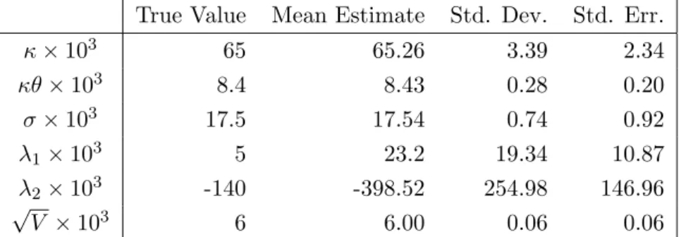
These estimates are shown in Tables 1 and 2. The estimates for the mean and standard deviation found in this study are close to those found by Duffee and Stanton (2012) (their Table 4). The standard error estimates found in this study are usually a bit lower than that of Duffee and Stanton (2012). The risk neutral parameters are estimated accurately, well within a standard deviation of their true values. The price of risk parameters, conversely, are estimated with little precision. There is substantial bias in the estimates and the standard deviation is an order of magnitude or two larger than that of the risk neutral parameters. The standard deviations of the risk neutral parameters are typically close to their lower bound8. For the price of risk parameters, the standard deviations were much larger than their asymptotic lower bounds. The impact of the bias in the price of risk parameters is econometrically significant. It leads to a misidentification of the expected excess bond return as well as an over estimation of the half life of economic shocks. These issues receive a full presentation in Duffee and Stanton (2012). The contribution of this research is rather to identify the cause of the parameter estimate inexactitude. The issue can be clearly seen in Figure 1 which shows the log likelihood func-tion at various parameter values for 20 samples of the one factor model. In each subplot the parameter in the x-axis is varied while the other parameters are kept at their true values. For the two risk neutral parameters plotted (κ and σ) the log likelihoods are concave and peaked close to the true parameter value. In such an environment the maximum is easy to identify (at least in one dimension). For
8
The standard deviations for σ and δ0 are actually below their lower bound estimate, this is probably due to the use of a finite difference calculation for the scores.
Table 1: One factor Gaussian model parameter estimation results. True Value Mean Estimate Std. Dev. Std. Err.
κ×103 65 65.26 3.39 2.34 κθ×103 8.4 8.43 0.28 0.20 σ×103 17.5 17.54 0.74 0.92 λ1×10³ 5 23.2 19.34 10.87 λ2×10³ -140 -398.52 254.98 146.96 √ V ×103 6 6.00 0.06 0.06 Table 2: Two factor Gaussian model parameter estimation results.
True Value Mean Estimate Std. Dev. Std. Err.
κ1×10³ 700 700.44 21.70 17.55 κ2×10³ 20 20.36 3.94 2.40 σ1×10³ 20 20.02 0.79 0.79 σ2×10³ 13 13.04 0.59 0.55 λ11×103 -10 -14.82 8.95 7.47 λ12×103 -4 -12.02 9.38 4.79 λ21×103 100 -133.41 292.61 122.11 λ22×103 -120 -412.42 222.84 183.34 δ0×103 100 100.20 5.39 5.61 √ V ×103 2 2.00 0.02 0.02
Table 3: Fisher information for the one factor Gaussian model estimated via Kalman filter.
Fisher Information Estimate ˆI(ρ◦)ii
κ 2385286 κθ 400917347 σ 4670803 λ1 64627 λ2 355 √ V 250647858
the price of risk parameters, however, the likelihood is essentially horizontal. It is not surprising therefore that the parameters are not identified with a great deal of precision. The initial visual evidence in Figure 1 is corroborated by the values in Table 3. The average curvature (Fisher information) of the likelihood in the price of risk parameters is substantially lower that that of the other parameters. Similar results were found in the in the two factor model.
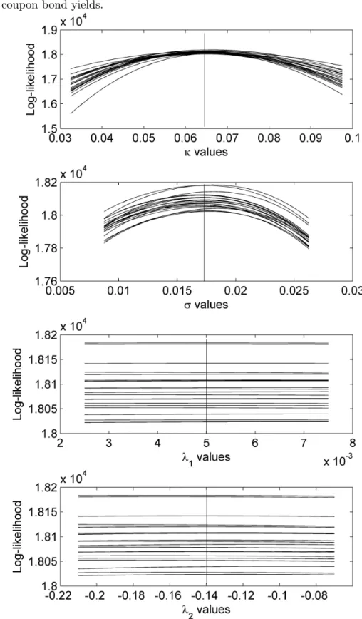
One final point to note about the Kalman filter implementation is its efficacy in identifying the states. Table 6 shows the Root Mean Square Error (RMSE) of the filtered state space when both the true parameters an estimated parameters are used. The scale of the risk factors in the simulation is in the order of 10−2, while the error is of the order 10−3. So the Kalman filter is accurately identifying the states when the true parameters are used. When the parameters are estimated the results are also good, with the two factor model providing slightly less accuracy. Figure 2 demonstrates these results for the simulated and filtered states for the two factor model, using estimated parameters.
Table 4: RMSE for the one and two factor models using true and estimated param-eters.
True Parameters Estimated Parameters One factor model 2.183×10⁻³ 2.184×10⁻³ Two factor model 1.833×10⁻³ 4.402×10⁻³ Note, for each path the parameter estimates found for that path are used.
Figure 1: Log-likelihoods at various parameter values using the Kalman filter and zero coupon bond yields.
Figure 2: Simulated and filtered states for the two factor model, using yields and estimated parameters.
4.2 FRAs, Swaps and Bond Options and the Unscented Kalman Filter
A one factor model is investigated using simulation and asymptotic arguments. The unscented filter is found to accurately filter for the state space process. However, there is only marginal improvement in the Fisher information for the price of risk parameters. It is found, however, that the use of options as observations improves the Fisher information for the volatility parameter.
Two investigations were undertaken. Both simulated the short rate from the one factor model, using the same true parameters as in table 1. The first investigation then calculated the rates for a 3m×6m FRA, 6m×1yr FRA, 2 year, 5 year and 10 year swap. The payment frequencies for the swaps are quarterly for the 2 year swap and half yearly for the 5 and 10 year swaps. The second investigation used a portfolio of zero coupon bond options, whose characteristics are given in Table 5. For the set of rates in the first investigation an observation error of√V = 0.006 was maintained, while for the options the observation error was set to√V = 0.6
Table 5: The portfolio of zero coupon bond options used to investigate the perfor-mance of the unscented Kalman filter.
Option Type Underyling Bond Maturity Option Maturity Strike (% of Underlying)
1 Call 2 Year 1 Year 98%
2 Put 2 Year 12 Year 110%
3 Call 5 Year 2 Year 110%
4 Put 5 Year 2 Year 130%
5 Put 10 Year 3 Year 130%
All options had a nominal of 100.
Table 6: RMSE for the one factor models, using the true parameters with the unscented Kalman filter and portfolios of non-linear instruments
RMSE with true parameters FRAs and Swaps 2.751×10⁻³
Bond Options 1.217×10⁻³
The unscented Kalman filter was found to be remarkably accurate at identifying the state process. The RMSE for both portfolios shown in Table 6. When zero coupon bond options are used the RMSE was just above 10 basis points, which is lower than when yields are used in the Kalman filter. This filtering efficacy is demonstrated in Figure 3. The RMSE for portfolio of FRAs and swaps was not as good, but still performed well at just under 30 basis points.
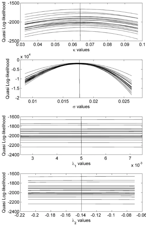
(quasi) Fisher information is calculated. A necessary, though not sufficient, condi-tion for the unscented Kalman filter to provide a solucondi-tion to the parameter estimate problem is for there to be a substantial improvement in the curvature of the quasi likelihood. Unfortunately, this is not provided. The Fisher information estimate for the original Kalman filter is given in Table 7 alongside the Fisher information obtained using the unscented Kalman filter for the two portfolios. There is no substantial improvement in the Fisher information when a portfolio of non-linear in-struments is used. It is encouraging, however, to see the substantial improvement in the Fisher information for the volatility parameter when zero coupon bond options are used. This is to be expected given the sensitivity of options to volatility parame-ters. Figure 4 shows the quasi log-likelihood for 20 samples using zero coupon bond options, demonstrating the improved curvature inσ and lack of curvature inλ1 and
λ2.
Table 7: Fisher information for the one factor Gaussian model estimated via the Kalman filter and unscented Kalman filter.
Fisher information for various filtering techniques ˆI(ρ◦)ii
Parameter KF with yields UKF with FRAs and Swaps UKF with ZCB options
κ 2385286 153325 308923 κθ 400917347 24266013 406251179 σ 4670803 1125481 275263064 λ1 64627 66055 71486 λ2 355 344 363 √ V 250647858 239824899 90648
The one factor Gaussian DATSM is the simplest possible model to assess the effi-cacy of parameter estimates. In the case of using yields as observations the Kalman filter provides exact maximum likelihood. The lack of curvature in the (quasi) Gaus-sian log-likelihood when various instruments are used is deeply problematic for the estimation of DATSMs. Any additional complexity such as the addition of factors or the use of square root processes requires further analytic and computational approx-imation. While these more complex models could be investigated, any meaningful improvement on the failures of the most basic case are extremely unlikely.
Figure 3: Simulated and filtered short rate using a portfolio of zero coupon bond options and the unscented Kalman filter.
Figure 4: Log-likelihoods at various parameter values using the unscented Kalman filter and zero coupon bond options.
5
Conclusion
Term structure modellers must sympathise with Yossarian9; observations have ne-cessitated the use of dynamic affine models, however observations are of little use for estimating the dynamic price of risk parameters. In the most basic Gaussian one factor model the price of risk parameters cannot be estimated with great precision with a reasonably sized sample. This effect is even more pronounced for the parame-ter which is introduced to make the price of risk state dependent. The lack of Fisher information for the price of risk parameters makes the log-likelihood effectively flat in these parameters. Consequently, any attempt to find a maximum is fated to be imprecise.
The root cause of the imprecision is identified by Duffee and Stanton (2012). When the price if risk is allowed vary, the drift of the real world risk factors is “decoupled” from the risk neutral parameters. More generally, a state dependent Radon-Nikodym derivative estranges the equivalent real world and risk neutral mea-sures. This constrains the statistical power and precision of parameter estimates. The rich information in the cross sectional observations, defined by the risk neutral measure, provides little guidance for the longitudinal processes, defined by the real world measure.
The difficulties induced by DATSMs are not, however, without value. They illustrate a key point for financial modelling. While many model classes may be able to recover stylised facts, the ability of the model to provide parameter estimates which are precise is, in many ways, more important. A sufficiently flexible model is of little use if the parameter estimates are too loose. In this regard, a simulation based analysis of the Fisher information for the model parameters before the use of data is vitally important.
9
Appendix A
The following definition of acanonical representation of the the subfamily Am(n) is
taken directly from Dai and Singleton (2000).
For eachm, we partition Xt as X= (XB, YD)0, whereXB ism×1 and XD is
(n−m)×1, and define the canonical representation ofAm(n) as the special case of
dXt=κ(Θ−Xt)dt+ Σ
p
StdWt,
with the following restrictions. Form >0 we have
κ= κBBm×m 0m×(N−m) κDB(n−m)×m κ(DDn−m)×(n−m)
and ifm= 0, κ must be upper or lower triangular. The other restrictions are
Θ = ΘBm×1 ΘD(n−m)×1 , Σ =In×n, α= 0m×1 1(n−m)×1 , B= Im×m Bm×(N−m) 0DB(n−m)×m 0(DDn−m)×(n−m) .
The corresponding restrictions on the parameters of the CATSM are
δXi≥0, m+ 1≤i≤n, κiΘ≡ m X j=1 κijΘj ≥0, 1≤i≤m, κij ≤0 1≤j ≤m, j6=i Θi ≥0, 1≤i≤m, Bm×(N−m) ≥0.
See Dai and Singleton (2000) for a discussion on why these restrictions ensure the admissibility of the model, and on the uniqueness of the representation.
Appendix B
These formulae are all based on the presentation given by Bolder (2001). The restrictions implicit in the DATSM model are that both σ and (κ−λ2) must be strictly positive. For ease of estimationκθ is treated as a single parameter.
In the one factor Gaussian model the risk neutral dynamics of the short rate are
drt= (κθ−κrt)dt+σdfWt
and with the price of risk specified as Λit = λ1+σλ2rt, the real world dynamics are
drt= ((κθ+λ1)−(κ−λ2)rt) dt+σdWt.
Then the affine yields for tenorτ are given by the standard Vasicek formulae
Y(τ) =−A(τ) τ + B(τ) τ rt where B(τ) = 1−e −κτ τ and A(τ) = κ 2θ−1 2σ 2 κ2 (B(τ)−τ)− σ2 4κB 2(τ).
Bond options with maturityT and strike K on a bond with tenor τ,Ptτ, are given by ct=PtτN(d1)−PtTKN(d2) pt=PtTKN(−d2)−PtτN(−d1) where d1 = log Pτ t KPT t +12σ2B σB d2 =d1− 1 2σB and σB2 =σ21−e −κ(τ−T) κ2 1−e−2κT 2κ .
Explicit formulae for the transition density are easily available with standard Ornstein-Uhlenbeck results. For given timest2 > t1 the distribution of rt2 given rt1
is Gaussian with EP[r t2|rt1] = κθ+λ1 κ−λ2 1−e−(κ−λ2)(t2−t1)+e−(κ−λ2)(t2−t1)rt1 and V arP[r t2|rt1] = σ2 2(κ−λ2) 1−e−2(κ−λ2)(t2−t1) .
References
Almeida, C., Graveline, J. J. and Joslin, S. (2011). Do interest rate options contain information about excess returns?,Journal of Econometrics164(1): 35 – 44. An-nals Issue on Forecasting.
URL:http://www.sciencedirect.com/science/article/pii/S0304407611000340
Bierman, G., Belzer, M., Vandergraft, J. and Porter, D. (1990). Maximum likeli-hood estimation using square root information filters, Automatic Control, IEEE Transactions on35(12): 1293–1298.
Bj¨ork, T. (2004). Arbitrage theory in continuous time, Oxford university press.
Bolder, D. (2001). Affine term-structure models: Theory and implementation, Work-ing Paper 01-15, Bank of Canada.
Chen, R.-R. and Scott, L. (1992). Pricing interest rate options in a two-factor Cox-Ingersoll-Ross model of the term structure,Review of Financial Studies5(4): 613– 636.
Christoffersen, P., Dorion, C., Jacobs, K. and Karoui, L. (2014). Nonlinear Kalman filtering in affine term structure models, Working Paper 14-04, Centre interuni-versitaire sur le risque, les politiques conomiques et l’emploi.
Cox, J. C., Ingersoll Jr, J. E. and Ross, S. A. (1985). A theory of the term structure of interest rates,Econometrica: Journal of the Econometric Societypp. 385–407.
Dai, Q. and Singleton, K. (2003). Term structure dynamics in theory and reality,
Review of Financial Studies16(3): 631–678.
Dai, Q. and Singleton, K. J. (2000). Specification analysis of affine term structure models, The Journal of Finance55(5): 1943–1978.
Dai, Q. and Singleton, K. J. (2002). Expectation puzzles, time-varying risk pre-mia, and affine models of the term structure, Journal of financial Economics
63(3): 415–441.
Dothan, L. U. (1978). On the term structure of interest rates,Journal of Financial Economics 6(1): 59–69.
Duan, J.-C. and Simonato, J.-G. (1999). Estimating and testing exponential-affine term structure models by Kalman filter,Review of Quantitative Finance and Ac-counting 13(2): 111–135.