Sensor-Based Reactive Navigation in Unknown Convex Sphere Worlds

University of Pennsylvania

ScholarlyCommons

Departmental Papers (ESE)

Department of Electrical & Systems Engineering

7-12-2016

Sensor-Based Reactive Navigation in Unknown

Convex Sphere Worlds

Omur Arslan

University of Pennsylvania, [email protected]

Daniel E. Koditschek

University of Pennsylvania, [email protected]

Follow this and additional works at:

https://repository.upenn.edu/ese_papers

Part of the

Electrical and Computer Engineering Commons, and the

Systems Engineering

Commons

Note: This paper was nominated for the Best Paper Award at the 12th International Workshop on the Algorithmic Foundations of Robotics in 2016. This paper is posted at ScholarlyCommons.https://repository.upenn.edu/ese_papers/840

For more information, please [email protected].

Recommended Citation

Sensor-Based Reactive Navigation in Unknown Convex Sphere Worlds

Abstract

We construct a sensor-based feedback law that provably solves the real-time collision-free robot navigation

problem in a compact convex Euclidean subset cluttered with unknown but sufficiently separated and strongly

convex obstacles. Our algorithm introduces a novel use of separating hyperplanes for identifying the robot’s

local obstacle-free convex neighborhood, affording a reactive (online-computed) piecewise smooth and

continuous closed-loop vector field whose smooth flow brings almost all configurations in the robot’s free

space to a designated goal location, with the guarantee of no collisions along the way. We further extend these

provable properties to practically motivated limited range sensing models.

Disciplines

Electrical and Computer Engineering | Engineering | Systems Engineering

Comments

Note: This paper was nominated for the Best Paper Award at the 12th International Workshop on the

Algorithmic Foundations of Robotics in 2016.

Sensor-Based Reactive Navigation

in Unknown Convex Sphere Worlds

Omur Arslan and Daniel E. Koditschek University of Pennsylvania, Philadelphia, PA 19103, USA

{omur,kod}@seas.upenn.edu

Abstract. We construct a sensor-based feedback law that provably solves the real-time collision-free robot navigation problem in a compact convex Euclidean subset cluttered with unknown but sufficiently separated and strongly convex obstacles. Our algorithm introduces a novel use of separating hyperplanes for identifying the robot’s local obstacle-free convex neighborhood, affording a reac-tive (online-computed) piecewise smooth and continuous closed-loop vector field whose smooth flow brings almost all configurations in the robot’s free space to a designated goal location, with the guarantee of no collisions along the way. We further extend these provable properties to practically motivated limited range sensing models.

Keywords: motion planning·collision avoidance·sensor-based planning

1

Introduction

Agile navigation in dense human crowds [1, 2], or in natural forests, such as now nego-tiated by rapid flying [3, 4] and legged [5, 6] robots, strongly motivates the development of sensor-based reactive motion planners. By the term reactive [7, 8] we mean that motion is generated by a vector field arising from some closed-loop feedback policy issuing online force or velocity commands in real time as a function of instantaneous robot state. By the termsensor-basedwe mean that information about the location of the environmental clutter to be avoided is limited to structure perceived within some local neighborhood of the robot’s instantaneous position — its sensor footprint.

In this paper, we propose a new reactive motion planner taking the form of a feedback law for a first-order (velocity-controlled), perfectly and relatively (to a fixed goal loca-tion) sensed and actuated disk robot, that can be computed using only information about the robot’s instantaneous position and structure within its sensor footprint. We assume the a priori unknown environment is a static topological sphere world [9], whose obsta-cles are convex and have smooth boundaries whose curvature is “reasonably” high rela-tive to their mutual separation. Under these assumptions, the proposed vector field plan-ner is guaranteed to bring all but a measure zero set of initial conditions to the desired goal. To the best of our knowledge, this is the first time a sensor-based reactive motion planner has been shown to be provably correct w.r.t. a general class of environments.

1.1 Motivation and Prior Literature on Vector Field Planners

The simple, computationally efficient artificial potential field approach to real-time ob-stacle avoidance [10] incurs topologically necessary critical points [11], which, in prac-tice, with no further remediation often include (topologically unnecessary) spurious

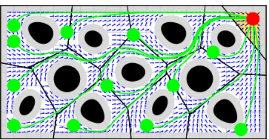
Fig. 1.Exact navigation of a disk-shaped robot using separating hyperplanes of the robot body (red at the goal) and convex obstacles (black solid shapes). Separating hyperplanes between the robot and obstacles define an obstacle-free convex neighborhood (the yellow region when the robot is at the goal) of the robot, and the continuous feedback motion towards the metric projec-tion of a given goal (red) onto this convex set asymptotically steers almost all robot configuraprojec-tions (green) to the goal without collisions along the way. The grey regions represent the augmented workspace boundary and obstacles, and the arrows show the direction of the resulting vector field. local minima. Even in topologically simple settings such as the sphere worlds ad-dressed here, constructions that eliminate these spurious attractors — e.g., navigation functions [12] — have largely come at the price of complete prior information.

Extensions to navigation functions partially overcoming the necessity of global prior knowledge of (and consequent parameter tuning for) a topologically and metri-cally simple environment have appeared in the last decade [13, 14]. Sequential compo-sition [15] has been used to cover complicated environments with cellular local potential decompositions [16], but still necessitating prior global knowledge of the environment.

1.2 Contributions and Organization of the Paper

This paper abandons the smooth potential field approach to reactive planning, achiev-ing an algorithm that is “doubly reactive” in the sense that not merely the integrated robot trajectory, but also its generating vector field can be constructed on the fly in real time using only local knowledge of the environment. Our piecewise smooth vector field combines some of the ideas of sensor-based exploration [17] with those of hybrid re-active control [16]. We use separating hyperplanes of convex bodies [18] to identify an obstacle-free convex neighborhood of a robot configuration, and build our safe robot navigation field by control action towards the metric projection of the designated point destination onto this convex set.

Our construction requires no parameter tuning and requires only local knowledge of the environment in the sense that the robot needs only locate those proximal obstacles determining its collision-free convex neighborhood. When the obstacles are sufficiently separated (Assumption 1 stipulates that the robot must be able to pass in between them) and sufficiently strongly convex at their “antipode” (Assumption 2 stipulates that they curve away from the enclosing sphere centered at the destination which just touches their boundary at the most distant point), the proposed vector field generates a smooth flow with a unique attractor at the specified goal along with (the topologically necessary number of) saddles — at least one associated with each obstacle. Since all of its critical points are nondegenerate, our vector field is guaranteed to steer almost all robot config-urations to the goal, while avoiding collisions along the way, as illustrated in Fig. 1.

It proves most convenient to develop the theoretical properties of this construc-tion under the assumpconstruc-tion that the robot can identify and locate those nearby obstacles whose associated separating hyperplanes define the robot’s obstacle-free convex neigh-borhood (a capability termed Voronoi-adjacent9_{obstacle sensing in Section 3.2), no}

matter how physically distant they may be. Thus, to accommodate more physically realistic sensors, we adapt the initial construction (and the proof) to the case of two different limited range sensing modalities, while extending the same formal guarantees as in the erstwhile (local but unbounded range) idealized sensor model.

In prior work [19], we propose a different construction based on power diagrams [20] for navigating among spherical obstacles using knowledge of Voronoi-adjacent9 obstacles to construct the robot’s local workspace [19, Eqn. (9)]. This paper introduces a new construction for that set in (7) based on separating hyperplanes, permitting an extension of the navigable obstacles to the broader class of convex bodies specified by Assumption 2, while providing the same guarantee of almost global asymptotic con-vergence (Theorem 3) to a given goal location. From the view of applications, the new appeal to separating hyperplanes permits the central advance of a purely reactive con-struction from limited range sensors (22), e.g., in the planar case from immediate line-of-sight appearance (27), with the same global guarantees.

This paper is organized as follows. Section 2 continues with a formal statement of the problem at hand. Section 3 briefly summarizes a separating hyperplane theorem of convex bodies, and introduces its use for identifying collision-free robot configurations. Section 4, comprising the central contribution of the paper, constructs and analyzes the reactive vector field planner for safe robot navigation in a convex sphere world, and provides its more practical extensions. Section 5 illustrates the qualitative properties of the proposed vector field planner using numerical simulations. Section 6 concludes with a summary of our contributions and a brief discussion of future work.

2

Problem Formulation

Consider a disk-shaped robot, of radiusr ∈ R>0 centered at x ∈ W, operating in a closed compact convex environmentW _{in the}n-dimensional Euclidean spaceRn, wheren≥2, punctured withm∈ Nopen convex setsO_{: ={}O1, O2, . . . , Om}with

twice differentiable boundaries, representing obstacles.1Hence, the free spaceF_{of the} robot is given by F_{: =}!_x∈W " " "B(x, r)⊆W\ #m i=1Oi $ , (1)

whereB(x, r) : =%q∈Rn""∥q−x∥< r&is the open ball centered atxwith radiusr, andB(x, r)denotes its closure, and∥.∥denotes the standard Euclidean norm.

To maintain the local convexity of obstacle boundaries in the free spaceF_{, we} as-sume that our disk-shaped robot can freely fit in between (and thus freely circumnavi-gate) any of the obstacles throughout the workspaceW_:2

1

Here,Nis the set of all natural numbers;RandR>0(R≥0) denote the set of real and positive (nonnegative) real numbers, respectively.

Assumption 1. Obstacles are separated from each other by clearance of at least

d(Oi, Oj) > 2r for alli ̸= j, and from the boundary∂Wof the workspaceW as

d(Oi,∂W_)>2rfor alli= 1. . . m, whered(A, B) : = inf%∥a−b∥""a∈A,b∈B&.

Before formally stating our navigation problem, it is useful to recall a known topo-logical limitation of reactive planners: if a continuous vector field planner on a gener-alized sphere world has a unique attractor, then it must have at least as many saddles as obstacles [9]. In consequence, the robot navigation problem that we seek to solve is:

Reactive Navigation Problem. Assuming the first-order (completely actuated single-integrator) robot dynamics,

˙x = u(x), (2)

find a Lipschitz continuous vector field controller,u :F_→Rn, that leaves the robot’s free spaceFpositively invariant and asymptotically steers almost all robot configura-tions inFto any given goal locationx∗_∈F.

3

Encoding Collisions via Separating Hyperplanes

3.1 Separating Hyperplane Theorem

A fundamental theorem of convex sets states that any two nonintersecting convex sets can be separated by a hyperplane such that they lie on opposite sides of this hyperplane:

Theorem 1 ([18, 21]).For any two disjoint convex setsA, B ∈Rn_{(i.e.,A∩B=∅),}

there existsa∈Rn_{andb∈Rsuch thata}T_{x≥bfor allx∈Aanda}T_{x≤bfor allx∈B.} For example, a usual choice of such a hyperplane is [18]:

Definition 1. Themaximum margin separating hyperplaneof any two disjoint convex setsA, B⊂Rn_{, withd(A, B)>0, is defined to be}

H(A, B) : =!x∈Rn " " "∥x−a∥=∥x−b∥,∥a−b∥=d(A, B),a∈A,b∈B $ , (3)

whered(x, H(A, B))≥ d(A,B₂ )for allx∈A∪B.

Another useful tool for finding separating hyperplanes is metric projection:

Theorem 2 ([21]).LetA⊂Rnbe a closed convex set andx∈Rn. Then there exists a unique pointa∗_{∈Asuch that}

a∗=ΠA(x) : = arg min a∈A

∥a−x∥, (4)

and one has(x−ΠA(x))T(ΠA(x)−a)≥0for alla∈A. The mapΠA(x)is called themetric projectionofxonto setA.

Lemma 1. The maximum margin separating hyperplane of a convex setA ⊂Rnand the ballB(x, r)of radiusr∈R>0centered atx∈Rn, satisfyingd(x, A)≥r, is given by

H(A, B(x, r)) =!y∈Rn " " " ' ' 'y−(ΠB(x,r)◦ΠA)(x) ' ' '=∥y−ΠA(x)∥ $ , (5) where(Π_B(x,r)◦Π_A)(x) = x−r x−ΠA(x) ∥x−ΠA(x)∥ .

Proof. See Appendix I-A in Supplementary Material. ! A common application of separating hyperplanes of a set of convex bodies is to dis-cover their organizational structure. For instance, to model its topological structure, we define the generalized Voronoi diagramsV _{={V1, V2, . . . , Vm} of a convex} environ-mentW_inRn_{populated with disjoint convex obstaclesO={O}

1, O2, . . . , Om}(i.e., d(Oi, Oj)>0for alli̸=j), based on maximum margin separating hyperplanes, to be3 4 Vi: =!q∈W""_{"∥q−pi∥ ≤ ∥q−pj∥,∥pi−pj∥=d(Oi, Oj),pi∈Oi,pj∈Oj ∀j̸=i}$_,(6) which yields a convex cell decomposition of a subset ofW_{such that, by construction,} each obstacle is contained in its Voronoi cell, i.e.,Oi ⊂ Vi, see Fig. 2. Note that for point obstacles, sayOi={pi}for somepi ∈ Rn, the generalized Voronoi diagram of

W_{in (6) simplifies back to the standard Voronoi diagram of}W_{, generated by points} {p1, . . . ,pm}, i.e.,Vi=

%

q∈W""∥q−pi∥ ≤ ∥q−pj∥, ∀j̸=i

& [27].

3.2 The Safe Neighborhood of a Disk-Shaped Robot

Throughout the sequel, we consider a disk-shaped robot, centered atx∈W_{with radius}

r ∈ R>0, moving in a closed compact convex environmentW⊆ Rn populated with open convex obstacles, O _{= {O1, O2, . . . , Om}, satisfying Assumption 1. Since the} workspace, obstacles, and the robot radius are fixed, we suppress all mention of the associated terms wherever convenient, in order to simplify the notation.

Using the robot body and obstacles as generators of a generalized Voronoi diagram ofW_{, we define the robot’s}local workspace,LW_{(x), illustrated in Fig. 2(left), as,}5

LW_{(x) : =} ( q∈W " " " " ' ' ' 'q−x +r x−Π_Oi(x) ! ! !x−ΠOi(x) ! ! ! ' ' ' '≤ ' 'q−Π_Oi(x)'', ∀i ) . (7) Note that we here take the advantage of having a disk-shaped robot and construct the maximum margin separating hyperplane between the robot and each obstacle using the robot’s centroid (Lemma 1).

A critical property of the local workspaceLW_is:

Proposition 1. A robot placementx∈W_\*m

i=1Oiis collision free, i.e.,x∈F, if and

only if the robot body is contained in its local workspaceLW_{(x), i.e.,}6

x∈F_{⇐⇒B(x, r)⊆}LW_{(x). (8)}

Proof. See Supplementary Material Appendix I-B. ! 3_{Generalized Voronoi diagrams and cell decomposition methods are traditionally encountered} in the design of roadmap methods [8,17,22]. A major distinction between our construction and these roadmap algorithms is that the latter typically seek a global, one-dimensional graphical representation of a robot’s environment (independent of any specific configuration), whereas our approach uses the local open interior cells of the robot-centric Voronoi diagram to deter-mine a locally safe neighborhood of a given free configuration.

4_{It seems worth noting that our use of generalized Voronoi diagrams is motivated by application} of Voronoi diagrams in robotics for coverage control of distributed sensor networks [23–26]. 5

Here, to solve the indeterminacy, we set _∥x_x∥ = 0wheneverx = 0. 6_{Note thatF"W\}!m

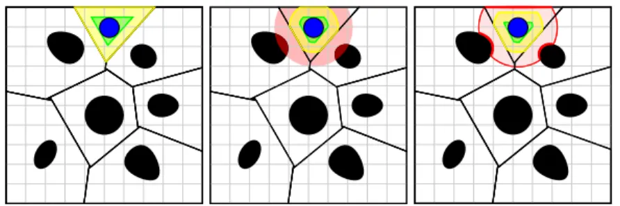
Fig. 2.Local workspaceLW_{(yellow) and local free space}LF _{(green) of a disk-shaped robot}

(blue) for different sensing modalities: (left) Voronoi-adjacent9obstacle sensing, (middle) a fixed radius sensory footprint (red), (right) a limited range line-of-sight sensor (red). The boundary of each generalized Voronoi cell is defined by the maximum margin separating hyperplanes of the robot body (blue) and obstacles (black).

Accordingly, we define the robot’slocal free space,LF_{(x), by eroding}LW_(x), removing the volume swept along its boundary,∂LW_{(x), by the robot body radius,} illustrated on the left in Fig. 2, as [28]7

LF_{(x) : =}LW_(x)\+_∂LW_(x)⊕B(0, r),=!q∈LW_(x) " " "B(q, r)⊆LW(x) $ . (9) Note that, for anyx∈F_,LF_{(x)is a nonempty closed convex set, becausex∈}LF_(x) and the erosion of a closed convex set by an open ball is a closed convex set.8

An immediate consequence of Proposition 1 is:

Corollary 1. Any robot placement in the local free spaceLF_(x) of a collision free robot locationx∈Fis also collision free, i.e.,LF_(x)⊆Ffor allx∈F.

Finally, it is useful to emphasize that to construct its local workspace, the robot re-quires only local knowledge of the environment in the sense that the robot only needs to locate proximal obstacles — those whose Voronoi cells are adjacent9_{to the robot’s}

(local workspace). This can be achieved by assuming an adjustable radius sensory foot-print and gradually increasing its sensing range until the set of obstacles in the sensing range satisfies a certain geometric criterion guaranteeing that the detected obstacles ex-actly define the robot’s local workspace [23]. We will refer to this sensing model as

Voronoi-adjacent obstacle sensing.

4

Robot Navigation via Separating Hyperplanes

In this section, first assuming Voronoi-adjacent obstacle sensing, we introduce a new provably correct vector field controller for safe robot navigation in a convex sphere world, and list its important qualitative properties. Then we present its extensions for two more realistic sensor models (illustrated, respectively, in the middle and the right panels of Fig. 2): a fixed radius sensory footprint and a limited range line-of-sight sensor.

7

Here,0is a vector of all zeros with the appropriate size, andA⊕Bdenotes the Minkowski sum of setsAandBdefined asA⊕B={a+b|a∈A, b∈B}.

8_{The erosion of a closed half-space by an open ball is a closed half-space, and a closed convex} set can be defined as (possibly infinite) intersection of closed half-spaces [18]. Thus, since the erosion operation is distributed over set intersection [28], and an arbitrary intersection of closed sets is closed [29], the erosion of a closed convex set by an open ball is a closed convex set. 9 _{A pair of Voronoi cells inR}n

4.1 Feedback Robot Motion Planner

Assuming the fully-actuated single-integrator robot dynamics in (2), for a choice of a desired goal locationx∗_{∈F, we propose a robot navigation strategy, called the “}

move-to-projected-goal” law,u :F_→Rn_{that steers the robot at locationx∈Ftowards the}

global goalx∗through the “projected goal”,ΠLF(x)(x∗), as follows:10 u(x) =−k+x−ΠLF(x)(x∗)

,

, (10)

wherek∈R>0is a fixed control gain andΠA(4) is the metric projection onto a closed convex setA ⊂ Rn, andLF_{(x)is continuously updated using the Voronoi-adjacent} obstacle sensing and its relation withLW_{(x)in (9).}

4.2 Qualitative Properties

Proposition 2. The “move-to-projected-goal” law in (10) is piecewise continuously differentiable.

Proof. An important property of generalized Voronoi diagrams in (6) inherited from the standard Voronoi diagrams of point generators is that the boundary of each Voronoi cell is a piecewise continuously differentiable function of generator locations [31, 32]. In particular, for anyx∈F_{, the boundary of the robot’s local workspace}LW_(x)is piece-wise continuously differentiable since it is defined by the boundary of the workspace and separating hyperplanes between the robot and obstacles, parametrized by xand

Π_Oi(x), and metric projections onto convex cells are piecewise continuously differ-entiable [33]. Hence, the boundary of the local free space LF_{(x) is also piecewise} continuously differentiable, because LF_{(x) is the nonempty erosion of} LW_{(x) by a} fixed open ball. Therefore, one can conclude using the sensitivity analysis of metric projections onto moving convex sets [34, 35] that the “move-to-projected-goal” law is Lipschitz continuous and piecewise continuously differentiable. !

Proposition 3. The robot’s free spaceF_{in (1) is positively invariant under the}

“move-to-projected” law (10).

Proof. SincexandΠLF(x)(x∗)are both inLF(x)for anyx∈F, andLF(x)is an ob-stacle free convex neighborhood of x (Corollary 1), the line segment joining xand

ΠLF(x)(x∗) is free of collisions. Hence, at the boundary of F, the robot under the “move-to-projected-goal” law either stays on the boundary or moves towards the in-terior ofF_{, but never crosses the boundary, and so the result follows. !}

Proposition 4. For any initial x ∈ F, the “move-to-projected-goal” law (10) has a unique continuously differentiable flow inF(1) defined for all future time.

10_{In general, the metric projection of a point onto a convex set can be efficiently computed using} an off-the-shelf convex programming solver [18]. IfWis a convex polytope, then the robot’s local free spaceLF_(x)is also a convex polytope and can be written as a finite intersection of half-spaces. Thus, the metric projection onto a convex polytope can be recast as quadratic programming and can be solved in polynomial time [30]. In the case of a convex polygo-nal environment,LF_{(x)is a convex polygon and the metric projection onto it can be solved}

Proof. The existence, uniqueness and continuous differentiability of its flow follow from the Lipschitz continuity of the “move-to-projected-goal” law in its compact do-mainF_{, because a piecewise continuously differentiable function is locally Lipschitz on} its domain [36], and a locally Lipschitz function on a compact set is globally Lipschitz

on that set [37]. !

Proposition 5. The set of stationary points of the “move-to-projected-goal” law (10) is{x∗_}∪*m i=1Si, where S_{i: =} ( x∈F " " " "d(x, Oi) =r, (x−Π_Oi(x))T(x−x∗₎ ∥x−Π_Oi(x)∥∥x−x∗_∥ = 1 ) . (11)

Proof. It follows from (4) andx∗_∈LF(x∗_{)that the goalx}∗_{is a stationary point of (10).}

In fact, for anyx∈F_{, one hasΠLF(x)(x}∗_{) = x}∗ _wheneverx∗_∈LF_{(x). Hence, in the} sequel of the proof, we only consider the set of robot locations satisfyingx∗_̸∈LF(x).

Letx∈F_{such thatx}∗_̸∈LF_{(x). Recall from (7) and (9) that}LW_{(x)is determined} by the maximum margin separating hyperplanes of the robot body and obstacles, and LF_{(x)is obtained by eroding}LW_{(x)by an open ball of radius}r. Hence,xlies in the interior ofLF_{(x)if and only if}d(x, Oi)> rfor alli. As a result, sincex∗ ̸∈LF(x),

one hasx =ΠLF(x)(x∗)only ifd(x, Oi) =rfor somei.

Note that ifd(x, Oi) =r, then, sinced(Oi, Oj)>2r(Assumption 1),d(x, Oj)> r for all j ̸= i. Therefore, there can be only one obstacle index i such that x =

ΠLW(x)(x∗)andd(x, Oi) = r. Further, givend(x, Oi) = r, sinceΠLF(x)(x∗)is the unique closest point of the closed convex setLF_{(x)to the goalx}∗_{(Theorem 2), its}

op-timality [18] implies that one hasx =ΠLW(x)(x∗)if and only if the maximum margin separating hyperplane between the robot and obstacleOiis tangent to the level curve of

the squared Euclidean distance to the goal,∥x−x∗_∥2_{, atΠ}

Oi(x), and separatesxand

x∗_{, i.e.,}

(x−ΠOi(x))

T_(x−x∗₎

∥x−ΠOi(x)∥∥x−x

∗_∥ = 1. (12)

Thus, one can locate the stationary points of the “move-to-projected-goal” law in (10) associated with obstacleOias in (11), and so the result follows. ! Note that, for any equilibrium pointsi ∈ Si associated with obstacleOi, one has

that the equilibriumsi, its projectionΠOi(si)and the goalx

∗_{are all collinear.}

Lemma 2. The “move-to-projected-goal” law (10) in a small neighborhood of the goal

x∗_{is given by}

u(x) =−k(x−x∗), ∀x∈B(x∗,ϵ), (13)

for someϵ>0; and around any stationary pointsi ∈Si(11), associated with obstacle Oi, it is given by u(x) =−k " x−x∗+ # x−ΠOi(x) $T (x∗_−h i) % %x−ΠOi(x) % %2 # x−ΠOi(x) $ & , (14)

for allx∈B(si,ε)and someε>0, where

hi: = x +ΠOi(x) 2 + r 2 x−ΠOi(x) % %x−Π_O i(x) % % . (15)

Proof. See Supplementary Material Appendix I-C. ! Since our “move-to-projected-goal” law strictly decreases the Euclidean distance to the goalx∗_{away from its stationary points (Proposition 7), to guarantee the existence of}

a unique stable attractor atx∗_{, we require the following assumption}11_{, whose geometric}

interpretation is discussed in detail in Appendix II in Supplementary Material.

Assumption 2. (Curvature Condition) The Jacobian matrixJΠ_Oi(si)of the metric

pro-jection of any stationary pointsi∈Sionto the associated obstacleOisatisfies12 JΠ_Oi(si)≺ ' 'x∗_−Π Oi(si) ' ' r+''x∗_−Π Oi(si) ' 'I ∀i, (16)

whereIis the identity matrix of appropriate size.

Proposition 6. If Assumption 2 holds for the goalx∗and for all obstacles, thenx∗is the only locally stable equilibrium of the “move-to-projected-goal” law (10), and all sta-tionary points,si∈Si(11), associated with obstacles,Oi, are nondegenerate saddles.

Proof. It follows from (13) that the goalx∗_{is a locally stable point of the}

“move-to-projected-goal” law, because its Jacobian matrix,Ju(x∗), atx∗is equal to−kI. To determine the type of any stationary pointsi∈Siassociated with obstacleOi,

define g(x) : = + x∗_−Π Oi(x) ,T+ x−Π_Oi(x), ' 'x−Π_O i(x) ' '2 − r 2''x−Π_O i(x) ' '− 1 2 , (17) and so the “move-to-projected-goal” law in a small neighborhood ofsiin (14) can be

rewritten as u(x) =−k-x−x∗+g(x)+x−Π_Oi(x) ,. . (18) Hence, using''si−Π_Oi(si) '

'=r, one can verify that its Jacobian matrix atsiis given by Ju(si) =−kg(si) / ! ! !x ∗_−Π Oi(si) ! ! ! r+ ! ! !x ∗_−Π Oi(si) ! ! ! Q−JΠ_Oi(si) 0 − k 2(I−Q), (19) whereg(si) =− ! ! !x ∗_−Π Oi(si) ! ! ! r −1<−2,and Q=I− + si−Π_Oi(si) ,+ si−Π_Oi(si) ,T ' 'si−Π_Oi(si) ' '2 . (20)

Note thatJΠ_Oi(x)+x−Π_Oi(x),= 0for allx∈Rn\Oi[39, 40]. Hence, if

Assump-tion 2 holds, then one can conclude fromg(si)<−2and (19) that the only negative

eigenvalue ofJu(si) and the associated eigenvector are−k₂ and+si−Π_Oi(si)

, , re-spectively; and all other eigenvalues ofJu(si)are positive. Thus,siis a nondegenerate

saddle point of the “move-to-projected-goal” law associated withOi. ! 11

A similar obstacle curvature condition is necessarily made in the design of navigation functions for spaces with convex obstacles in [38].

12

For any two symmetric matricesA,B∈RN×N,A≺B(andA"B) means thatB−Ais positive definite (positive semidefinite, respectively).

Proposition 7. Given that the goal location x∗ _{and all obstacles satisfy Assumption}

2, the goalx∗_{is an asymptotically stable equilibrium of the “move-to-projected-goal”}

law (10), whose basin of attraction includesF, except a set of measure zero.

Proof. Consider the squared Euclidean distance to the goal as a smooth Lyapunov func-tion candidate, i.e.,V(x) : =∥x−x∗_∥2_{, and it follows from (4) and (10) that}

˙ V(x) =−k2(x−x∗)T+x−ΠLF(x)(x∗) , 1 23 4 ≥_∥x−ΠLF(x)(x∗)∥2 sincex∈LF(x)and∥x−x∗_∥2_≥∥Π LF(x)(x∗)−x∗∥2 ≤ −k''x−ΠLF(x)(x∗) ' '2≤0, (21)

which is zero iff x is a stationary point. Hence, we have from LaSalle’s Invariance Principle [37] that all robot configurations inF_{asymptotically reach the set of equilibria} of (10). Therefore, the result follows from Proposition 2 and Proposition 6, because, under Assumption 2,x∗_{is the only stable stationary point of the piecewise continuous}

“move-to-projected-goal” law (10), and all other stationary points are nondegenerate saddles whose stable manifolds have empty interiors [41]. ! Finally, we find it useful to summarize important qualitative properties of the “move-to-projected-goal” law as:

Theorem 3. The piecewise continuously differentiable “move-to-projected-goal” law in (10) leaves the robot’s free spaceF_{(1) positively invariant; and if Assumption 2}

holds, then its unique continuously differentiable flow, starting at almost any configu-rationx∈F_{, asymptotically reaches the goal locationx}∗_{, while strictly decreasing the}

squared Euclidean distance to the goal,∥x−x∗_∥2_{, along the way.}

4.3 Extensions for Limited Range Sensing Modalities

Navigation using a Fixed Radius Sensory Footprint. A crucial property of the “move-to-projected-goal” law (10) is that it only requires the knowledge of the robot’s Voronoi-adjacent9obstacles to determine the robot’s local workspace and so the robot’s local free space. We now exploit that property to relax our construction so that it can be put to practical use with commonly available sensors that have bounded radius footprint.13We will present two specific instances, pointing out along the way how they nevertheless preserve the sufficient conditions for the qualitative properties listed in Section 4.2.

Suppose the robot is equipped with a sensor with a fixed sensing range,R ∈R>0, whose sensory output, denoted byS_{R(x) : ={S1, S2, . . . , Sm}, at a location,x ∈}W_, returns some computationally effective dense representation of the perceptible portion,

Si: =Oi∩B(x, R), of each obstacle,Oi, in its sensory footprint,B(x, R). Note that

Si is always open and might possibly be empty (ifOi is outside the robot’s sensing range), see Fig. 2(middle); and we assume that the robot’s sensing range is greater than the robot body radius, i.e.,R > r.

13

This extension results from the construction of the robot’s local workspace (7) in terms of the maximum margin separating hyperplanes of convex sets. In consequence, because the inter-section of convex sets is a convex set [18], perceived obstacles in the robot’s (convex) sensory footprint are, in turn, themselves always convex.

As in (7), using the maximum margin separating hyperplanes of the robot and sensed obstacles, we define the robot’ssensed local workspace, see Fig. 2(middle), as,

LWS(x): = ! q∈W_∩B+_x,r+R 2 ,""" ' ' 'q−x+r x−Π_Si(x) ∥x−Π_Si(x)∥ ' ' '≤ ' 'q−Π_Si(x)'',∀is.t.Si̸=∅ $ .(22) Note thatB+x,r+₂R,is equal to the intersection of the closed half spaces containing the robot body and defined by the maximum margin separating hyperplanes of the robot body,B(x, r), and all individual points,q∈Rn_{\B(x, R), outside its sensory footprint.}

An important observation revealing a critical connection between the robot’s local workspaceLW_{in (7) and its sensed local workspace}LW_{Sin (22) is:}

Proposition 8. LW_{S(x) =}LW_(x)∩B+_x,r+R 2

,

for allx∈W.

Proof. See Appendix I-D in Supplementary Material. ! In accordance with its local free spaceLF_{(x)in (9), we define the robot’ssensed}

local free space LF_{S(x) by eroding}LW_{S(x) by the robot body, illustrated in Fig.} 2(middle), as, LF_{S(x) : =}!_q∈LW_S(x) " " "B(q, r)⊆LWS(x) $ =LF_(x)∩B+x,R−r 2 , , (23) where the latter follows from Proposition 8 and that the erosion operation is distributed over set intersection [28]. Note that, for any x ∈ F_, LF_{S(x)is a nonempty closed} convex set containingxas isLF_(x).

To safely steer a single-integrator disk-shaped robot towards a given goal location x∗ ∈ F _{using a fixed radius sensory footprint, we propose the following} “move-to-projected-goal” law,

u(x) =−k+x−ΠLFS(x)(x ∗₎,

, (24)

wherek > 0 is a fixed control gain, and ΠLFS(x) (4) is the metric projection onto

the robot’s sensed local free spaceLF_{S(x), and}LF_{S(x)is assumed to be continuously} updated.

Due to the nice relations between the robot’s different local neighborhoods in Propo-sition 8 and (23), the revised “move-to-projected-goal” law for a fixed radius sensory footprint inherits all qualitative properties of the original one presented in Section 4.2.

Proposition 9. The “move-to-projected-goal” law of a disk-shaped robot equipped with a fixed radius sensory footprint in (24) is piecewise continuously differentiable; and if Assumption 2 holds, then its unique continuously differentiable flow asymptoti-cally steers almost all configurations in its positively invariant domainF_{towards any}

given goal locationx∗_{∈F, while strictly decreasing the (squared) Euclidean distance}

to the goal along the way.

Proof. The proof of the result follows patterns similar to those of Proposition 2 - Propo-sition 7, because of the relations between the robot’s local neighborhoods in PropoPropo-sition 8 and (23), and so it is omitted for the sake of brevity. !

Navigation using a 2D LIDAR Range Scanner. We now present another practical extension of the “move-to-projected-goal” law for safe robot navigation using a 2D LIDAR range scanner in an unknown convex planar environmentW _⊆R2_populated with convex obstaclesO_{={O1, O2, . . . , Om}, satisfying Assumption 1. Assuming an} angular scanning range of360degrees and a fixed radial range ofR∈R>0, we model the sensory measurement of the LIDAR scanner at locationx∈W_{by a polar curve [42]} ρx: (−π,π]→[0, R], defined as, ρx(θ) : = min ⎛ ⎜ ⎜ ⎝ R, min*∥p−x∥++ +p∈∂W,atan2(p−x) =θ , , min i * ∥p−x∥++ +p∈Oi,atan2(p−x) =θ , ⎞ ⎟ ⎟ ⎠ . (25)

Here, the LIDAR sensing rangeRis asummed to be greater than the robot body radiusr. Supposeρi : (θli,θui)→[0, R]is a convex curve segment of the LIDAR scanρx

(25) at locationx∈W_{(please refer to Appendix V in Supplementary Material for the} notion of convexity in polar coordinates which we use to identify convex polar curve segments in a LIDAR scan, corresponding to the obstacle and workspace boundary), then we define the associatedline-of-sight obstacleas the open epigraph ofρi whose

pole is located atx[42],7 14 Li: ={x}⊕epi˚ρi={x}⊕ ! (ϱcosθ,ϱsinθ)"" "θ∈(θli,θui),ϱ>ρi(θ) $ , (26) which is an open convex set. Accordingly, we assume the availability of a sensor model L_{R(x) : ={L1, L2, . . . , Lt}that returns the list of convex line-of-sight obstacles} de-tected by the LIDAR scanner at locationx, wheret denotes the number of detected obstacles and changes as a function of robot location.

Following the lines of (7) and (9), we define the robot’sline-of-sight local workspace

andline-of-sight local free space, illustrated in Fig. 2(right), respectively, as LW_{L(x): =}!_{q∈Lf t(x)∩B}+_x,r+R 2 ,""" ' ' 'q−x+r x−Π_Li(x) ∥x−Π_Li(x)∥ ' ' '≤ ' 'q−Π_Li(x)'',∀i$.(27) LF_{L(x): =}!_q∈LW_L(x)"" "B(q, r)⊆LWL(x) $ , (28)

whereLf t(x)denotes the LIDAR sensory footprint atx, given by the hypograph of the LIDAR scanρx(25) atx, i.e.,

Lf t(x) : ={x}⊕hypρx={x}⊕ ! (ϱcosθ,ϱsinθ)"" "θ∈(−π,π],0≤ϱ≤ρx(θ) $ .(29) Similar to Proposition 1 and Corollary 1, we have:

Proposition 10. For anyx∈F,LW_L(x)is an obstacle free closed convex subset ofW

and contains the robot bodyB(x, r). Therefore,LF_L(x)is a nonempty closed convex subset ofFand containsx.

Proof. See Appendix I-E in Supplementary Material. ! 14_{Here,A˚denotes the interior of a setA.}

Accordingly, to navigate a fully-actuated single-integrator robot using a LIDAR scanner towards a desired goal location x∗ _{∈ F, with the guarantee of no collisions}

along the way, we propose the following “move-to-projected-goal” law u(x) =−k+x−ΠLFL(x)(x

∗₎,

, (30)

wherek >0is fixed, andΠLFL(x)(4) is the metric projection onto the robot’s

line-of-sight free spaceLF_{L(x)(28), which is assumed to be continuously updated.}

We summarize important properties of the “move-to-projected-goal” law for navi-gation using a LIDAR scanner as:

Proposition 11. The “move-to-projected-goal” law of a LIDAR-equipped disk-shaped robot in (30) leaves the robot’s free spaceF(1) positively invariant; and if Assumption 2 holds, then its unique, continuous and piecewise differentiable flow asymptotically brings all but a mesure zero set of initial configurations inFto any designated goal locationx∗_{∈F, while strictly decreasing the (squared) Euclidean distance to the goal}

along the way.

Proof. See Appendix I-F in Supplementary Material. ! As a final remark, it is useful to note that the “move-to-projected-goal” law in (30) might have discontinuities because of possible occlusions between obstacles. If there is no occlusion between obstacles in the LIDAR’s sensing range, then the LIDAR scanner provides exactly the same information about obstacles as does the fixed radius sensory footprint of Section 4.3, and so the “move-to-projected-goal” law in (30) is piecewise continuously differentiable as is its version in (24). In this regard, one can avoid occlu-sions between obstacles by properly selecting the LIDAR’s sensing range: for example, sinced(x, Oi)≥rfor anyx∈Fandd(Oi, Oj)>2rfor anyi̸=j(Assumption 1), a

conservative choice ofRthat prevents occlusions between obstacles isr < R≤3r.

5

Numerical Simulations

To demonstrate the motion pattern generated by our “move-to-projected-goal” law a-round and far away from the goal, we consider a10×10and a50×10environment clut-tered with convex obstacles and a desired goal located at around the upper right corner, as illustrated in Fig. 3 and Fig. 4, respectively.15_{We present in these figures example}

navigation trajectories of the “move-to-projected-goal” law for different sensing and actuation modalities. We observe a significant consistency between the resulting trajec-tories of the “move-to-projected-goal” law and the boundary of the Voronoi diagram of the environment, where the robot balances its distance to all proximal obstacles while navigating towards its destination — a desired autonomous behaviour for many practi-cal settings instead of following the obstacle boundary tightly. In our simulations, we 15_{For all simulations we setr= 0.5,R= 2andk= 1, and all simulations are obtained through} numerical integration of the associated “move-to-projected-goal” law using theode45 func-tion of MATLAB. Please refer to Appendix VII in Supplementary Material and see the accom-panying video submission for additional figures illustrating the navigation pattern far away from the goal for different sensing and actuation models.

(a) (b) (c) (d)

Fig. 3.(a) The Euclidean distance,%%ΠLF(x)(x∗)−x∗ %

%, between the projected goal,ΠLF(x)(x∗), and the global goal,x∗_{, for Voronoi-adjacent}9

obstacle sensing. (b-d) Example navigation trajec-tories of the “move-projected-goal” law starting at a set of initial configurations (green) to-wards a designated point goal (red) for different sensing models: (c) Voronoi-adjacent9 obstacle sensing, (d) a fixed radius sensory footprint, (e) a limited range LIDAR sensor.

avoid occlusions between obstacles by properly selecting the LIDAR’s sensing range, and in so doing both limited range sensing models provide the same information about the environment away from the workspace boundary and the associated “move-to-projected-goal” laws yield almost the same navigation paths. It is also useful to note that the “move-to-projected-goal” law decreases not only the Euclidean distance,∥x−x∗_∥,

to the goal, but also the Euclidean distance,''ΠLF(x)(x∗)−x∗ '

', between the projected goal,ΠLF(x)(x∗), and the global goal,x∗, illustrated in Fig. 3(a).

6

Conclusions

In this paper we construct a sensor-based feedback law that solves the real-time collision-free robot navigation problem in a domain cluttered with unknown but sufficiently sepa-rated and strongly convex obstacles. Our algorithm introduces a novel use of separating hyperplanes for identifying the robot’s local obstacle free convex neighborhood, afford-ing a piecewise smooth velocity command instantaneously pointafford-ing toward the metric projection of the designated goal location onto this convex set. Given sufficiently sep-arated (Assumption 1) and appropriately “strongly” convex (Assumption 2) obstacles, we show that the resulting vector field has a smooth flow with a unique attractor at the goal location (along with the topologically inevitable saddles — at least one for each ob-stacle). Since all of its critical points are nondegenerate, our vector field asymptotically steers almost all configurations in the robot’s free space to the goal, with the guarantee of no collisions along the way. We also present its practical extensions for two lim-ited range sensing models. We illustrate the effectiveness of the proposed navigation algorithm in numerical simulations.

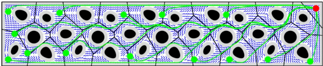
Fig. 4.Example navigation trajectories of the “move-to-projected-goal” law in (10) starting at a set of initial positions (green) far away from the goal (red).15

Work now in progress targets a fully smoothed version of the move-to-projected-goal law (by recourse to reference governors [43]), permitting its lift to more compli-cated dynamical models such as force-controlled (second-order) and underactuated sys-tems [44]. This will enable its empirical demonstration for safe, high-speed navigation in a forest-like environments [45] and in human crowds. We are also investigating the extension of these ideas for coordinated, decentralized feedback control of multirobot swarms. More generally, we seek to identify fundamental limits on navigable environ-ments for a memoryless greedy robotic agent with a limited range sensing capability.

Acknowlegdment. This work was supported by AFOSR under the CHASE MURI FA9550-10-1-0567.

References

1. Trautman, P., Ma, J., Murray, R.M., Krause, A.: Robot navigation in dense human crowds: Statistical models and experimental studies of humanrobot cooperation. The International Journal of Robotics Research34(3) (2015) 335–356

2. Henry, P., Vollmer, C., Ferris, B., Fox, D.: Learning to navigate through crowded environ-ments. In: Robotics and Automation, IEEE International Conference on. (2010) 981–986 3. Karaman, S., Frazzoli, E.: High-speed flight in an ergodic forest. In: Robotics and

Automa-tion (ICRA), IEEE InternaAutoma-tional Conference on. (2012) 2899–2906

4. Paranjape, A.A., Meier, K.C., Shi, X., Chung, S.J., Hutchinson, S.: Motion primitives and 3D path planning for fast flight through a forest. The Int. J. Robot. Res.34(3) (2015) 357–377 5. Wooden, D., Malchano, M., Blankespoor, K., Howardy, A., Rizzi, A.A., Raibert, M.:

Au-tonomous navigation for BigDog. In: IEEE Int. Conf. Robot. Autom. (2010) 4736–4741 6. Johnson, A.M., Hale, M.T., Haynes, G.C., Koditschek, D.E.: Autonomous legged hill and

stairwell ascent. In: Safety, Security, and Rescue Robotics (SSRR), IEEE International Sym-posium on. (2011) 134–142

7. Choset, H., Lynch, K.M., Hutchinson, S., Kantor, G.A., Burgard, W., Kavraki, L.E., Thrun, S.: Principles of Robot Motion: Theory, Algorithms, and Implementations. MIT Press (2005) 8. LaValle, S.M.: Planning Algorithms. Cambridge University Press, Cambridge, U.K. (2006) 9. Koditschek, D.E., Rimon, E.: Robot navigation functions on manifolds with boundary.

Ad-vances in Applied Mathematics11(4) (1990) 412 – 442

10. Khatib, O.: Real-time obstacle avoidance for manipulators and mobile robots. The Interna-tional Journal of Robotics Research5(1) (1986) 90–98

11. Koditschek, D.E.: Exact robot navigation by means of potential functions: Some topological considerations. In: Robotics and Automation, IEEE International Conference on. (1987) 1–6 12. Rimon, E., Koditschek, D.E.: Exact robot navigation using artificial potential functions.

Robotics and Automation, IEEE Transactions on8(5) (1992) 501–518

13. Lionis, G., Papageorgiou, X., Kyriakopoulos, K.J.: Locally computable navigation functions for sphere worlds. In: Robotics and Automation, IEEE Int. Conf. on. (2007) 1998–2003 14. Filippidis, I., Kyriakopoulos, K.J.: Adjustable navigation functions for unknown sphere

worlds. In: Decision and Control and European Control Conference (CDC-ECC), IEEE Conference on. (2011) 4276–4281

15. Burridge, R.R., Rizzi, A.A., Koditschek, D.E.: Sequential composition of dynamically dexte-rous robot behaviors. The International Journal of Robotics Research18(6) (1999) 535–555 16. Conner, D.C., Choset, H., Rizzi, A.A.: Flow-through policies for hybrid controller synthesis

applied to fully actuated systems. Robotics, IEEE Transactions on25(1) (2009) 136–146 17. Choset, H., Burdick, J.: Sensor-based exploration: The hierarchical generalized Voronoi

18. Boyd, S., Vandenberghe, L.: Convex Optimization. Cambridge University Press (2004) 19. Arslan, O., Koditschek, D.E.: Exact robot navigation using power diagrams. In: Robotics

and Automation (ICRA), IEEE International Conference on. (2016) 1–8

20. Aurenhammer, F.: Power diagrams: Properties, algorithms and applications. SIAM Journal on Computing16(1) (1987) 78–96

21. Webster, R.: Convexity. Oxford University Press (1995)

22. ´O’D´unlaing, C., Yap, C.K.: A retraction method for planning the motion of a disc. Journal of Algorithms6(1) (1985) 104 – 111

23. Cort´es, J., Martınez, S., Karatas, T., Bullo, F.: Coverage control for mobile sensing networks. Robotics and Automation, IEEE Transactions on20(2) (2004) 243–255

24. Kwok, A., Martnez, S.: Deployment algorithms for a power-constrained mobile sensor net-work. International Journal of Robust and Nonlinear Control20(7) (2010) 745–763 25. Pimenta, L.C., Kumar, V., Mesquita, R.C., Pereira, G.A.: Sensing and coverage for a network

of heterogeneous robots. In: Decision and Control, IEEE Conference on. (2008) 3947–3952 26. Arslan, O., Koditschek, D.E.: Voronoi-based coverage control of heterogeneous disk-shaped robots. In: Robotics and Automation, IEEE International Conference on. (2016) 4259–4266 27. Okabe, A., Boots, B., Sugihara, K., Chiu, S.N.: Spatial Tessellations: Concepts and

Appli-cations of Voronoi Diagrams. 2nd edn. Volume 501. John Wiley & Sons (2000)

28. Haralick, R.M., Sternberg, S.R., Zhuang, X.: Image analysis using mathematical morphol-ogy. Pattern Analysis and Machine Intelligence, IEEE Transactions on9(4) (1987) 532–550 29. Munkres, J.: Topology. 2nd edn. Pearson (2000)

30. Kozlov, M., Tarasov, S., Khachiyan, L.: The polynomial solvability of convex quadratic programming. USSR Comp. Mathematics and Mathematical Physics20(5) (1980) 223–228 31. Bullo, F., Cort´es, J., Martinez, S.: Distributed Control of Robotic Networks: A Mathematical

Approach to Motion Coordination Algorithms. Princeton University Press (2009)

32. Rockafellar, R.: Lipschitzian properties of multifunctions. Nonlinear Analysis: Theory, Methods & Applications9(8) (1985) 867–885

33. Kuntz, L., Scholtes, S.: Structural analysis of nonsmooth mappings, inverse functions, and metric projections. Journal of Math. Analysis and Applications188(2) (1994) 346–386 34. Shapiro, A.: Sensitivity analysis of nonlinear programs and differentiability properties of

metric projections. SIAM Journal on Control and Optimization26(3) (1988) 628–645 35. Liu, J.: Sensitivity analysis in nonlinear programs and variational inequalities via continuous

selections. SIAM Journal on Control and Optimization33(4) (1995) 1040–1060

36. Chaney, R.W.: PiecewiseCk_{functions in nonsmooth analysis. Nonlinear Analysis: Theory,} Methods & Applications15(7) (1990) 649 – 660

37. Khalil, H.K.: Nonlinear Systems. 3rd edn. Prentice Hall (2001)

38. Paternain, S., Koditschek, D.E., Ribeiro, A.: Navigation functions for convex potentials in a space with convex obstacles. IEEE Transactions on Automatic Control (submitted) 39. Holmes, R.B.: Smoothness of certain metric projections on Hilbert space. Transactions of

the American Mathematical Society184(1973) 87–100

40. Fitzpatrick, S., Phelps, R.R.: Differentiability of the metric projection in Hilbert space. Transactions of the American Mathematical Society270(2) (1982) 483–501

41. Hirsch, M.W., Smale, S., Devaney, R.L.: Differential Equations, Dynamical Systems, and an Introduction to Chaos. 2nd edn. Academic Press (2003)

42. Stewart, J.: Calculus: Early Transcendentals. 7th edn. Cengage Learning (2012)

43. Kolmanovsky, I., Garone, E., Cairano, S.D.: Reference and command governors: A tutorial on their theory and automotive applications. In: American Control Conf. (2014) 226–241 44. Arslan, O., Koditschek, D.E.: Smooth extensions of feedback motion planners via reference

governors. In: (submitted to) Robotics and Automation (ICRA), IEEE Int. Conf. on. (2017) 45. Vasilopoulos, V., Arslan, O., De, A., Koditschek, D.E.: Minitaur bounds home through a