Dissertations and Theses
6-2015
Sensor Fusion and Obstacle Avoidance for an Unmanned Ground
Sensor Fusion and Obstacle Avoidance for an Unmanned Ground
Vehicle
Vehicle
Gurasis Singh
Follow this and additional works at: https://commons.erau.edu/edt
Part of the Aerospace Engineering Commons Scholarly Commons Citation
Scholarly Commons Citation
Singh, Gurasis, "Sensor Fusion and Obstacle Avoidance for an Unmanned Ground Vehicle" (2015). Dissertations and Theses. 248.
https://commons.erau.edu/edt/248
This Thesis - Open Access is brought to you for free and open access by Scholarly Commons. It has been accepted for inclusion in Dissertations and Theses by an authorized administrator of Scholarly Commons. For more
SENSOR FUSION AND OBSTACLE AVOIDANCE FOR AN UNMANNED GROUND VEHICLE
A Thesis
Submitted to the Faculty of
Embry-Riddle Aeronautical University by
Gurasis Singh
In Partial Fulfillment of the Requirements for the Degree
of
Master of Science in Aerospace Engineering
June 2015
Embry-Riddle Aeronautical University Daytona Beach, Florida
2
Acknowledgements
It provides for me colossal joy to recognize the individuals who gave me the vital directions, help and ceaseless inspiration towards the fulfillment of this preposition.
I would like to augment my appreciation and exceptionally recognize my advisor, Dr. Richard J. Prazenica for his specialized direction, supervision and consistent good backing amid the course of this postulation. He empowered me to strike the right harmony in the middle of classes and theory work, investigate the flexible character implanted in me and yield a quality output at all times.
I would like to thank Dr. Hever Moncayo for serving on the panel and for furnishing me with quality specialized information throughout the span of this postulation.
I owe my deepest gratitude to Dr. Sathya Gangadharan for serving on the panel and for giving fundamental direction and backing in the midst of his occupied calendar.
I would like to share this achievement with my mother Manjit Kaur, my father Jaswinder Singh and my sister Manmeet and thank them for their love, motivation, support and faith in me.
I would like to express deep appreciation towards my friends Navroz Lamba and Abhinandan for their support and encouragement throughout my thesis work.
Finally, I would like to share this feat with my Uncle Dr. Bp Sodhi and my aunt Sharon Sodhi and express my sincere appreciation for their never-ending love, continual motivation and strong support extended at all times.
3
ABSTRACT
Author: Gurasis Singh
Title: Sensor Fusion and Obstacle Avoidance for an Unmanned Ground Vehicle
Institution: Embry-Riddle Aeronautical University
Degree: Master of Science in Aerospace Engineering
Year: 2015
In recent years, the capabilities and potential value of unmanned autonomous systems (UAS) to perform an extensive variety of missions have significantly increased. It is well comprehended that there are various challenges associated with the realization of autonomous operations in complex urban environments. These difficulties include the requirement for precision guidance and control in conceivably GPS-denied conditions as well as the need to sense and avoid stationary and moving obstructions within the scene. The small size of some of these vehicles restricts the size, weight and power consumption of the sensor payload and onboard computational processing that can accommodated by UAS.
This thesis analyzes the development and implementation of terrain mapping, path planning and control algorithms on an unmanned ground vehicle. Data from GPS, IMU and LIDAR sensors are fused in order to compute and update a dense 3D point cloud that is used by an implicit terrain algorithm to provide detailed mathematical representations of
4
complex 3D structures generally found in urban environments. A receding horizon path planning algorithm is employed to adaptively produce a kinematically-feasible path for the unmanned ground vehicle. This path planning algorithm incorporates obstacle avoidance constraints and provides a set of waypoints to be followed by the unmanned ground vehicle. A waypoint controller is designed and implemented to enable the vehicle to follow the waypoints from the path planner. Open-loop experiments are provided with an unmanned ground vehicle in order to demonstrate terrain generation with real sensor data. Closed-loop results are then presented for a simulated ground vehicle in order to demonstrate the performance of the receding horizon path planning and control algorithms using the terrain map generated from the open-loop experiments.
5
Contents
1) Introduction………12
1.1
Terminology………...12
1.2
Motivation………..12
1.3
Literature Review………..13
1.4
Existing Autonomous Vehicles……….16
1.4.1
Military Applications………...16
1.4.2
Consumer Applications………17
1.5
Technical objectives………..18
1.6
Organization of thesis………...21
2) Unmanned Ground Vehicle and Sensors……….22
2.1 Unmanned Ground Vehicle...………...22
2.2GPS receiver………...25
2.3IMU………27
6
3) Data Processing and Sensor fusion………...………30
3.1 Reference Frames……….….30
3.2 Coordinate Transformation………..32
3.3 Position Calculations……….…………....35
3.3.1 Computing the initial GPS location in ECEF frame….………37
3.3.2 Local NED frame coordinate transformation…………...….…37
3.3.3 Locating the origin of Local NED frame………..39
3.3.4 Expressing the GPS Position in local NED frame………40
3.4 INS Orientation Calculations...……….…………..40
3.5 LIDAR Point Cloud Calculations……..……….41
4) Terrain Mapping and Path Planning……….….…..43
4.1 3D Implicit terrain representation from point cloud…………43
4.2 Receding Horizon Path Planning Algorithm……….47
5) Modeling and Control of Unmanned Ground Vehicles……….…..54
5.1 UGV Kinematics………...54
7
6) Experimental and Simulation Results……….……….62
6.1 Open-Loop Experiment Measurements 1………...62
6.2 Open-Loop Experiment Measurements 2………...73
6.3 Closed-Loop Simulation Results…....……….82
7) Conclusions………..97
7.1 Concluding Remarks………...94
7.2 Future Work………94
Bibliography………...96
8
List of Figures
1.1 Overview of an autonomous System for UGV………..20
2.1a Corobot Unmanned Ground Vehicle ………..24
2.1b Left Side Power Selector Switch and power connectors………...24
2.1c Ride Side Power and Reset Buttons……….………24
2.1d Rear view of the Corobot……….25
2.2 Global Sat BU-353GPS receiver………....26
2.3 3D GX3-45 GPS Aided Inertial Navigation System………...28
2.4 Hokuyo UTM-30 LX LIDAR……….29
3.1 Different Frames of Reference………...31
3.2 Rotation about axis by yaw angle………...32
3.3 Rotation about axis by Pitch angle………...33
3.4 Rotation about axis by roll angle..………...33
3.5a Earth Center Earth Fixed (with origin at center of Earth)……….………35
3.5b the longitude from overhead view of Earth………...36
3.5c The Geodetic Latitude and altitude from side of earth…….……….36
3.6 Rotation about e axis by individual longitude………...38
9
4.1 Effect of Varying the isolevel Parameters……….47
4.2 Candidate Path Points for two dimensional path planning………....49
4.3 Path Planning Scenario (Goal location B)………...51
5.1 Differential Drive Kinematics………54
5.2 Feedback control law of Ground Robot…...57
5.3 Waypoint Controller………..………...58
5.4 Position of Robot at different time intervals……….………..61
6.1.1 View of overall path from Camera on UGV………...63
6.1.2 View of the overall path taken at ERAU campus (shown in red)………64
6.1.3 Zoomed in view of figure 5.1.2………64
6.1.4 Ground Vehicle Track with sample images from camera on UGV……….65
6.1.5 LIDAR measurements with vehicle path (Shown in Red)………...66
6.1.6 GPS measurement………66
6.1.7 NED Position of the vehicle CM………..67
6.1.8 Orientation Measurements………...67
6.1.9 3D representations at different time intervals………..69
6.1.10 Complete 3D terrain representation with Vehicle path………..69
10
6.1.12 Effect of Varying Isolevel Parameter……….72
6.2.1 View of overall Path………...73
6.2.2 View of Overall Path from google earth………..………74
6.2.3 Ground Vehicle Track with Sample Images from camera mounted mounted…….74
6.2.4 LIDAR measurements with path shown in red………75
6.2.5 NED position of the vehicle CM………..75
6.2.6 GPS measurements from Global Sat BU-353………..76
6.2.7 Orientation measurements from Micro strain………..76
6.2.8 3D terrain representation (Vehicle path shown in red)………...79
6.2.9 Overhead view of 3D terrain representation with path (shown in red)………79
6.2.10 Oblique view of 3D terrain representation……….80
6.2.11 3D view of terrain representation by 3D implicit terrain algorithm………80
6.2.12 Alternative view of the full 3D terrain representation………….…...81
6.3.1 Overall Path Scenario with Target location…….………...81
6.3.2 Receding Horizon Decisions at several Points…...89
11
CHAPTER 1 Introduction
1.1
Terminology
The meaning of autonomous is somewhat unclear and open to much debate. This work will describe an autonomous vehicle as a mobile robot that can explore and operate within an urban environment with minimal human cooperation. Terms such as robot and intelligence have a wide range of implications. These terms will be characterized in order to define the autonomous vehicle examined in this work. The term robot evokes various images. The movie industry has made robots popular and depicts the concept of robots in numerous motion pictures such as Iron man, Dhoom2 and Transformers. However these mythical cases are not an accurate representation of the robots that presently exist and work today.
For this research, the term robot will depict an unmanned ground vehicle (UGV). The autonomous UGV gathers information from onboard sensors, processes these data and then reacts to this information. To an outside observer, the robot would appear to be autonomously making decisions focused around the circumstances it experiences in its surroundings.
1.2
Motivation
Urban pursuit and related missions impose unique requirements on autonomous systems frameworks. Since an outside communication link is not always available or practical for providing control commands to the vehicle, unmanned vehicles must have the capacity to operate autonomously. In particular, the constrained payload available to small aerial systems poses a great challenge to the system design. A tradeoff between flight
12
execution, sensors and processing assets must be found. Since communication with these unmanned system cannot be assured at all times, sensor process and decision making must be done onboard for successful operation in obstacle strewn environments such as hilly terrain, woodlands or urban areas. These capabilities require the incorporation of sensing and control methodologies for obstacle avoidance, path planning and control that consider the complexities of the whole UAV system.
1.3
Literature Review
Over the previous decades, UAVs have been progressively utilized for an extensive array of applications [1]; for example observation, reconnaissance, surveying and mapping, spatial data securing, and geophysics investigations. Therefore, the navigation of unmanned aerial vehicles is of considerable interest. The limited payload of small aerial system poses a great challenge to the system design. The Global Positioning System (GPS) is an essential navigational sensor modality utilized for the vehicle direction and guidance [7, 8]. Nonetheless, a comprehensive study alluded to as the Volpe report [9] discusses vulnerabilities of GPS related with signal interruptions. These interruptions can be caused by RF interference, ionosphere interference, jamming or spoofing. This report inspired many strategies to mitigate the vulnerabilities of the current GPS navigation convention. Another widely used navigation sensor used for calculating the position of the vehicle [10-13] is the IMU (inertial measurement unit). It is composed of accelerometers, magnetometers and angular rate sensors. Accelerometers measure the sum of linear acceleration, typically in three orthogonal axes, due to the vehicle motion and the acceleration due to gravity. The direction of the local magnetic field is measured by magnetometers. A measure of the three dimensional rate of rotation of the body (i.e.,
13
angular velocity) is provided by angular rate sensors. An orientation estimate is typically computed using the direction of the earth’s gravitational and magnetic vector along with the angular rates, but there are drawbacks associated with using an IMU alone for navigation. First, there is quadratic growth in position drift error due to the double integration of acceleration data containing bias and random noise. Similarly, the integration of angular rate data to estimate orientation is also subject to the accumulation of drift error. To mitigate these errors, IMU are commonly fused with GPS in a navigation filter, providing improved accuracy. An inertial navigation system (INS) with GPS depends on the quality of the GPS signal but the GPS signal can be vulnerable to interference and spoofing as discussed earlier. Therefore, alternative navigational sensors are of interest for GPS-denied navigation. In addition, alternative sensing modes are required in order to sense and avoid obstacles within complex operational environments.
Recently, airborne and space-based laser altimetry has developed as a promising strategy to capture precise digital elevation data with LIDAR sensors. An ever increasing range of applications has taken advantage of the high accuracy and dense sampling provided by LIDAR sensors, which have the advantages of low computational load and high processing rates [22-25]. Moreover, LIDAR is not constrained by lighting conditions. These sensors, therefore, have been employed to form dense point clouds for different applications [28, 29, and 30]. A 3D point cloud can be used by different methodologies to map the environment and to provide obstacle avoidance constraints. Some collision avoidance methods for UAVs are based on potential field methods that model obstacles as repellants and waypoints as attractors [32, 33]. Considerable research has been done on the problem of obstacle avoidance for mobile ground robots [34, 35]. For collision free
14
robot guidance, two safety properties: passive safety (no collision can happen when the robot moves) and strong passive safety (the robot further maintains sufficient maneuvering distance from obstacles to avoid collisions) were studied [35]. In another work, the point cloud from LIDAR sensors was used to generate 3D mathematical representations that basically provide the information about the obstacles in the environment [37].
Many algorithms have been tested for path planning of autonomous vehicles. These are categorized as path planning and trajectory planning algorithms. Path planning entails generating an obstacle free path to avoid collision based on set of criteria [38, 39]. Trajectory planning plans the movement of the robot along the planned path. One path planning approach that is receiving considerable attention in the literature is receding horizon control. The receding horizon methodology has the ability to incorporate obstacle avoidance constraints as well as input and state constraints. The receding horizon algorithm solves an optimal control problem over a finite time horizon, after which a new optimal control problem is solved. This process continues until the objective is achieved. Therefore, the receding horizon algorithm provides the ability to incorporate new data into the planning and control of the vehicle. The stability of receding horizon control methods requires careful consideration compared with conventional (infinite horizon) optimal control approaches, but is now a well understood issue [40].
There are many examples in which receding horizon methods were employed to plan and control the trajectory of the autonomous vehicles [41, 42]. An important characteristic feature of the receding horizon method is that it involves re-planning after short time intervals, making it possible to consider new information frequently. In another work, this approach was employed to plan the movement of an autonomous UAV along a
15
2D straight line path avoiding obstacles by re-planning every time it received new data [43]. In the majority of the above studies, the obstacles are assumed to be known a priori or estimated online by an obstacle detection algorithm.
1.4
Existing Autonomous vehicles
The two main applications of UAVs or UGVs are military use and civilian use.
1.4.1 Military Applications
In the previous decade, because of world conflicts and the quick progression of innovation, there has been an extraordinary military interest in self-governing or autonomous vehicles. In the future, the U.S. military would like to have a large portion of its battle force provided by unmanned independent vehicles. Autonomous vehicles are a favored weapon system because of their productivity, information accumulation capacities and assurance of human life. UAVs have the potential to perform intelligence, surveillance and reconnaissance (ISR) missions. Their application has extended to electronic assault, strike mission, concealment and demolition of enemy air resistance (SEAD/DEAD), battle pursuit and salvage (CSAR).
Two well-known unmanned aerial vehicles are the U.S. Air Force’s Predator and Global Hawk. The Predator is intended to provide steady discernment, reconnaissance and surveillance. This UAV is controlled from a ground control station (GCS), through a satellite connection, from it is given missions by a human operator. While the Predator has the ability to perform battle missions, a human operator makes an official determination to fire on a target. The Predator’s capacity to assault ground targets and protect troops from danger has demonstrated its value to the U.S. military [3]. Another example, the Global Hawk, is solely an observation and surveillance UAV that was assembled for high altitude,
16
long endurance missions. Furnished with complex radar and sensing systems, it can supply responsive and persistent information from many places inside enemy territory, day or night, with little concern for climate [4].
Autonomous vehicles are likewise being utilized at sea by the U.S. Navy and on the ground by the U.S. Army. Providing a ground vehicle with the ability to adjust to its surrounding and maintain strategic distance from obstructions is a challenging task.
1.4.2 Consumer Applications
As innovation advances and becomes less expensive, the number of applications of autonomous vehicles will increase. As a rule with innovation, what was at one time a top of the line, top secret military application eventually enters the commercial market in a totally distinctive capacity. As an example , the global positioning system (GPS) was created in the 1970’s entirely for the military but today is broadly utilized for automobile navigation, mail and bundle following and many other commercial applications. A similar trend is occurring with autonomous vehicles. For example, Roomba is an autonomous vacuum cleaner designed and made by iRobot, which costs around $250. iRobot claims Roomba can keep a house vacuumed with next to no human intervention. Another example of a civilian autonomous robot is Robomower. Friendly Robotics asserts that a customer can schedule the Robomower to cut their yard when desired [6]. These products seem at face value to be extraordinary answers for unremarkable assignments but there are issues with both of them. Lamentably, both of these items fail to meet expectations. They are not particularly clever machines. For example, both these robots explore their surroundings in an irregular manner. They make headway until they experience an obstruction, then they make a turn arbitrarily and proceed until another obstruction is
17
encountered. In a basic domain, for example a rectangular room or a round yard with few obstructions, this strategy can be effective. In complex environments, however, these systems end up being wasteful and ineffective. Surveys of these robots assert that when they were utilized in complex world settings, they would end up not vacuuming the entire room or leaving portions of grass unmowed. Clearly a superior guidance approach must be concocted for these scenarios.
1.5
Technical Objectives
This thesis emphasizes the system integration of algorithms for sensor fusion, mapping, path planning and controls for an unmanned ground vehicle (UGV) operating in a complex urban environment, with future extensions to an unmanned air vehicle (UAV). A key objective of the thesis is to provide a systems-level investigation of the different component algorithms required in the closed-loop system. These algorithms include sensor fusion to generate navigation and point cloud data, 3D implicit terrain representations of the scene, receding horizon path planning with obstacle avoidance constraints and a waypoint controller to enable the vehicle to follow the planned path. The following objectives are achieved in this thesis:
1) Generate detailed navigation data from the unmanned ground vehicle using IMU and GPS sensors.
2) Create a 3D point cloud from processed LIDAR data and generate a 3D representation of the environment using 3D implicit terrain algorithms.
3) Implement a receding horizon algorithm to adaptively plan a path through the scene while enforcing obstacle avoidance constraints provided by the 3D terrain map.
18
4) Develop and implement a UGV controller to enable the UGV to follow the planned waypoints.
5) Perform open-loop experiments with data collected from a UGV operating in a complex environment as well as closed-loop simulations of a UGV model navigating in a complex scene.
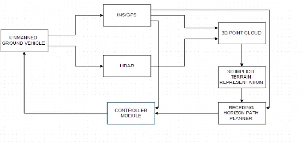
Figure 1.1: - Overview of an Autonomous System for UGV
The vehicle would commonly be instrumented with one or more traditional navigation sensors such as inertial measurement unit (IMU) (i.e. accelerometers and rate gyros) and GPS unit. A typical UAS payload might also incorporate a laser rangefinder or a line-scan LIDAR unit. Because the vehicle has an onboard LIDAR or rangefinder, a point cloud can be produced from LIDAR measurements and an estimate of the inertial position and orientation of the vehicle. The 3D point cloud, which is computed in an inertial reference frame, is utilized to produce a detailed 3D terrain map, which gives obstacle avoidance constraints to receding horizon path planner. The receding horizon module computes the path points that minimize a cost functional over a finite time horizon
19
while incorporating obstacle avoidance constraints. The control is connected over a subset of this horizon after which another optimization problem is performed to generate the next set of path points for the vehicle. Along these lines, the receding horizon methodology can incorporate new data from the updated obstacle map in the next path planning iteration. A controller is designed to drive the robot to the points planned by the receding horizon algorithm to reach its target point. The controller receives new waypoints at every time interval until the goal is achieved.
1.6
Organization of this Thesis
This thesis is organized as follows:
Chapter 2 discusses the unmanned ground vehicle (UGV) and sensors used in this research.
Chapter 3 provides details about the different reference frames and coordinates transformation required for navigation and the sensor fusion algorithms used to generate a LIDAR based point cloud.
Chapter 4 discusses the implicit terrain algorithms used to represent 3D urban terrain features based on LIDAR measurements and also provides the formulation of the receding horizon path planning algorithm with obstacle avoidance constraints.
Chapter 5 introduces a simulation model of the ground robot and develops a waypoint controller in order to navigate the vehicle to follow the planned path.
Chapter 6 provides open-loop experimental results in which these algorithms have been applied to data gathered from the UGV sensors as it traveled through
20
a complex scene. Closed–loop simulations are then provided and the performance of the algorithms is discussed
21
CHAPTER-2
Unmanned Ground Vehicle and Sensors
This chapter provides a detailed description of the unmanned ground vehicle and onboard sensor suite that was employed in this research. The sensor suite includes a MicroStrain 3DM-GX3-45 inertial navigation system (INS), a Hokuyo UTM-30LX line-scan LIDAR unit, and a Global sat BU-353 GPS receiver. Data from these sensors were fused to estimate the inertial position and orientation of the vehicle and to compute a 3D point cloud from which a terrain map of the environment was adaptively generated.
2.1 Unmanned Ground Vehicle
The unmanned ground vehicle is a completely robotized vehicle that can travel on a specific predefined course with minimal human intercession. The ground vehicle used in this work is a Corobot four wheeled robot that has an onboard computer. Figure 2.1 shows several views of the Corobot unmanned ground vehicle.
22
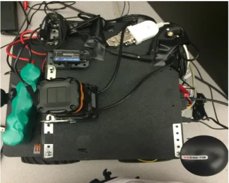
Figure 2.1b: Top view of the Corobot with sensors
The Corobot is instrumented with sensors, which are integrated with its hardware in order to record and process the sensor measurements. The ultimate goal is to enable the Corobot to operate autonomously in urban environments using the current position and desired waypoints generated by the receding horizon path planning algorithm. A controller (discussed later) is designed to generate commands to the motors in order to move the robot towards the next desired waypoint. The Corobot is Linux and Windows compatible, and Linux is required to be set up for the initial use. The sensors are integrated with the Corobot using Robot Operating System (ROS). The Corobot is intended for simple access, dismantling and reassembly for including and changing of equipment and parts. Because of its open structure, the Corobot is sensitive to debris. Operation under outdoor lighting conditions should represent no issue to the Corobot; however water will cause damage because the unit is not waterproof. The Corobot can connect to a local wireless network, which enables communication with the robot from a networked desktop, laptop or,
23
depending on network connections, from anywhere on the Internet. To drive the Corobot, the Corobot control panel is interfaced with a keyboard or joystick. Figure 2.1b depicts an overhead view of the Corobot with the integrated sensor suite, and Figures 2.1c through 2.1e provide several other views of the vehicle.
Figure 2.1c: Left side power selector switch and power connectors
24
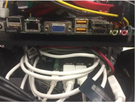
Figure 2.1e: Rear view of the Corobot
2.2 GPS Receiver
The global positioning system (GPS) is a space based global navigation satellite system that provides reliable positioning and time information in all weather and anywhere on or near the earth. GPS was established in 1973 by the U.S. Department of Defense. The GPS consists of a constellation of 27 earth orbiting satellites (24 in operation and three extra in case one fails). A GPS receiver locates four or more of these satellites, computes the distance to each satellite, and uses this information to deduce its location. The advantages of using GPS for navigation include its accuracy in determining position and the fact that GPS receivers are lightweight and inexpensive. A shortcoming of GPS is that the signal is often unavailable in urban and mountain areas, as well as indoor and underground environments. GPS signals are also vulnerable to interference and spoofing. They have a low update frequency, which is normally 1-10 Hz, which is 1-2 orders of magnitude lower than that of a standard INS.
25
Figure 2.2 GlobalSat BU-353 GPS receiver
The GPS receiver used for this work is the GlobalSat BU-353. This GPS receiver has the following features:
1) Its bottom is non slippery and waterproof
2) It has the capability to predict satellite position for up to 3 days in advance 3) Low power consumption
4) It has a built in patch antenna
Each row of the GPS data file corresponds to a position measurement. The data file has 4 columns corresponding to [Time stamp (ms), Geodetic Latitude 𝜆𝐷(deg), Longitude
𝜑𝐷(deg), Altitude h (m)]. Note that the GPS measurement provides position relative to the WGS-84 ellipsoid. Therefore, the altitude is approximately equivalent to height above sea level.
2.3 Inertial Navigation System
An inertial navigation system (INS) is an electronic device that uses a combination of accelerometers, gyroscopes, GPS, and magnetometers to measure the vehicle’s position, velocity, orientation and angular velocity. The INS contains an inertial measurement unit (IMU), which measures acceleration utilizing one or more accelerometers and measures
26
rotation using one or more rate gyroscopes. Furthermore, many INS incorporate magnetometer data in a navigation filter in order to reduce drift in the orientation (i.e., roll, pitch, and yaw) angles that are calculated from integrating noisy rate gyro data. The position of the vehicle can be calculated directly from IMU data in a process known as dead reckoning, but typically GPS data are incorporated into a navigation filter to reduce drift in the position estimates. An advantage of IMU sensors is that their data sampling rate is high (on the order of 50 Hz) compared to that of GPS (on the order of 1-10 Hz).
For this thesis research, a Microstrain 3DM-GX3-45 INS sensor, as shown in Figure 2.3, was used. This INS consists of a triaxial accelerometer, a triaxial gyro, a triaxial magnetometer and a temperature sensor. It additionally has an installed processor that runs a navigation filter to provide static and dynamic orientation and inertial position estimates.
Figure 2.3 Microstrain 3DM-GX3-45 GPS Aided Inertial Navigation System
The 3D-GX3-45 provides a range of navigation related output quantities. Fully calibrated inertial measurements include acceleration, angular rates, magnetic field, delta theta and delta velocity vectors, Euler angles (pitch, roll and heading), rotation matrix and quaternion.
27
2.4 LIDAR
LIDAR (light detection and ranging) is a remote sensing innovation that measures 3D point clouds of the earth’s surface. Some airborne LIDAR instrumentation utilize a laser scanner with up to 400,000 pulses of light per second. At the point when an airborne laser is pointed at a focused region on the ground, the light emission is reflected by the surface. A sensor records this reflected light to measure the range. Laser range measurements are fused with vehicle position and orientation information in order to generate a dense, detail-rich collection of 3D elevation points known as a “point cloud.”
The LIDAR used in this work was the Hokuyo UTM-30 LX line-scan LIDAR, pictured in Figure 2.4. This line-scan sensor rotates the laser about a single axis in order to produce planar scans of the surrounding environment.
Figure 2.4 Hokuyo UTM-30LX Line-Scan LIDAR
Features of the Hokuyo UTM-30LX LIDAR include
1) Minimum range of 10 mm 2) Maximum range of 60 m
28 3) Scan angle of 270 degrees
4) Scan rate of 25 ms (40 scans/sec) 5) Mass of 210g
29
Chapter -3
Data Processing and Sensor Fusion
This chapter discusses the algorithms required for processing the GPS, INS, and LIDAR data in order to compute the position and orientation of the vehicle as well as generating a 3D point cloud. In order to construct a terrain map, the LIDAR measurements must be expressed in a common inertial reference frame. The computation of this LIDAR-based point cloud entails transforming the LIDAR measurements, which are collected with respect to the LIDAR sensor, to the inertial frame using the estimated position and orientation of the ground vehicle. The reference frames and coordinate transformations required for this analysis are also provided in this chapter.
3.1 Reference Frames
Several different reference frames are utilized in the sensor fusion algorithms discussed in this chapter. These reference frames, illustrated in Figure 3.1, include a local geodetic (North-East-Down) frame G, which for the purposes of this ground robot application serves as an inertial reference frame, a body reference frame B that is fixed within the vehicle (i.e., the coordinate axes move with the vehicle), and a sensor frame S that is fixed within each sensor.
30
Figure 3.1 Geodetic (NED), Body, and Sensor Reference Frames
In Figure 3.1, 𝑟⃗⃗⃗ 𝑏 represents the position of the vehicle center of mass (CM) relative to the origin of the inertial frame and 𝑟⃗⃗ 𝑠 denotes the position of the sensor relative to the vehicle CM. The coordinate axes of the geodetic, body, and sensor frames are defined as follows.
Local Geodetic (Inertial) Frame G 𝑔̂1 corresponds to local North 𝑔̂2 corresponds to local East 𝑔̂3 corresponds to local Down Body Fixed Frame B
Origin is located at the vehicle CM
𝑏̂1 is pointed out the front of the vehicle
𝑏̂2 is pointed out the right side of the vehicle
𝑏̂3 is pointed downward, completing the orthogonal triad Sensor Fixed Frame S
31
Origin is collocated with the LIDAR sensor
sˆ1 is pointed out the front of the sensor sˆ2 is pointed out the right side of the sensor
sˆ3 is pointed downward, completing the orthogonal triad
3.2 Coordinate Transformations
Given the reference frames defined in the previous section, it is necessary to define the coordinate transformations required to express data in these different reference frames. These coordinate transformations take the form of rotation matrices that transform data representations from one reference frame to another.
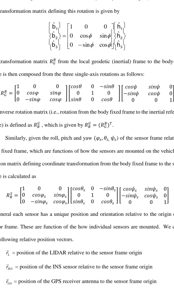
Given the measured roll φ, pitch θ, and yaw ψ of the vehicle, the rotation matrix
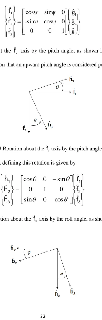
𝑅𝐺𝐵 defining the transformation from the geodetic (inertial) reference frame to the body-fixed reference frame is defined in terms of 3 single-axis rotations. The first of these is a rotation about the ĝ3 axis by the yaw angle, as shown in Figure 3.2. This rotation uses the usual convention that yaw is measured clockwise from the North.
Figure 3.2 Rotation about the ĝ3 (local down) axis by the yaw angle The transformation matrix defining this rotation is given by
32 1 1 2 2 3 3 ˆf cosψ sinψ 0 gˆ ˆ ˆ f = -sinψ cosψ 0 g ˆ 0 0 1 gˆ f
The next rotation is about the ˆf2 axis by the pitch angle, as shown in Figure 3.3. This rotation uses the convention that an upward pitch angle is considered positive.
Figure 3.3 Rotation about the fˆ1 axis by the pitch angle Ɵ
The transformation matrix defining this rotation is given by
3 2 1 3 2 1f
f
f
h
h
h
ˆ
ˆ
ˆ
cos
0
sin
0
1
0
sin
0
cos
ˆ
ˆ
ˆ
33
Figure 3.4 Rotation about the hˆ axis by the roll angle φ 1 The transformation matrix defining this rotation is given by
3 2 1 3 2 1 h h h b b b ˆ ˆ ˆ cos sin 0 sin cos 0 0 0 1 ˆ ˆ ˆ
The transformation matrix 𝑅𝐺𝐵 from the local geodetic (inertial) frame to the body-fixed frame is then composed from the three single-axis rotations as follows:
𝑅𝐺𝐵= [10 𝑐𝑜𝑠𝜑0 𝑠𝑖𝑛𝜑0 0 −𝑠𝑖𝑛𝜑 𝑐𝑜𝑠𝜑 ] [ 𝑐𝑜𝑠𝜃 0 −𝑠𝑖𝑛𝜃 0 1 0 𝑠𝑖𝑛𝜃 0 𝑐𝑜𝑠𝜃 ] [ 𝑐𝑜𝑠𝜓 𝑠𝑖𝑛𝜓 0 −𝑠𝑖𝑛𝜓 𝑐𝑜𝑠𝜓 0 0 0 1 ]
The inverse rotation matrix (i.e., rotation from the body fixed frame to the inertial reference frame) is defined as 𝑅𝐵𝐺 , which is given by 𝑅𝐵𝐺 = (𝑅𝐺𝐵)𝑇.
Similarly, given the roll, pitch and yaw (𝜑𝑠, 𝜃𝑠, 𝜓𝑠) of the sensor frame relative to body fixed frame, which are functions of how the sensors are mounted on the vehicle, the rotation matrix defining coordinate transformation from the body fixed frame to the sensor frame is calculated as 𝑅𝐵𝑆 = [10 𝑐𝑜𝑠𝜑0 0 𝑠 𝑠𝑖𝑛𝜑𝑠 0 −𝑠𝑖𝑛𝜑𝑠 𝑐𝑜𝑠𝜑𝑠] [ 𝑐𝑜𝑠𝜃𝑠 0 −𝑠𝑖𝑛𝜃𝑠 0 1 0 𝑠𝑖𝑛𝜃𝑠 0 𝑐𝑜𝑠𝜃𝑠 ] [ 𝑐𝑜𝑠𝜓𝑠 𝑠𝑖𝑛𝜓𝑠 0 −𝑠𝑖𝑛𝜓𝑠 𝑐𝑜𝑠𝜓𝑠 0 0 0 1 ]
In general each sensor has a unique position and orientation relative to the origin of the sensor frame. These are function of the how individual sensors are mounted. We define the following relative position vectors.
L
r = position of the LIDAR relative to the sensor frame origin
INS
r = position of the INS sensor relative to the sensor frame origin
GA
34
Defining references frame fixed to each individual sensor, the rotation matrices that define the transformation from the sensor fixed reference frame to the individual sensor frames can be defined in terms of the roll, pitch and yaw of each sensor relative to the sensor frame. These angles are a function of how each sensor is mounted. Therefore, we define the following rotation matrices.
𝑅𝑆𝐿(𝜑
𝐿,𝜃𝐿, 𝜓𝐿) = orientation of the LIDAR relative to the sensor frame
𝑅𝑆𝐼𝑁𝑆(𝜑
𝐼𝑁𝑆, 𝜃𝐼𝑁𝑆, 𝜓𝐼𝑁𝑆) = orientation of the INS sensor relative to the sensor frame
𝑅𝑆𝐺𝐴(𝜑
𝐺𝐴,𝜃𝐺𝐴, 𝜓𝐺𝐴) = orientation of the GPS antenna relative to the sensor frame In this ground vehcile application, the rotation matrix 𝑅𝐵𝑆 (rotation of body fixed frame to the sensor frame) reduces to the identity matrix because the sensors are mounted on the vehicle so they are aligned with the body fixed axes. For this work, the origin of sensor frame was selected to be collocated with the origin of the LIDAR. The LIDAR, INS, and GPS sensors are mounted with the same alignment; therefore, the rotation matrices (𝑅𝑆𝐿, 𝑅𝑆𝐼𝑁𝑆, 𝑅𝑆𝐺𝐴) all reduce to the identity matrix.
3.3 Position Calculations
The latitude, longitude and altitude are measured with respect to geodetic coordinates providing the position of the GPS receiver relative to the WGS-84 ellipsoid. An earth centered, earth fixed reference frame E can be defined at the center of the earth as follows:
35
Figure 3.5a Earth centered, earth fixed frame E (origin at center of Earth)
Figure 3.5b The longitude D from an overhead view of the Earth
36
Given the GPS measurements (geodetic latitude, longitude and altitude), it is desirable to compute the vehicle position with respect to a local geodetic (North, East, Down) reference frame. A NED reference frame can be defined from the initial GPS measurement (𝜆𝐷,0, 𝜑𝐷,0, ℎ0) by first expressing the initial GPS location in the Earth-centered, Earth-fixed (ECEF) frame. Then the rotation matrix that transforms the ECEF frame into a local NED frame can be defined, and the origin of the NED frame is located at the initial ECEF location of the vehicle center of mass. All subsequent GPS measurements can then be referenced to this local NED frame.
3.3.1 Computing the initial GPS position in the ECEF frame
The initial GPS location can be expressed in terms of the ECEF reference frame as follows:
0,GPS,ECEF 0 D,0 D,0a
X
=
+ h
cos λ
cos φ
χ
2
0,GPS,ECEF 0 D,0a
Z
=
1- e
+ h
sin λ
χ
wherea = 6378137 m (semi-major axis of the WGS-84 ellipsoid)
𝑒2= 0.00669438 (square of the eccentricity of the WGS-84 ellipsoid) χ = √1 − 𝑒2𝑠𝑖𝑛2(𝜆
𝐷,0)
3.3.2 Local NED Frame Coordinate Transformation
0,GPS,ECEF 0 D,0 D,0a
Y
=
+ h
cos λ
sin φ
χ
37
The rotation matrix 𝑅𝐸𝐺 defining the transformation from the ECEF reference frame to a local NED reference frame, where the North-East plane is tangent to the surface of the WGS-84 ellipsoid at the origin, can be defined in terms of three single-axis rotations. The first rotation is about the ECEF
3
ˆe
axis by the initial longitude 𝜑𝐷,0 as shown in Figure 3.6.Figure 3.6 Rotation about
3
ˆe
axis by initial longitude φD,0 The rotation about the3
ˆe
axis by the initial longitude 𝜑𝐷,0 is given by the following matrix:1 D,0 D,0 1 2 D,0 D,0 2 3 3 ˆ ˆ e cosφ sinφ 0 e ˆ ˆ e = -sinφ cosφ 0 e ˆ ˆ e 0 0 1 e
The next rotation corresponds to a rotation about the eˆ2 axis by the initial latitude 𝜆𝐷,0, which is given by the matrix
1 D,0 D,0 1 2 2 3 D,0 D,0 3 ˆ ˆ e cosλ 0 sinλ e ˆ ˆ e = 0 1 0 e ˆ ˆ e -sinλ 0 cosλ e
After the second rotation, we have an Up North East reference frame. In order to obtain a North East Down frame, the direction of the upward axis must be reversed and the
38
coordinate axes must be reordered. These operations are achieved by the following transformation: 1 1 2 2 3 3 ˆ ˆ g 0 1 0 e ˆ ˆ g = 0 0 1 e ˆ ˆ g -1 0 0 e
3.3.3 Locating the Origin of the Local NED Frame
The origin of the local NED frame is located at the position of the vehicle CM when the initial GPS measurement is taken. The position in the ECEF reference frame can be computed as
0,cm 0,GPS ECEF E G B E G B S 0,Cm 0,cm 0,GPS G 0,B S G 0,B S GA 0,cm ECEF 0,GPS ECEF X X r = Y = Y - R R r + R R R r Z Z Position of GPS w.r.t vehicle CM where𝑅𝑂,𝐵𝐺 = initial rotation from body-fixed to local NED reference frame (derived from the initial orientation angles)
B S
r = position of the sensor frame origin relative to the CM, expressed in the body-fixed reference frame.
𝑅𝑆𝐵 = rotation from sensor frame to body-fixed reference frame (computed from the mounting angles of the sensor box)
S GA
r = position of the GPS antenna relative to the sensor frame origin, expressed in the sensor reference frame.
39
The local NED position of the vehicle CM at each time step is computed by subtracting the position of the GPS antenna relative to the CM:
cm G G G B G B S CM cm GPS B S B S GA cm GX
r
= Y
= r
- R r + R R r
Z
where 𝑅𝐵𝐺 denotes the rotation from the body-fixed to the local NED reference frame, which is derived from the vehicle orientation angles at each time step.
3.4 INS Orientation Calculations
Orientation measurements are obtained from the Microstrain 3DM-GX3-45 INS sensor. The measurements (𝜑𝑚, 𝜃𝑚, 𝜓𝑚) provide the orientation of the INS sensor relative to the local geodetic (inertial) frame, from which we can then compute the orientation of the vehicle relative to the geodetic frame. The rotation matrix defining the transformation from the geodetic frame to the orientation sensor frame is computed as
𝑅𝐺𝐼𝑁𝑆 = [10 𝑐𝑜𝑠𝜑0 0 𝑚 𝑠𝑖𝑛𝜑𝑚 0 −𝑠𝑖𝑛𝜑𝑚 𝑐𝑜𝑠𝜑𝑚] [ 𝑐𝑜𝑠𝜃𝑚 0 −𝑠𝑖𝑛𝜃𝑚 0 1 0 𝑠𝑖𝑛𝜃𝑚 0 𝑐𝑜𝑠𝜃𝑚 ] [ 𝑐𝑜𝑠𝜓𝑚 𝑠𝑖𝑛𝜓𝑚 0 −𝑠𝑖𝑛𝜓𝑚 𝑐𝑜𝑠𝜓𝑚 0 0 0 1 ]
As mentioned previously, the origin of the sensor frame is collocated with the origin of the LIDAR sensor frame. Therefore, given the rotation matrices 𝑅𝑆𝐼𝑁𝑆(orientation of the INS frame relative to the sensor frame) and 𝑅𝐵𝑆 (orientation of the sensor frame relative to the body fixed frame), the rotation matrix describing the orientation of the body fixed frame relative to the local geodetic (NED) frame is given by
𝑅𝐺𝐵 = 𝑅
𝑆𝐵𝑅𝐼𝑁𝑆𝑆 𝑅𝐺𝐼𝑁𝑆
For this work, the INS sensor is aligned with the LIDAR, and the LIDAR is aligned with the vehicle. Therefore,
40 RBS = R INS S = I RBG= R 𝑮 INS
Hence, φ = 𝜑𝑚 , 𝜃 = 𝜃𝑚, and 𝜓 = 𝜓𝑚. That is, the vehicle orientation angles are equivalent to the orientation angles measured by the INS sensor.
3.5 LIDAR Point Cloud Calculations
The LIDAR reference frame is defined with the origin located on the LIDAR sensor. The LIDAR x axis (lˆ1 axis in Figure 3.5) is fixed along the sensor boresight, the y axis (lˆ2 axis in Figure 3.7) is pointed 90 degrees to the right of the sensor and the z axis is pointed downward (i.e., into the page).
Figure 3.7 LIDAR Reference Frame
Since the Hokuyo UTM-30LX is a line-scan LIDAR, all the measurements are in the lˆ1
-2 ˆ
l plane shown in Figure 3.7. The position vector of a LIDAR point measurement is given in the LIDAR reference frame as
az az ψ az P P L P ψ az P L d cos ψ x r = y = d sin ψ z 0 41 P G G G B G B S G B S L P P Cm B S B S L B S L P P G
X
r = Y
= r
+ R r + R R r + R R R r
Z
where G Cmr = position of the vehicle CM, expressed in the local geodetic (NED) reference
frame S L
r = position of the LIDAR relative to the sensor frame origin, expressed in the sensor reference frame (note that this is zero since the LIDAR frame is collocated with the sensor frame in this application)
𝑅𝐿𝑆 = rotation from the LIDAR reference frame to the sensor reference frame, derived from how the LIDAR is mounted relative to the sensor frame.
In this manner, each LIDAR point measurement is expressed in terms of a common reference frame, the local geodetic (NED) frame. This generates a dense collection of data points in the inertial frame, known as a point cloud, from which a 3D terrain map of the environment can be constructed.
42
Chapter 4
Terrain Mapping and Path Planning 4.1 3D Terrain Representations from Point Cloud Data
The point cloud generated from LIDAR measurements is used to generate a terrain representation of the environment. This thesis considers two methodologies that are based on mathematical learning theory developed by researchers at the University of South Carolina. Mathematical learning theory is a zone of parametric statistics that can be viewed as a converging of nonlinear approximation theory, adaptive tree algorithms and statistical estimation. A vital characteristic of learning algorithms is that they do not require information regarding the underlying probability distribution describing the full scenario. The first terrain mapping approach utilizes a mathematical learning algorithm to build adaptive, multiresolution terrain representations from point cloud data [36]. This approach generates a piecewise constant terrain representation over rectangular or triangular sub domains, but linear interpolation can be applied to obtain continuous piecewise linear representations. This approach is well suited for real time implementations because it is fast and recursive in nature. The only disadvantage with this approach is that it has tendency to cover the point cloud data with a terrain skin, which provides a functional representation that is not sufficient to represent certain 3D terrain features.
The second methodology uses implicit terrain algorithms to represent 3D features in the environment. It is able to represent 3D surfaces with a high level of detail; however, this algorithm is not recursive in nature (that is, the whole terrain representation must be regenerated every time new point cloud data are obtained). Basically, the implicit terrain algorithm fits a 3D isosurface around the point cloud data. The computation of the
43
isosurface is achieved by first producing a tetrahedral occupancy grid depending on the data distribution. An unsigned distance is then calculated from the cell vertices to the data within the cell in order to generate a 3D surface that embodies the data for each tetrahedral occupancy cell. The implicit terrain algorithms can be applied in navigation systems in order to generate representations of complex 3D terrain features. These algorithms are used to provide obstacle avoidance constraints to a receding horizon path planning algorithm.
The representation of the environment by these implicit terrain algorithms depends on three key parameters: the depth parameter, occupancy parameter and isolevel parameter. The depth parameter is used to describe the minimum size of the occupancy cells that will be used for the representation of the 3D terrain. The occupancy parameter defines the minimum number of data points that must occupy a cell before it is further subdivided into smaller cells. The isolevel parameter determines the distance of isosurface from the point cloud data. In other words, the isolevel parameter basically specifies the size of the isosurface that encapsulates the data. The isolevel parameter can be varied according to the resolution required to capture specific 3D terrain features since it provides the resolution of the complex 3D structure (that is, it specifies to what level of detail a particular feature can be resolved). A lower value of the isolevel parameter is better for the resolution of small features like people or vehicles, but it often results in holes or gaps in the terrain representations of larger structures such as buildings. Hence a higher value of the isolevel parameter is required for larger structures because it produces a smoother and more continuous surface, which best fits larger complex structures.
A test was performed to investigate the effect of varying the isolevel parameter on a specific point cloud data set, the results of which can be seen in Figure 4.1. This figure
44
shows the terrain representations obtained from LIDAR data collected from the unmanned ground vehicle as it traversed a path over relatively flat terrain. During this experiment, the vehicle passes between two orange traffic cones on either side of the path. The point cloud data were processed using the implicit terrain algorithm with isolevel parameters of 0.5 and 0.1.
45
(b) Terrain: Isolevel 0.1
46
(d) Terrain: Isolevel 1.0 (Different view)
Figure 4.1 Effect of Varying the Isolevel Parameter
It is clear from Figure 4.1 (c) and 4.1 (d) that a better resolution for small objects (cones) is obtained using a smaller value of the isolevel parameter, but the smaller isolevel parameter also results in gaps in the representation of the ground terrain (see Figure 4.1(b)). The larger isolevel provides better representations of larger structures or the full environment because it provides a smoother and more continuous terrain surface.
4.2 Receding Horizon Path Planning Algorithm
Receding horizon control (RHC), otherwise called model predictive control (MPC), is a modern control algorithm that started to receive considerable attention in the 1980’s. Essentially, with RHC, an optimization problem is solved over a finite time interval to determine a plan of action over a fixed time horizon. In RHC, the planner incorporates the
47
goal and constraints as components of an optimal control problem. RHC can also incorporate new information, constraints, future references and assessments of future disturbances. In this work, RHC is implemented as a path planning algorithm, which computes path points for the UGV that are passed to a waypoint controller.
The receding horizon path planning algorithm employed in this work computes a path that minimizes a mission based cost functional and incorporates obstacle avoidance constraints derived from the 3D terrain representation [43]. Therefore, with this approach, the vehicle travels a path that minimizes a cost function (low fuel consumption, minimum time of travel, etc.) subject to obstacle avoidance constraints. As discussed earlier, the RHC algorithm computes an optimal path over a finite time horizon. A part of this path is executed and meanwhile new information is accumulated by the sensors, the 3D terrain map is upgraded and a new optimal path is then computed. In this way, the vehicle path is planned over a sliding window in time until the vehicle attains its goal, which is a specified destination waypoint in this study. The autonomous navigation system is designed in such a manner that it generates the points or planned path to the control system, which in return generates the required control commands for the vehicle to follow the desired trajectory. Hence, in this work, RHC is used to generate a path that minimizes a cost functional subject to obstacle avoidance constraints derived from the 3D terrain map so that the vehicle can attain a target final waypoint.
48
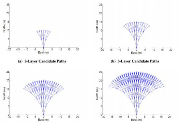
Figure 4.2 Candidate Path Points for Two-Dimensional Path Planning
The receding horizon path planning algorithm involves producing an arrangement of candidate path points for a certain interval of time and then determining the optimal sequence of path points within that horizon. Basically, the candidate points are arranged in a tree like structure such that there are different layers of points, and for moving from a point in one layer to another layer, there are multiple options available. In two dimensions, the important parameters are Np, Nc, 𝜓ℎand d, where Np is number of planned points, Nc
is number of path points to be followed, 𝜓ℎ is the maximum horizontal angle between the candidate points in the next layer and d is the distance between points in consecutive layers. Figure 4.2 shows the multiple layers of candidate 2D paths radiating from a vehicle situated at the origin and oriented due north. In this example, for every point in a given layer, there are 3 choices for moving to the following layer corresponding to heading changes of -15°,
49
0°, and 15°. Therefore, in this example, there is a 300 maximum horizontal angle (𝜓ℎ) between candidate points in the next layer with an angular resolution of 150, and the distance d is 5 meters between points in consecutive layers. With these parameters, there are a total of 3𝑁𝑝 candidate two-dimensional paths.
The augmentation of this approach to 3D is straightforward and involves selecting a maximum vertical path angle 𝜓𝑣 and a vertical angular resolution. If these two parameters are set equal to the horizontal angles as in the above scenario, there are 9 decisions from a given path point to the next and a total of 9𝑁𝑝 candidate paths. An important point to be noted here is that vehicle kinematic constraints can be applied through an appropriate choice of the path planning parameters. That is, the parameters can be chosen so that all candidate paths are within the maneuvering capabilities of the vehicle.
The mission objective of navigating the unmanned ground vehicle from a starting point A to a target location B can be cast as an optimization problem subject to path constraints for obstacle avoidance. The UGV equations of motion can be written as a system of nonlinear, coupled ordinary differential equations:
Ẋ (t) = F(X (t), U (t), t) (1) X (0) = 𝑋0
The vector X(t)represents the ground vehicle state vector and U(t) denotes the control input. Obstacles (i.e., the terrain map) are estimated from sensor measurements Y(t), given by
Y(t) = O (X(t); χ, t) (2) The observation operator O defines the output Y and its dependence on the vehicle states and the surrounding environment. The trajectory of the ground vehicle is constrained such
50
that it does intersect any obstacle within the environment. The symbol χ is used to express the subset of 𝑅3, three-dimensional space, occupied by obstacles. We denote
𝜒(X, Y, Z) =1 if (x, y, z) ∈ χ (3)
𝜒(X, Y, Z) = 0 otherwise Therefore, the path of the vehicle is subject to the constraint
(PX)(t) = (𝑋𝑐(𝑡), 𝑌𝑐(𝑡), 𝑍𝑐(t)) (4) In Eq. (4), P is an operator that selects specific states from the state vector X. This constraint enforces the requirement that the center of mass of the vehicle (𝑋𝑐, 𝑌𝑐, 𝑍𝑐), which is subset of the vehicle state vector, must not intersect any of the obstacles.
The receding horizon path planning algorithm associated with the objective of navigating the UGV from a starting point
XA,YA,ZA
to a goal location
XB,YB,ZB
is then formulated as the following optimization problem:Find the path points
i
H
k i k i k i k X Y Z k N
P , , , 1,, that minimize the cost functional
subject to the constraints
i k i k P P , 1 k = 1,…NH (obstacle avoidance) i k i kP k = 1,…NH (set of candidate path points)
A A A
i Z Y X P0 , , (initial condition) This optimization problem is solved from i = 0,…N, where N is the number of path planning steps required to reach the goal location B. After each path planning optimization, which provides NH path points, the first NC < NH path points are passed to a waypoint51
controller, which computes the control inputs required to drive the UGV through the path points. The UGV travels through the NC path points, during which time it collects new sensor data, updates the terrain map, and then solves a new optimization problem to compute the next set of path points. This process continues until the UGV reaches the goal location B.
Figure 4.3 Path Planning Scenario (Goal Location B)
This path planning algorithm was implemented by planning a series of trajectories using the receding horizon algorithm. This implementation minimizes a cost function that incorporates weighted terms for approaching the objective mission point B subject to obstacle avoidance constraints based on the 3D implicit terrain map. The obstacle avoidance constraints are implemented by first checking that, for every available path, the path points are no less than a distance 𝑑𝑠 from the from the 3D terrain surface, which indicates that the candidate path points are clear of obstacles by at least a margin of safety
𝑑𝑠. Then, all the paths that fulfill this requirement are ranked in order of increasing cost. Beginning with the minimal cost path, a higher resolution set of points is created along the
52
straight segments connecting the path points, and then the obstacle avoidance constraints are checked for each of these intermediate points. This procedure addresses the possibility that an obstacle may exist between two successive path points. If by chance none of the candidate paths fulfill these constraints, the algorithm returns a command to the vehicle to either stay in place to gather extra information or to change direction in an attempt to find a path that satisfies the requirements.
53
Chapter 5
Modeling and Control of the Unmanned Ground Vehicle
5.1 UGV Kinematics
The unmanned ground vehicle (UGV) used for this work is a differential drive robot with four wheels. The movement of the wheels on the same side of the vehicle is the same; hence for the ease of calculation, the equations of motions can be calculated for two tires representing either side of the vehicle. The two wheels are modeled as mounted on a common axis and can be moved independently in both the forward and backward directions. For the rolling motion of the robot, the velocity of each wheel can be varied but there must be common point for both wheels about which the robot can rotate. This point is called the instantaneous center of curvature.
54
The rate of rotation 𝜔 about the instantaneous center of curvature must be same for both the wheels. Hence we can write:
𝜔 (𝑅 +2𝑙) = 𝑉𝑟 5.1
𝜔(𝑅 − 𝑙/2) = 𝑉𝑙 5.2 where
l = distance between the center of the two wheels
𝑉𝑟 = translational velocity of the right wheel
𝑉𝑙 = translational velocity of the left wheel
R = distance from the instantaneous center of curvature to the midpoint between the wheels
c = instantaneous center of curvature From equation 5.1 and 5.2,
𝑅 = (
𝑙
2)(𝑉𝑙+𝑉𝑟)
(𝑉𝑙−𝑉𝑟) 5.3
𝜔 = (𝑉𝑙− 𝑉𝑟)/𝑙 5.4 From these equations, four cases can be derived:
1) If 𝑉𝑙= 𝑉𝑟, the robot moves in a straight line (linear motion) with no rotation. In this case, we obtain R and 𝜔 = 0.
2) If 𝑉𝑙 = −𝑉𝑟 , the vehicle rotates about the midpoint of the wheel axis. 3) If 𝑉𝑙= 0, the vehicle rotates about the left wheel in which case R = l/2. 4) If 𝑉𝑟= 0, the vehicle rotates about the right wheel in which case R = l/2.
The current position of the robot is denoted as (x, y) and the heading angle is defined as the angle between the position vector and the x axis. The values of 𝑉𝑙 and 𝑉𝑟