The Weight Function in the Subtree Kernel is Decisive

(1)

HAL Id: hal-02097593

https://hal.archives-ouvertes.fr/hal-02097593v2

Submitted on 22 Nov 2019

HAL is a multi-disciplinary open access archive for the deposit and dissemination of sci-entific research documents, whether they are pub-lished or not. The documents may come from teaching and research institutions in France or abroad, or from public or private research centers.

L’archive ouverte pluridisciplinaire HAL, est destinée au dépôt et à la diffusion de documents scientifiques de niveau recherche, publiés ou non, émanant des établissements d’enseignement et de recherche français ou étrangers, des laboratoires publics ou privés.

The Weight Function in the Subtree Kernel is Decisive

Romain Azaïs, Florian Ingels

To cite this version:

Romain Azaïs, Florian Ingels. The Weight Function in the Subtree Kernel is Decisive. 2019. �hal-02097593v2�

(2)

THE

WEIGHT

FUNCTION IN THE

SUBTREE

KERNEL IS

DECISIVE

Romain Aza¨ıs

[email protected]

Florian Ingels

[email protected]

Laboratoire Reproduction et D´eveloppement des Plantes, Univ Lyon, ENS de Lyon, UCB Lyon 1, CNRS, INRA, Inria, F-69342, Lyon, France

Abstract

Tree data are ubiquitous because they model a large variety of situations, e.g., the architecture of plants, the secondary structure of RNA, or the hierarchy of XML files. Nevertheless, the analysis of these non-Euclidean data is difficult per se. In this paper, we focus on the subtree kernel that is a convolution kernel for tree data introduced by Vishwanathan and Smola in the early 2000’s. More precisely, we investigate the influence of the weight function from a theoretical perspective and in real data applications. We establish on a 2-classes stochastic model that the performance of the subtree kernel is improved when the weight of leaves vanishes, which motivates the definition of a new weight function, learned from the data and not fixed by the user as usually done. To this end, we define a unified framework for computing the subtree kernel from ordered or unordered trees, that is particularly suitable for tuning parameters. We show through eight real data classification problems the great efficiency of our approach, in particular for small datasets, which also states the high importance of the weight function. Finally, a visualization tool of the significant features is derived.

keywords:classification of tree data; kernel methods; subtree kernel; weight function; tree compression

1 Introduction

1.1 Analysis of tree data

Tree data naturally appear in a wide range of scientific fields, from RNA secondary structures in biology [22] toXMLfiles [8] in computer science through dendrimers [23] in chemistry and physics. Consequently, the statistical analysis of tree data is of great interest. Nevertheless, investigating these data is difficult due to the intrinsic non-Euclidean nature of trees.

Several approaches have been considered in the literature to deal with this kind of data: edit distances between unordered or ordered trees (see [6] and the references therein), coding processes for ordered trees [27], with a special focus on conditioned Galton-Watson trees [3,5]. One can also mention the approach developed in [31]. In the present paper, we focus on kernel methods, a complementary family of techniques that are well-adapted to non-Euclidean data.

Kernel methods consists in mapping the original data into a (inner product) feature space. Choos-ing the proper feature space and findChoos-ing out the mappChoos-ing might be very difficult. Furthermore, the curse of dimensionality takes place and the feature space may be extremely big, therefore im-possible to use. Fortunately, a wide range of prediction algorithms do not need to access that

(3)

feature space, but only the inner product between elements of the feature space. Building a func-tion, called a kernel, that simulates an inner product in an implicit feature space, frees us from constructing a mapping. Indeed, K : _X2 → R is said to be a kernel function on X if, for any

(x₁, . . . , x_n) _{∈ X}n, the Gram matrix[K(x_i, x_j)]₁_≤_i,j_≤_n is positive semidefinite. By virtue of Mer-cer’s theorem [24], there exists a (inner product) feature spaceYand a mappingϕ :_X → _Ysuch that, for any (x, y) _{∈ X}2, K(x, y) = _hϕ(x), ϕ(y)_iY. This technique is known as the kernel trick.

Algorithms that can use kernels include Support Vector Machines (SVM), Principal Components Analyses (PCA) and many others. We refer the reader to the books [9,25,26] and the references therein for more detailed explanations of theory and applications of kernels.

To use kernel-based algorithms with tree data, one needs to design kernel functions adapted to trees. Convolution kernels, introduced by Haussler [18], measure the similarity between two com-plex combinatorial objects based on the similarity of their substructures. Based on this strategy, many authors have developed convolution kernels for trees, among them the subset tree kernel [7], the subtree kernel [30] and the subpath kernel [21]. A recent state-of-the-art on kernels for trees can be found in the thesis of Da San Martino [10], as well as original contributions on re-lated topics. In this article, we focus on the subtree kernel as defined in [30]. In this introduction, we develop some concepts on trees in Subsection 1.2. They are required to deal with the pre-cise definition of the subtree kernel in Subsection1.3as well as the aim of the paper presented in Subsection1.4.

1.2 Unordered and ordered rooted trees

Rooted trees A rooted treeT is a connected graph with no cycle such that there exists a unique

vertexR(T), called the root, which has no parent, and any vertex different from the root has exactly one parent. The leavesL(T)are all the vertices without children. The height of a vertexvof a tree

T can be recursively defined asH(v) =0ifvis a leaf ofT and

H(v) =1+ max

w∈C(v)H

(w)

otherwise. The heightH(T)of the treeT is defined as the height of its root, i.e.,H(T) =_H(_R(T)). The outdegree ofT is the maximal branching factor that can be found inT, that is

deg(T) =max

v∈T #C (v),

whereC(v)denotes the set of children ofv. For any vertexvofT, the subtreeT[v]rooted invis the tree composed ofvand all its descendantsD(v).S(T)denotes the set of subtrees ofT.

Unordered trees Rooted trees are said unordered if the order between the sibling vertices of any

vertex is not significant. The precise definition of unordered rooted trees, or simply unordered trees, is obtained from the following equivalence relation: two treesT₁andT₂are isomorphic (as unordered trees) if there exists a one-to-one correspondenceΦfrom the set of vertices ofT1into

the set of vertices ofT₂such that, ifwis a child ofvinT₁, thenΦ(w)is a child ofΦ(v)inT₂. The set of unordered trees is the quotient set of rooted trees by this equivalence relation.

(4)

Ordered trees In ordered rooted trees, or simply ordered trees, the set of children of any vertex is ordered. As before, ordered trees can be defined as a quotient set if one adds the concept of order to the equivalence relation: two treesT1 andT2are isomorphic (as ordered trees) if there exists a

one-to-one correspondenceΦfrom the set of vertices ofT₁ into the set of vertices ofT₂such that, ifwis therthchild ofvinT₁, thenΦ(w)is therthchild ofΦ(v)inT₂.

In the whole paper,T∗_{denotes the set of}_∗_{-trees with}_{∗ ∈}_{_ordered_,_unordered_}_.

1.3 Subtree kernel

The subtree kernel has been introduced in [30] as a convolution kernel on trees for which the similarity between two trees is measured through the similarity of their subtrees. A subtree kernel

Kon∗-trees is defined as,

∀T₁, T₂_{∈ T}∗, K(T₁, T₂) = X τ∈T∗

wτκ(Nτ(T1), Nτ(T2)), (1)

wherew_τ is the weight associated toτ,N_τ(T)counts the number of subtrees ofT that are isomor-phic (as∗-trees) toτandκis a kernel function onN,ZorR (see [25, Section 2.3] for some classic examples). Assumingκ(0, n) =κ(n, 0) =0, the formula (1) ofKbecomes

K(T1, T2) =

X

τ∈S(T1)∩S(T2)

wτκ(Nτ(T1), Nτ(T2)),

making the sum finite. Indeed, all the subtreesτ_{∈ T}∗\_S(T₁)_{∩ S}(T₂)do not count in the sum (1). In this paper, as in [30], we assume thatκ(n, m) =nm, then

K(T₁, T₂) = X τ∈S(T1)∩S(T2)

w_τN_τ(T₁)N_τ(T₂). (2)

which is the subtree kernel as introduced in [30].

The weight function τ ₇→ wτ is the only parameter to be tuned. In the literature, the weight is

always assumed to be a function of a quantity measuring the “size” ofτ, in particular its height

H(τ). Thenw_τ is taken as an exponential decay of this quantity, w_τ = λH(τ) for someλ _∈ [0, 1]

[1,7,10,21,30]. This choice can be justified in the following manner. If a subtreeτis counted in the kernel, then all its subtrees are also counted. Then an exponential decay counterbalances the exponential growth of the number of subtrees.

In the literature, two algorithms have been proposed to compute the subtree kernel for ordered trees. The approach of [30] is based on string representations of trees, while the authors of [1,10] extensively use DAG reduction of tree data, an algorithm that achieves lossly compression of trees. To the best of our knowledge, the case of unordered trees has only been considered through the arbitrary choice of a sibling order.

(5)

1.4 Aim of the paper

The aim of the present paper is threefold:

1. We investigate the theoretical properties of the subtree kernel on a2-classes model of random trees in Section2. More precisely, we provide a lower-bound for the contrast of the kernel in Proposition2.2. Indeed, the higher the contrast, the less data are required to achieve a given performance in prediction (see [4] for general similarity functions and Corollary2.3 for the subtree kernel). We exploit this result to show in Subsection2.4that the contrast of the subtree kernel is improved if the weight of leaves vanishes. The relevance of the model is discussed in Remark2.1.

2. We rely on [1,10] on ordered trees to develop in Section3a unified framework based on DAG reduction for computing the subtree kernel from ordered or unordered trees, with or with-out labels on their vertices. Subsection3.1is devoted to DAG reduction of unordered then ordered trees. DAG reduction of a forest is introduced in Subsection3.2. Then, the subtree kernel is computed from the annotated DAG reduction of the dataset is Subsection3.3. We notice in Remark3.8that DAG reduction of the dataset is costly but makes possible super-fast repeated computations of the kernel, which is particularly adapted for tuning parame-ters. This is the main advantage of the DAG computation of the subtree kernel compared to the algorithm based on string representations [30]. Our method allows the implementation of any weighting function, while the recursive computation of the subtree kernel proposed in [10, Chapter 6] also uses DAG reduction of tree data but makes an extensive use of the exponential form of the weight (combining equations (3.12) and (6.2) from [10]). We also in-vestigate the theoretical complexities of the different steps of the DAG computation for both ordered and unordered trees (see Proposition 3.2 and Remark 3.8). This kind of question has been tackled in the literature only for ordered trees and from a numerical perspective [1, Section 4].

3. As aforementioned, we show in the context of a stochastic model that the performance of the subtree kernel is improved when the weight of leaves is0(see Section2). Relying on this (see also Remark2.5 on the possible generalization of this result), we define in Section4a new weight function, called discriminance, that is not a function of the size of the argument as in the literature, but is learned from the data. The learning step of the discriminance weight function strongly relies on the DAG computation of the subtree kernel presented above because it allows the enumeration of all the subtrees composing the dataset without redundancies. We explore in Section5 the relevance of this new weighting scheme across several datasets, notably on the difficult prediction problem of the language of a Wikipedia article from its structure in Subsection5.2. Beyond very good classification results, we show that the methodology developed in the paper can be used to extract the significant features of the problem and provide a visualization at a glance of the dataset. In addition, we remark that the average discriminance weight decreases exponentially as a function of the height (except for leaves). Thus, the discriminance weight can be interpreted as the second order of the exponential weight introduced in the literature. Application to real-world datasets in Subsections5.3,5.4and5.5shows that the discriminance weight is particularly relevant for small databases when the classification problem is rather difficult, as depicted in Fig.18.

(6)

Finally, concluding remarks are presented in Section6. Technical proofs have been deferred into AppendicesAandB.

2 Theoretical study

In this section, we define a stochastic model of 2-classes tree data. From this ideal dataset, we prove the efficiency of the subtree kernel and derive the sufficient size of the training dataset to get a classifier with a given prediction error. We also state on this simple model that the weight of leaves should always be0. We emphasize that this study is valid for both ordered and unordered trees.

2.1 Two trees as different as possible

Our goal is to build a2-classes dataset of random trees. To this end, we first define two typical treesT₀andT₁that are as different as possible in terms of subtree kernel.

LetT₀andT₁be two trees that fulfill the following conditions:

1. ∀i _∈ {0, 1}, ∀u, v _∈ T_i \_L(T_i), if u ₆= v then T_i[u] ₆= T_i[v], i.e, two subtrees of T_i are not isomorphic (except leaves).

2. ∀u_∈ T0\L(T0),∀v∈ T1\L(T1),T0[u]6= T1[v], i.e., any subtree ofT0is not isomorphic to a

subtree ofT₁(except leaves).

These two assumptions ensure that the trees T₀ andT₁ are as different as possible. Indeed, it is easy to see that

K(T0, T1) =w•#L(T0)#L(T1),

which is the minimal value of the kernel and whereω• is the weight of leaves. We refer to Fig.1

for an example of trees that satisfy these conditions.

Figure 1: Two treesT₀andT₁that fulfill conditions 1 and 2.

Trees of class iwill be obtained as random editions of T_i. In the sequel,T_i(v ₇→ τ) denotes the treeTi in which the subtree rooted atuhas been replaced byτ. These random edits will tend to

make trees of class0closer to trees of class1. To this end, we introduce the following additional assumption. Let(τ_h)a sequence of trees such thatH(τ_h) =h.

3. Letu _∈ T₀ andv _∈ T₁. We consider the edited trees T₀0 = T₀(u ₇→ τ_H₍_u₎) andT₁0 = T₁(v ₇→ τH(v)). Then,∀u0 ∈T00\ τH(u)∪ L(T00)

,∀v0 _∈T₁0\ τH(v)∪ L(T10)

,T₀0[u0]₆=T₁0[v0].

In other words, if one replaces subtrees of T0 andT1 by subtrees of the same height, then any

subtree ofT₀is not isomorphic to a subtree ofT₁(except the new subtrees and leaves). This means that the similarity between random edits ofT₀andT₁will come only from the new subtrees and not from collateral modifications. We refer to Fig.2 for an example of trees that satisfy these conditions.

(7)

Figure 2: Two treesT₀andT₁that fulfill conditions 1, 2 and 3. 2.2 A stochastic model of2-classes tree data

From now on, we assume that, for any h > 0, τh is not a subtree ofT0 nor T1. For the sake of

simplicity,T₀andT₁have the same heightH. In addition, ifu_∈T_ithenT_iudenotesT_i(u₇→τ_H₍_u₎). The stochastic model of2-classes tree data that we consider is defined from the binomial distribu-tionPρ=B(H, ρ/H)on support{0, . . . , H}with meanPρ=ρ. The parameterρ∈[0, H]is fixed. In

the dataset, classiis composed of random treesT_iu, where the vertexuhas been picked uniformly at random among vertices of height h in T_i, whereh follows P_ρ. Furthermore, the considered training dataset is well-balanced in the sense that it contains the same number of data of each class.

Intuitively, whenρincreases, the trees are more degraded and thus two trees of different class are closer. ρsomehow measures the similarity between the two classes. In other words, the largerρ, the more difficult is the supervised classification problem.

Remark 2.1. The structure of a markup document such as anHTMLpage can be described by a tree (see

Subsection5.1and Fig.6 for more details). In this context, the treeTi, i ∈ {0, 1}, can be seen as a model

of the structure of a webpage template. By assumption, the two templates of interest are as different as possible. However, they are completed in a similar manner, for example to present the same content in two different layouts. Edition of the templates is modeled by random edit operations. They tend to bring trees from different templates closer.

2.3 Theoretical guarantees on the subtree kernel

The authors of [4] have introduced a theory that describes the effectiveness of a given kernel in terms of similarity-based properties. A similarity function overX is a pairwise functionK:_X2 → [−1, 1][4, Definition 1]. It is said(, γ)-strongly good [4, Definition 4] if, with probability at most

1−,

Ex0_,y[K(x, x0) −K(x, y)]≥γ,

where label(x) = label(x0) ₆= label(y). From this definition, the authors derive the following simple classifier: the class of a new data xis predicted by 1 if x is more similar on average to points in class1than to points in class0, and0otherwise. In addition, they prove [4, Theorem 1] that a well-balanced training dataset of size32/γ2log(2/δ)is sufficient so that, with probability at least1−δ, the above algorithm applied to an(, γ)-strongly good similarity function produces a classifier with error at most+δ.

We aim to prove comparable results for the subtree kernel that is not a similarity function. To this end, we focus fori_∈{0, 1}on

(8)

We emphasize that the two following results (Proposition2.2and Corollary2.3) assume that the weight of leavesω•is0. For the sake of readability, we introduce the following notations, for any 0_≤h_≤Handi_∈{0, 1}, K_i,h = max {u∈Ti:H(u)=h} K(T_i[u], T_i[u]), Ci,h = K(Ti, Ti) −Ki,h #L(T_i) , G_ρ(h) = 1− H X k=h+1 P_ρ(k).

The following results are expressed in terms of a parameter0_≤h < H. The statement is then true with probabilityG_ρ(h). This is equivalent to state a result that is true with probability1−, for any > 0.

Proposition 2.2. Ifw_T_i > 0then∆i_x = 0 if and only if x = _R(T_i). In addition, ifρ > H/2, for any

0_≤h < H, with probabilityGρ(h), one has

∆i_x_≥P_ρ(0)C_i,h. (4)

Proof.The proof lies in AppendixA. f

This result shows that the two classes can be well-separated by the subtree kernel. The only data that can not be separated are the trees completely edited. In addition, the lower-bound in (4) is of orderHexp(−ρ)(up to a multiplicative constant).

Corollary 2.3. For any0_≤h_≤H, a well-balanced training dataset of size

2maxiK(Ti, Ti)2 miniC2_i,h exp(2ρ) H2 log 2 δ

is sufficient so that, with probability at least1−δ, the aforementioned classification algorithm produces a classifier with error at most1−Gρ(h) +δ.

Proof. The proof is based on the demonstration of [4, Theorem 1]. However, in our setting, the

kernel K is bounded by maxiK(Ti, Ti) and not by 1. Consequently, by Hoeffding bounds, the

sufficient size of the training dataset if of order

2log 2 δ maxiK(Ti, Ti)2 γ2 , (5)

where γ can be read in Proposition 2.2, γ = Pρ(0)Ci,h ≥ Pρ(0)miniCi,h. The coefficient 2 lies

because we consider here the total size of the dataset and not only the number of examples of each class. Together withP_ρ(0)∼Hexp(−ρ), we obtain the expected result. f

(9)

2.4 Weight of leaves

Here K+ is the subtree kernel obtained from the weights used in the computation ofK together with a positive weight on leaves,w• > 0. We aim to show thatK+ separates the two classes less

thanK.∆+_x,idenotes the conditional expectation (3) computed fromK+.

Proposition 2.4. For anyx_∈Ti,

∆+_x,i=∆i_x+w•#L(Ti[x])Di,1−i,

whereD_i,1₋_i =Eu,v[#L(Tiu) −#L(T1v−i)].

Proof.We have the following decomposition, for any treesT₁andT₂,

K+(T₁, T₂) =K(T₁, T₂) +w•#L(T1)#L(T2),

in light of the formula (2) ofK. Thus, with (3),

∆+_x,i = Eu,v

K(T_ix, T_iu) +w•#L(T_ix)#L(T_iu) −K(T_ix, T₁v₋_i) −w•#L(T_ix)#L(T₁v₋_i) = ∆i_x+Eu,v[w•#L(Tix)(#L(Tiu) −#L(Tiv))],

which ends the proof. f

The sufficient number of data provided in Corollary2.3 is obtained (5) through the square ratio of maxiK(Ti, Ti) over mini∆ix. First, it should be noticed thatK+(Ti, Ti) > K(Ti, Ti). In addition,

by virtue of Proposition2.4, either∆+_x,0 _≤∆0_x or∆+_x,1 _≤∆1_x (and the inequality is strict if trees of classes0and1have not the same number of leaves on average). Consequently,

min i ∆ +,i x ≤min i ∆ i x,

and thus the sufficient number of data mentioned above is minimum forω• =0.

Remark 2.5. The results stated in this section establish that the subtree kernel is more efficient when

the weight of leaves is0. It should be placed in perspective with the exponential weighting scheme of the literature [1,7,10,21,30] for which the weight of leaves is maximal. We conjecture that the accuracy of the subtree kernel should be in general improved by imposing a null weight to any subtree present in two different classes. This can not be established from the model for which the only such subtrees are the leaves. Relying on this, one of the objectives of the sequel of the paper is to develop a learning method for the weight function that improves in practice the classification results (see Sections4and5).

3 DAG computation of the subtree kernel

In this section, we define DAG reduction, an algorithm that achieves both compression of data and enumeration of all subtrees of a tree without redundancies. DAG reduction of a tree is presented in Subsection3.1, while Subsection3.2is devoted to the compression of a forest. In Subsection3.3, we state that the subtree kernel can be computed from the DAG reduction of dataset of trees.

(10)

3.1 DAG reduction of a tree

Trees can present internal repetitions in their structure. Eliminating these structural redundancies defines a reduction of the initial data that can result in a Directed Acyclic Graph (DAG). In partic-ular, beginning with [29], DAG representations of trees are also much used in computer graphics where the process of condensing a tree into a graph is called object instancing [17]. DAG reduction can be computed upon unordered or ordered trees. We begin with the case of unordered trees.

Unordered trees We consider the equivalence relation “existence of an unordered tree

isomor-phism” on the set of the subtrees of a treeT: Q(T) = (V, E)denotes the quotient graph obtained from T using this equivalence relation. V is the set of equivalence classes on the subtrees ofT, while E is a set of pairs of equivalence classes (C₁, C₂) such that R(C₂) _{∈ C}(_R(C₁)) up to an isomorphism. The graph Q(T) is a DAG [15, Proposition 1] that is a connected directed graph without path from any vertex v to itself. Let(C₁, C₂) be an edge of the DAGQ(T). We define

L(C₁, C₂)as the number of occurrences of a tree ofC₂ just below the root of any tree ofC₁. The tree reduction ofT is defined as the quotient graphQ(T)augmented with labelsL(C1, C2) on its

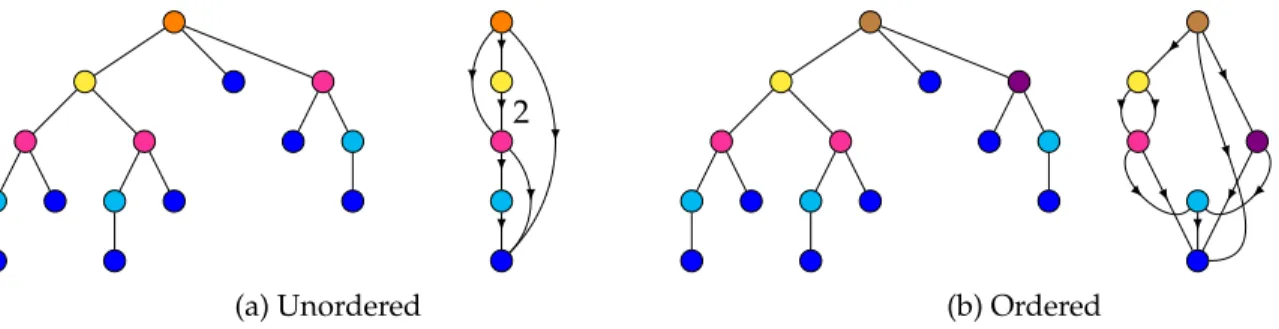
edges. We refer to Fig.3afor an example of DAG reduction of an unordered tree. Two different algorithms that allow the computation of the DAG reduction of an unordered tree but that share the same time-complexity inO(#T2deg(T)log(deg(T)))are presented in [15].

Ordered trees In the case of ordered trees, it is required to preserve the order of the children

in the DAG reduction. As for unordered trees, we consider the quotient graph Q(T) = (V, E)

obtained fromT using the equivalence relation between ordered trees. Vis the set of equivalence classes on the subtrees ofT. Here, the edges of the graph are ordered as follows. (C₁, C₂) is the

rth edge betweenC₁ andC₂if R(C₂) is therth child ofR(C₁) up to an isomorphism. We obtain a DAG with ordered edges that compresses the initial tree T. An example of DAG reduction of an ordered tree is presented in Fig.3b. Polynomial algorithms have been developed to allow the computation of a DAG, with complexities ranging inO(#T2)toO(#T)for ordered trees [12].

2

(a) Unordered (b) Ordered

Figure 3: A tree (left) and its DAG reduction (right) seen (a) as an unordered tree and (b) as an ordered tree. In each figure, roots of isomorphic subtrees are displayed with the same color, which is reproduced on the corresponding vertex of the DAG. Note that the subtree on the left is colored differently in the two cases, whether the order of its children is relevant or not. If no label is specified on an edge (in the unordered case), it is equal to1.

In this paper, R∗(T) denotes the DAG reduction of T as ∗-tree, ∗ ∈ {ordered,unordered}. It is crucial to notice that the function R∗ is a one-to-one correspondence, which means that DAG

(11)

reduction is a lossless compression algorithm. In other words,T can be reconstructed fromR∗(T)

and(R∗)−1_{stands for the inverse function.}

The DAG structure inherits of some properties of trees. For a vertexνin a DAGD, we will denote byC(ν)(P(ν), respectively) the set of children (parents, respectively) ofν. H(ν) and deg(ν) are inherited as well. Similarly to trees, we denote byD[ν]the subDAG rooted in νcomposed ofν

and all its descendants inD. 3.2 DAG reduction of a forest

Let TFT be the super-tree obtained from a forest of∗-treesFT = (T1, . . . , TN) by placing in this

order each Ti as a subtree of an artificial root. We define the DAG reduction of the forestFT as R∗(_FT) = R∗(TFT).

However, if the forestFT is stocked as a forest of compressed DAGs, that is,FD = (D1, . . . , DN)

(withD_i = R∗(T_i)), it would be superfluous to decompress all trees before reducing the super-tree. So, one would rather computeR∗(_FT)directly from FD. From now on, we consider only

forests of DAGs that we will denote unambiguouslyF. In this context,R∗(_F)stands for the DAG reduction of the forest of trees((R∗)−1(D₁), . . . ,(R∗)−1(D_N)). We define the degree of the forest as deg(_F) =maxN

i=1deg(Di).

Computing R∗(_F) from (D₁, . . . , D_N) is in two steps: (i) we construct a super-DAG DF from F = (D₁, . . . , D_N)by placing in this order each D_i as a subDAG of an artificial root (with time-complexityO(deg(_F)PN_i₌₁#D_i)), and (ii) we recompressDF using Algorithm1. Fig.4illustrates

step by step Algorithm1on a forest of two trees seen as unordered then ordered trees.

Proposition 3.1. Algorithm1correctly computesR∗(_F).

Proof. Starting from the leaves, we examine all vertices of same height inDF. Those with same

children (with respect to∗) are merged into a single vertex. The algorithm stops when at some height h, we cannot find any vertices to be merged. Vertices that are merged in the algorithm represents isomorphic subtrees, so it suffices to prove that the algorithm stops at the right time. Lethbe the first height for whichσ(h) =_∅.

Suppose by contradiction that some vertices were to be merged at some height h0 > h. They represents isomorphic subtrees, so that their respective children should also be merged together, and all of their descendants by induction. As any vertex of heighth00+1admits at least one child of heighth00,σ(h)would not be empty, which is absurd. f

Proposition 3.2. Algorithm1has time-complexity:

1. O(#DFdeg(F)(log deg(F) +H(DF)))for unordered trees;

2. O(#DFdeg(F)H(DF))for ordered trees.

Proof.The proof lies in AppendixB. f

Remark 3.3. One might also want to treat online data, but without recompressing the whole dataset when

adding a single entry in the forest. LetR∗(_F)be the already recompressed forest andDa new DAG to be introduced in the data. It suffices to placeDhas the rightmost child of the artificial root ofR∗(_F)to get

(12)

Algorithm 1:DAGRECOMPRESSION

Data:DF the superdag obtained from a forest of DAG reductions of∗-trees,

∗ ∈{ordered,unordered}

Result: R∗(_F)

1 Construct, within one exploration ofDF, the mappingh7→DFh whereDFhis the set of

vertices ofDF at heighth

2 forhfrom0toH(DF) −1do

3 Letσ(h) =f−1({S}) :S∈Imf,#f−1({S})≥2 be the set of vertices to be merged at

heighth, wheref:ν_∈DFh 7→C(ν)

4 ifσ(h) =_∅then

5 Exit algorithm;

6 else

7 forMinσ(h)do

8 Choose one elementνMinMto remain inDF

9 Denote byδM the other elements ofM

10 forνinDF such thatH(ν)> hdo

11 forµinC(ν)such that∃M∈σ(h),δM3µdo

12 DeleteµfromC(ν)

13 AddνMinC(ν)

14 forM∈σ(h)do

15 DeleteδM fromDF

16 returnDF

It should be noticed that Imf(that appears line 3) depends on∗. Indeed, if∗= ordered, Imfis the set of alllistsof

(13)

(a) Figur e 4: An illustration step by step of the Algorithm 1 with ( a ) two tr ees T1 (in cyan ) and T2 (in yellow), seen as ( b ) unor der ed or ( c ) or der ed tr ees. One can observe the DAGs (left) and the execution of the algorithm (right). At each step 1, 2 and 3, we examine vertices at height (0,1,2) and mer ge those which have same childr en. At step 4, we can not find any vertex to mer ge and we stop. Note that in ( c ) at step 3, we find two pairs of vertices to be mer ged : we ar e not restricted to one pair per height. Mer ged vertices ar e color ed in red . The artificial root is color ed in black . 1 2 = 2 2 = 3 2 = 4 2 6 = 2 (b) 1 = 2 = 3 = = 4 6 = (c)

(14)

3.3 DAG annotation and kernel computation

We consider a dataset composed of two parts: the train datasetXtrain= (T1, . . . , Tn)and the dataset

to predictXpred = (Tn+1, . . . , TN). In the train dataset, the classes of the data are assumed to be

known. Our aim is to compute two Gram matricesG= [K(Ti, Tj)]_i,j, where: • (i, j)_{∈ X}_train_{× X}_trainfor the training matrixG_train;

• (i, j)_{∈ X}_pred_{× X}_trainfor the prediction matrixG_pred.

SVM algorithms will useG_train to learn their classifying rule, and G_pred to make predictions [9, Section 6.1]. Other algorithms, such as kernel PCA, would also require to compute a Gram matrix before processing [25, Section 14.2]. We denote by∆ = R∗(_X_train_{∪ X}

pred)the DAG reduction of the dataset and, for any1_≤i_≤N,D_i = R∗(T_i). DAG computation of the subtree kernel requires to annotate the DAG with different pieces of information.

Origins In order to compute the subtree kernel, it will be necessary to retrieve from the vertices

of ∆ their origin in the dataset, that is, from which tree they come from. For any vertex ν in

∆\_R(∆), the origin ofνis defined as

o(ν) =i_∈{1, . . . , n, n+1, . . . , N}:D_i₃ν .

Assuming that(D₁, . . . , D_N)are children of the root of∆in this order (which is achieved if∆had been constructed following the ideas developed in Subsection3.2) leads to the following proposi-tion.

Proposition 3.4. Origins can be calculated using the recursive formula,

∀ν_∈∆\_R(∆), o(ν) =    {i} ifνis theithchild ofR(∆), S p∈P(ν) o(p) otherwise.

Proof. Using the assumption, origins are correct for the children of R(∆). If Di 3 νfor some

i_∈{1, . . . , N}andν_∈∆, thenD_i_{⊇ D}(ν). The statement follows by induction. f

Frequency vectors Remember that in (2)N_τ(T)counts the number of subtrees of a treeT that are

∗-isomorphic to the treeτ. To compute the kernel, we need to know this value, and we claim that we can compute it using only∆. We associate to each vertexν_∈∆\_R(∆)a frequency vectorϕν

where, for any1_≤i_≤N,ϕ_ν(i) =N_(R∗₎−1₍_∆_[_ν_])(T_i).

Proposition 3.5. Frequency vectors can be calculated using the recursive formula,

∀ν_∈∆\_R(∆), ϕν=    (1_{i∈o(ν)})i∈{1,...,N} ifν∈ C(R(∆)), P p∈P(ν) L(p, ν)ϕ_p otherwise,

where either L(p, ν) = 1 if _∗ = ordered, or L(p, v) is the label on the edge betweenp and ν in∆ if

(15)

Proof.Letνbe in∆\_R(∆). Ifν_{∈ C}(_R(∆)), thenνrepresents the root of a treeT_i(possibly several trees if there are repetitions in the dataset), and thereforeϕ_ν(i) =N_T_i(T_i) =1. Otherwise, suppose by induction thatϕp(i)is correct for allp∈ P(ν), and anyi. We fixp∈ P(ν). νappearsL(p, ν)

times as a child ofp, so if(R∗)−1(∆[p])appearsϕ_p(i)times inT_i, then the number of occurrences of(R∗)−1_(∆[ν])_in_T

ias a child of(R∗)−1(∆[p])isL(p, ν)ϕp(i). Summing over allp∈ P(ν)leads

ϕν(i)to be correct as well. f

DAG weighting The last thing that we lack to compute the kernel is the weight function.

Re-member that it is defined for trees as a function w : _T → R+. As we only need to know the weights of the subtrees associated to vertices of∆, we define the weight function for DAG as, for anyν_∈∆,ων =w(R∗₎−1₍_∆_[_ν_]).

Remark 3.6. In light of Propositions3.4and3.5, it should be noted that bothoandϕcan be calculated in

one exploration of∆. By definition, this is also true forω.

DAG computation of the subtree kernel We introduce the matching subtrees functionMas

M:{1, . . . , N}2→2∆

(i, j)₇→{ν_∈∆:{i, j}_⊆o(ν)}

where 2∆ is the powerset of the vertices of∆. Note thatM is symmetric. This leads us to the following proposition.

Proposition 3.7. For anyTi, Tj ∈ X_train∪ X_pred, we have K(T_i, T_j) = X

ν∈M(i,j)

ω_νϕ_ν(i)ϕ_ν(j).

Proof. By construction, it suffices to show thatR∗(_S(Ti)∩ S(Tj)) =M(i, j). Letτ ∈ S(Ti)∩ S(Tj).

Then R∗(τ) _∈ R∗(T_i) and R∗(τ) _∈ R∗(T_j). Necessarily, R∗(τ) _∈ ∆ and {i, j} _⊆ o(R∗(τ)). So

R∗(τ) _{∈ M}(i, j). Reciprocally, letν _{∈ M}(i, j). We denoteτ = (R∗)−1(ν). As{i, j} _⊆ o(ν), then

τ_{∈ S}(T_i)_{∩ S}(T_j). f

Remark 3.8. Mcan be created inO(N2#∆)within one exploration of∆and allows afterward

computa-tions of the subtree kernelK(T_i, T_j)in_O(#M(i, j)) =_O(min(#D_i,#D_j)), which is more efficient than the

O(#T_i+#T_j)algorithm proposed in [30] (the time-complexity is announced in [21, Section 1]). However, since the whole process through Algorithm1is costly, the global method that we propose in this paper is not faster than existing algorithms. Nonetheless, our algorithm is particularly adapted to repeated computa-tions from the same data, e.g., for tuning parameters. Indeed, onceMand∆have been created, they can be stored and are ready to use. An illustration of this property is provided from experimental data in Fig.19.

(16)

Remark 3.9. The DAG computation of the subtree kernel investigated in this section relies on the references [1,10]. Our work and the aforementioned papers are different and complementary. First, our framework is valid for both ordered and unordered trees, while these papers focus only on ordered trees. In addition, the method developed in [1,10] is only adapted to exponential weights (see equations (3.12) and (6.2) from [10]). Thus, even if this algorithm is also based on DAG reduction of trees, it is less general than ours since the weight function is not constrained (see in particular Section4where the weight function is learned from the data). Finally, in [1, Section 4], the time-complexities are studied only from a numerical point of view, while we state theoretical results.

4 Discriminance weight function

For a given probability level and a given classification error, and under the stochastic model of Subsection 2.2, we state in Subsection 2.4 that the sufficient size of the training dataset is min-imum when the weight of leaves is0. In other words, counting the leaves, which are the only subtrees that appear in both classes, does not provide a relevant information to the classification problem associated to this model. As mentioned in Remark 2.5, we conjecture that, in a more general model, this result would be true for any subtree present in both classes. In this section, we propose to rely on this idea by defining a new weight function, learned from the data and called discriminance weight that assigns a large weight to subtrees, that help to discriminate the classes, i.e., that are present or absent in exactly one class, and a low weight otherwise.

The training dataset is divided into two parts:Xweight= (T1, . . . , Tm)to learn the weight function,

andX_class= (Tm+1, . . . , Tn)to estimate the Gram matrix. For the sake of readability,∆denotes the

DAG reduction of the whole dataset, includingXweight,Xclass andXpred. In addition, we assume that the data are divided intoKclasses numbered from1toK.

For any vertexν_∈∆\_R(∆), we define the vectorρνof lengthKas, ∀1_≤k_≤K, ρ_ν(k) = 1

#C_k

X

Ti∈Ck

1_{_i∈o(ν)},

where(C_k)₁≤k≤Kforms a partition ofX_weightsuch thatTi ∈Ckif and only ifTiis in classk. In other

words,ρν(k)is the proportion of data in classkthat contain the subtree(R∗)−1(∆[ν]). Therefore, ρ_ν belongs to the K-dimensional hypercube. It should be noticed thatρ_ν is a vector of zeros as soon as(R∗)−1(∆[ν])is not a subtree of a tree ofX_weight.

For any1 _≤ k _≤ K, lete_k (e_k, respectively) be the vector of zeros with a unique1in positionk

(vector of ones with a unique0in positionk, respectively). If ρ_ν = e_k, the vertexνcorresponds to the subtree(R∗)−1(∆[ν]), which only appears in classk: νis thus a good discriminator of this class. Otherwise, ifρ_ν=e_k, the vertexνappears in all the classes except classkand is still a good discriminator of the class. For any vertexν,δ_ν measures the distance betweenρ_ν and its nearest point of interestekorek,

δ_ν=minK

k=1 min(|ρν−ek|,|ρν−ek|).

It should be noted that the maximum value of δ_ν depends on the number of classes and can be larger than 1. If δν is small, then ρν is close to a point of interest. Consequently, since ν

(17)

weight of a vertexνis defined asω_ν = f(1−δ_ν), wheref : (−∞, 1] → [0, 1]is increasing with

f(x) =0forx_≤0andf(1) =1. Fig.5illustrates some usual choices forf. In the sequel, we chose

ων = f∗(1−δν) with the smoothstep function f∗ :x 7→ 3x2−2x3. We borrowed the smoothstep

function from computer graphics [13, p. 30], where it is mostly used to have smooth transition in a threshold function.

Figure 5: The discriminance weight is defined byω_τ = f(1−δ_τ) where

f: (−∞, 1]→[0, 1]is increasing with

f(0) = 0 andf(1) = 1. This figure presents some usual choices forf.

0 1 1 identity smoothstep smoothstep◦smoothstep threshold

Since leaves appear in all the trees of the training dataset,ρ• is a vector of ones and thusδ• = 1,

which implies ω• = 0. This is consistent with the result developed in Subsection 2.4 on the

stochastic model. As aforementioned, the discriminance weight is inspired from the theoretical results established in Subsection 2.4and the conjecture presented in Remark 2.5. The relevance in practice of this weight function will be investigated in the sequel of the paper through two applications.

Remark 4.1. The discriminance weight is defined from the proportion of data in each class that contain

a given subtree, for all the subtrees appearing in the dataset. It is thus required to enumerate all these subtrees. This is done, without redundancy, via the DAG reduction∆of the dataset defined and investigated in Section 3. As the m trees of the training dataset dedicated to learning the discriminance weight are partitioned intoK classes, computing one ρν vector is of complexityO(m). Therefore, computing all of

them is in_O(#∆m). In addition, computing all values ofδν is in O(#∆K2), as there are2K Euclidean

distances to be computed for each vector of length K. All gathered, computing the discriminance weight function has an overall complexity ofO(#∆(N+K2)).

5 Real data analysis

This section is dedicated to the application of the methodology developed in the paper to eight real datasets with various characteristics in order to show its strengths and weaknesses. The related questions are supervised classification problems. As mentioned in Subsection3.3, our approach consists in computing the Gram matrices of the subtree kernel via DAG reduction and with a new weight function called the discriminance (see Section 4). In particular, we aim to compare the usual exponential weight of the literature and the latter in terms of prediction capability. In all the sequel, the Gram matrices are used as inputs to SVM algorithms in order to tackle these classification problems. We emphasize that this approach is not restricted to SVM but can be applied with other prediction algorithms.

5.1 Preliminaries

In this subsection, we introduce (i) the protocol that we have followed to investigate several datasets, together with a description of (ii) the classification metrics that we use to assess the

(18)

quality of our results, (iii) an extension of DAG reduction to take into account discrete labels on vertices of trees, and (iv) the standard method to convert a markup document into a tree. It should be already noted that all the datasets presented in the sequel are composed of trees (that can be ordered or unordered, labeled or not) together with their class.

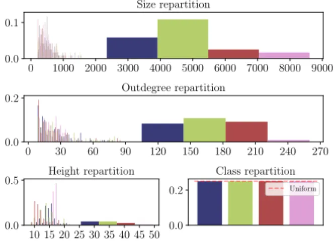
Protocol For each dataset, we have followed the same presentation and procedure. First, a

de-scription of the data is made notably via histograms describing the size, outdegree, height and class repartition of trees. Given the dispersion of some of these quantities, we have binned together the values that does not fit inside the interval [Q₁ − 1.5_·IQR;Q₃ + 1.5_·IQR] where

IQR=Q3−Q1is the interquartile range. Therefore, the flattened-large bins that appears in some

histograms represents those outliers bins. The objective of this part is to show the wide range of datasets considered in the paper.

In a second time, we evaluated the performance of the subtree kernel on a classification task via two methods: (i) for exponential weights τ ₇→ λH(τ) we randomly split the data in half, one for training a SVM, and one for prediction; (ii) for discriminance weight, we randomly split the data in thirds, one for training the discriminance weight, one for training a SVM, and the last one for prediction. We repeated50times this random split for discriminance, and for different values of

λ. The classification results are assessed by some metrics defined in the upcoming paragraph, and gathered in boxplots. The first application example, presented in Subsection5.2, is slightly differ-ent since (i) we have worked with50distinct databases, and (ii) the results have been completed with a deeper analysis of the discriminance weights, in relation with the usual weighting scheme of the literature.

Classification metrics To quantify the quality of a prediction, we use four standard metrics that

are accuracy, precision, recall and F-score. For a class k, one can have true positives TP_k, false positives FP_k, true negatives TN_k and false negatives FN_k. In a binary classification problem, those metrics are defined as,

Accuracy(k) = TPk+TNk TPk+FPk+FNk+TNk , Precision(k) = TPk TP_k+FP_k, Recall(k) = TPk TP_k+FN_k,

F-score(k) = 2Precision(k)Recall(k)

Precision(k) +Recall(k).

For a problem withK > 2classes, we adopt the macro-average approach, that is,

Metric= 1 K K X k=1 Metric(k).

We used the implementation available in thescikit-learnPython library, via the two functions

(19)

DAG reduction with labels In the sequel, some of the presented datasets are composed of la-beled trees, that are trees which each vertex possesses a label. Labels are supposed to take only a finite number of different values. Two labeled ∗-trees are said isomorphic if (i) they are ∗ -isomorphic, and (ii) the underlying one-to-one correspondence mapping vertices ofT₁ into ver-tices ofT₂is such that∀v _∈ T₁,vandΦ(v)have the same label. The set of labeled ∗-trees is the quotient set of rooted trees by this equivalence relation. It should be noticed that the subtree ker-nel as well as DAG reduction are defined through only the concept of isomorphic subtrees. As a consequence, they can be straightforwardly extended to labeled∗-trees. This formalization is an extension of the definition introduced by the authors of [1,10], as they consider only ordered labeled trees, whereas we can consider unordered labeled trees as well.

From a markup document to a tree Some of the datasets come from markup documents (XML

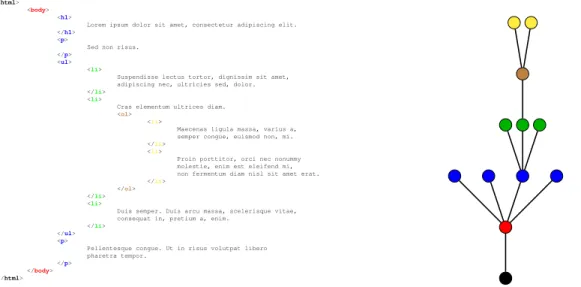
orHTMLfiles). From such a document, one can extract a tree structure, identifying each couple of opening and closing tags as a vertex, which children are the inner tags. It should be noticed that, during this transcription, semantic data is forgotten: the tree only describes the topology of the document. Fig.6illustrates the conversion fromHTMLto tree on a small example. Such a tree is ordered but can be considered as unordered. Finally, a tag can also be chosen as a label for the corresponding vertex in the tree.

<html> <body>

<h1>

Lorem ipsum dolor sit amet, consectetur adipiscing elit. </h1>

<p>

Sed non risus. </p>

Suspendisse lectus tortor, dignissim sit amet, adipiscing nec, ultricies sed, dolor. </li>

<li>

Cras elementum ultrices diam. <ol>

<li>

Maecenas ligula massa, varius a, semper congue, euismod non, mi. </li>

<li>

Proin porttitor, orci nec nonummy molestie, enim est eleifend mi, non fermentum diam nisl sit amet erat. </li>

</ol> </li> <li>

Duis semper. Duis arcu massa, scelerisque vitae, consequat in, pretium a, enim.

</li> </ul> <p>

Pellentesque congue. Ut in risus volutpat libero pharetra tempor.

</p> </body> </html>

Figure 6: Underlying ordered tree structure (right) present in aHTMLdocument (left). Each level in the tree is colored in the same way as the corresponding tags in the document. Natural order from top to bottom in theHTMLdocument corresponds to left-to-right order in the tree.

5.2 Prediction of the language of a Wikipedia article from its topology

Classification problem and results Wikipedia pages are encoded in HTML and, as

aforemen-tioned, can therefore be converted into trees. In this context, we are interested in the following question: does the (ordered or unordered) topology of a Wikipedia article (as an HTML page) contain the information of the language in which it has been written? This can be formulated as a supervised classification problem: given a training dataset composed of the tree structures

(20)

of Wikipedia articles labeled with their language, is a prediction algorithm able to predict the language of a new data only from its topology? The interest of this question is discussed in Re-mark5.1.

In order to tackle this problem, we have built 50 databases of 480 trees each, converted from Wikipedia articles as follows. Each of the databases is composed of4datasets:

• a dataset to predictXpredmade of120trees;

• a small train datasetXsmall

train made of40trees;

• a medium train datasetXmedium

train made of120trees;

• and a large train datasetXtrainlarge made of200trees.

For each dataset, and each language, we picked Wikipedia articles at random using the Wikipedia API1, and converted them into unlabeled trees. It should be noted that the probability to have the same article in at least two different languages is extremely low. For each database, we aim at predicting the language of the trees inXpredusing a SVM algorithm based on the subtree kernel for ordered and unordered trees, and trained withXsize

train where size ∈ {small,medium,large}. Fig.8 provides the description of one typical database. All trees seem to share common characteristics, regardless of their class.

0 1000 2000 3000 4000 5000 6000 7000 8000 9000 0.0 0.1 Size repartition 0 30 60 90 120 150 180 210 240 270 0.0 0.2 Outdegree repartition 10 15 20 25 30 35 40 45 50 0.0 0.5 Height repartition 0.0 0.2 Class repartition Uniform

Figure 7: Description of a Wikipedia dataset (480 trees).

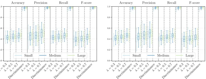
Classification results over the50databases are displayed in Fig.8. Discriminance weighting achie-ves highly better results than exponential weighting, with all metrics greater than90% on average from only200training data. This points out that the language information exists in the structure of Wikipedia pages, whether they are considered as ordered or unordered trees, unlike what in-tuition as well as subtree kernel with exponential weighting suggest. It should be added that the variance of all metrics seem to decrease with the size of the training dataset when using discrimi-nance.

(21)

λ= 0.3 λ= 0.5 λ= 0.7 Discriminance λ= 0.3 λ= 0.5 λ= 0.7 Discriminance λ= 0.3 λ= 0.5 λ= 0.7 Discriminance λ= 0.3 λ= 0.5 λ= 0.7 Discriminance 0.0 0.2 0.4 0.6 0.8 1.0

Accuracy Precision Recall F-score

Small Medium Large

Figure 8: Classification results for the 50 Wikipedia databases as ordered (left) and unordered (right) trees.λvalues stands for exponential decay weight of the formτ₇→λH(τ). The colors of the boxplot indicates, for each size∈{small,medium,large}, the results obtained for the classification ofXpredfromXtrainsize.

These numerical results show the great interest of the discriminance weight, in particular with respect to an exponential weight decay. Nevertheless, it should be compelling in this context to understand the classification rule learned by the algorithm. Indeed, this could lead to explain how the information of the language is present in the topology of the article.

Comprehensive learning and data visualization When a learning algorithm is efficient for a

given prediction problem, it is interesting to understand which features are significant. In the subtree kernel, the features are the subtrees appearing in all the trees of all the classes. Looking at (2), the contribution of any subtreeτto the subtree kernel with discriminance weighting is the product of two terms: the discriminance weightwτ quantifies the ability of τ to discriminate a

class, whileκ(N_τ(T₁), N_τ(T₂))evaluates the similarity betweenT₁andT₂with respect toτthrough the kernelκ. As explained in Section4, ifwτis close to1,τis an important feature in the prediction

problem.

As shown in Section 3, DAG reduction provides a tool to compress a dataset without loss. We recall that each vertex of the DAG represents a subtree appearing in the data. Consequently, we propose to visualize the important features on the DAG of the dataset where the radius of the vertices is an increasing function of the discriminance weight. In addition, each vertex of the DAG can be colored as the class that it helps to discrimine, either positively (the vertex of the DAG corresponds to a subtree that is present almost only in the trees of this class), or negatively. This provides a visualization at a glance of the whole dataset that highlights the significant features for the underlying classification problem. We refer the reader to Fig.9for an application to one of our datasets. Thanks to this tool, we have remarked that the subtree corresponding to the License at the bottom of any article highly depends on the language, and thus helps to predict the class.

(22)

en: absence en: pr esence es: absence es: pr esence de: absence de: pr esence fr: absence fr: pr esence Figur e 9: V isualization of one dataset X = X medium train ∪ Xpr ed of unor der ed tr ees among the 30 W ikipedia databases. Each vertex ν ∈ R ∗ (X ) is scaled accor ding to f ∗ ( 1 − δν ) so that the lar gest vertices ar e those that best discriminate the dif fer ent classes. For each ν , we find the class k such that ρν has minimal distance to either ek or ek . If it is ek , we say that ν discriminates by its pr esence, and if it is ek , ν discriminates by its absence. W e color ν following this distinction accor ding to the legend, wher e “en” is for English language, “de” for German, “fr ” for Fr ench, and “es” for Spanish.

(23)

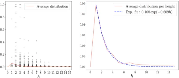
Distribution of discriminance weights To provide a better understanding of our results, we have analyzed in Fig.10 the distribution of discriminance weights of one of our large training datasets. It shows that the discriminance weight behaves on average as a shifted exponential. Considering the great performance achieved by the discriminance weight, this illustrates that ex-ponential weighting presented in the literature is indeed a good idea, when setting w• = 0 as

shown in Subsection 2.4or suggested in [30, 6 Experimental results]. However, a closer look to the distribution in Fig.10(left) reveals that important features in the kernel are actually outliers: relevant information is both far from the average behavior and scarce. To a certain extent and regarding these results, discriminance weight is the second order of the exponential weight.

Figure 10: Estimation of the distribution of the discriminance weight functionh₇→ {w_ν :_H(ν) = h, ν _∈ R∗(_X)}from one large training Wikipedia dataset of unordered trees (left) and fit of its average behavior (inred) to an exponential function (inblue). All ordered and unordered datasets show a similar behavior.

Remark 5.1. The classification problem considered in this subsection may seem unrealistic as ignoring the

text information is obviously counterproductive in the prediction of the language of an article. Neverthe-less, this application example is of interest for two main reasons. First, this prediction problem is difficult as shown by the bad results obtained from the subtree kernel with exponential weights (see Fig.8). As high-lighted in Fig.9and10(left), the subtrees that can discriminate the classes are very unfrequent and diverse (in terms of size and structure), so difficult to be identified. On a different level, as Wikipedia has a very large corpus of pages, it provides a practical tool to test our algorithms and investigate the properties of our approach. Indeed, we can virtually create as many different datasets as we want by randomly picking articles, ensuring that we avoid overfitting.

5.3 Markup documents datasets

We present and analyze in this subsection three datasets obtained from markup documents.

INEX 2005 and 2006 These datasets originate from the INEX competition [11]. There are XML

(24)

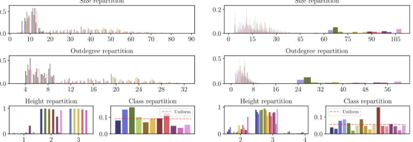
2005 is made of 9 630 documents arranged in 11 classes, whereas INEX 2006 has 18 classes for 12 107 documents. For INEX 2005, classes can be split into two groups of trees with similar char-acteristics, as shown in Fig.11(left). However, inside each group, all trees are alike. In the case of INEX 2006, no special group seems to emerge from topological characteristics of the data, as pointed out in Fig.11(right).

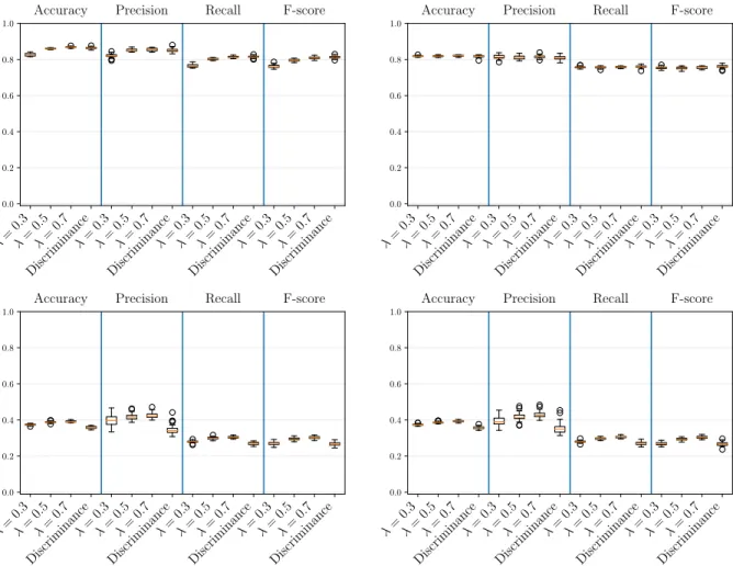
The classification results are depicted in Fig.12, for both datasets, and with trees considered suc-cessively as ordered and unordered. For INEX 2005, both exponential decay and discriminance achieve similar good performance. However, for INEX 2006, neither of them are able to achieve significant results. Actually, discriminance performs slightly worse than exponential decay. From these results we deduce that subtrees do not seem to form the appropriate substructure to capture the information needed to properly classify the data.

0 10 20 30 40 50 60 70 80 90 0.0 0.5 Size repartition 4 8 12 16 20 24 28 32 0.0 0.5 Outdegree repartition 1 2 3 0 1 Height repartition 0.0 0.1 Class repartition Uniform 0 15 30 45 60 75 90 105 0.0 0.2 Size repartition 0 8 16 24 32 40 48 56 0.0 0.5 Outdegree repartition 2 3 4 0 1 Height repartition 0.0 0.1 Class repartition Uniform

Figure 11: Description of INEX 2005 (9 630 trees, left) and INEX 2006 (12 107 trees, right) datasets.

Videogame sellers We manually collected, for two major websites selling videogames2, the

URLs of the top 100 best-selling games, and converted them into ordered labeled trees. As web-pages might seem similar to some extent, the trees are actually very different, as highlighted in Fig.13. We found that the subtree kernel retrieves this information as, for both exponential decay and discriminance weights, we achieved 100% of correct classifications in all our tests.

5.4 Biological datasets

In this subsection, three datasets from the literature are analyzed, all related to biological topics.

Vascusynth The Vascusynth dataset from [16,20] is composed of 120 unordered trees that

rep-resent blood vasculatures with different bifurcations numbers. In a tree, each vertex has a contin-uous label describing the radiusrof the corresponding vessel. We have discretized these contin-uous labels in three categories: small ifr < 0.02, medium if0.02 _≤r < 0.04and large ifr _≥0.04

(all values are in arbitrary unit). We split up the trees into three classes, based on their bifurcation number. Based on Fig.14(left), we can distinguish between the three classes by looking only at

(25)

Figure 12: Classification results for INEX 2005 (top) and INEX 2006 (bottom) as ordered (left) and unordered (right) trees.

the size of trees. Contrary to the videogame sellers dataset that had the same property, the clas-sification does not achieve 100% of good clasclas-sification, as depicted in Fig.14(right). On average, discriminance performs better than the other weights, despite having a larger variance. This is probably due to the small size of the dataset, as the discriminance is learned only with around13

trees per class.

Hicks et al. cell lineage trees Across cellular division, tracking the lineage of a single cell

nat-urally defines a tree. In a recent article, Hicks et al. have been investigating the variability inside cell lineages trees of three different species [19]. From the encoding of the data that they have pro-vided as a supplementary material3, we have extracted ordered unlabeled trees that are presented in Fig.15(left). The dataset contains, for two classes, trees of outdegree 0 (i.e., isolated leaves) that can be considered as noise. With respect to the exponential weight, the value of the kernel between such trees will be identical, whether they belong to the same class or to two different classes. They therefore contribute to reducing the kernel’s ability to effectively discriminate between these two

(26)

400 800 1200 1600 2000 2400 2800 3200 3600 4000 0.00 0.25 Size repartition 15 30 45 60 75 90 105 0.0 0.5 Outdegree repartition 0 150 450 900 0.0 0.2 Height repartition 0.0

0.5 Class repartition_Uniform

Figure 13: Description of the videogame sellers dataset (200 trees).

0 15 30 45 60 75 90 105 120 0.0 0.5 Size repartition 2 0 1 Outdegree repartition 3 6 9 12 15 18 21 24 0.00 0.25 Height repartition 0.0 0.2 Class repartition Uniform λ= 0.3 λ= 0.5 λ= 0.7 Discriminance λ= 0.3 λ= 0.5 λ= 0.7 Discriminance λ= 0.3 λ= 0.5 λ= 0.7 Discriminance λ= 0.3 λ= 0.5 λ= 0.7 Discriminance 0.0 0.2 0.4 0.6 0.8 1.0

Figure 14: Description of the Vascusynth dataset (120 trees, left) and classification results (right).

classes. On the other hand, the discriminance weight will assign them a zero value, “de-noising”, in a way, the data. This observation may explain why discriminance weight achieves better results than exponential weight.

Faure et al. cell lineage trees Faure et al. have developed a method to construct cell lineage trees

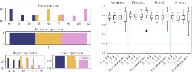
from microscopy [14] and provided their data online4. We extracted 300 unordered and unlabeled trees, divided between three classes. It seems from Fig.16 (left) that one class among the three can be distinguished from the two others. Classification results can be found in Fig.16 (right): the discriminance weight performs better than the exponential weight, whatever the value of the parameter.

4_{https://bioemergences.eu/bioemergences/openworkflow-datasets.php} _{(last accessed in October}

(27)

0 60 120 180 240 300 360 420 480 540 0.0 0.5 Size repartition 0 1 2 0 1 Outdegree repartition 0 2 4 6 8 0.0 0.5 Height repartition 0.0 0.5 Class repartition Uniform λ= 0.3 λ= 0.5 λ= 0.7 Discriminance λ= 0.3 λ= 0.5 λ= 0.7 Discriminance λ= 0.3 λ= 0.5 λ= 0.7 Discriminance λ= 0.3 λ= 0.5 λ= 0.7 Discriminance 0.0 0.2 0.4 0.6 0.8 1.0

Figure 15: Description of the Hicks et al. dataset (345 trees, left) and classification results (right).

32 40 48 56 64 72 80 88 0.0 0.5 Size repartition 1 2 3 0 1 Outdegree repartition 26 27 28 29 30 0 1 Height repartition 0.0 0.2 Class repartition Uniform λ= 0.3 λ= 0.5 λ= 0.7 Discriminance λ= 0.3 λ= 0.5 λ= 0.7 Discriminance λ= 0.3 λ= 0.5 λ= 0.7 Discriminance λ= 0.3 λ= 0.5 λ= 0.7 Discriminance 0.0 0.2 0.4 0.6 0.8 1.0

Figure 16: Description of the Faure et al. dataset (300 trees, left) and classification results (right). 5.5 LOGML

The LOGML dataset is made of user sessions on an academic website, namely the Rensselaer Polytechnic Institute Computer Science Department website5, that registered the navigation of users across the website. 23 111 unordered labeled trees are present, divided into two classes. The trees are very alike, as shown in Fig.17(left), and the classification results of Fig.17(right) are very similar to INEX 2005, where all weight functions behave similarly, without any advantage for the discriminance weight in terms of prediction.

(28)

0 40 80 120 160 200 240 280 0.0 0.2 Size repartition 0 15 30 45 60 75 90 105 120 0.00 0.25 Outdegree repartition 0 15 30 45 60 75 90 105 0.00 0.25 Height repartition 0.0 0.5 Class repartition Uniform λ= 0.3 λ= 0.5 λ= 0.7 Discriminance λ= 0.3 λ= 0.5 λ= 0.7 Discriminance λ= 0.3 λ= 0.5 λ= 0.7 Discriminance λ= 0.3 λ= 0.5 λ= 0.7 Discriminance 0.0 0.2 0.4 0.6 0.8 1.0

Figure 17: Description of the LOGML dataset (23 111 trees, left) and classification results (right).

6 Concluding remarks

6.1 Main interest of the DAG approach: learning the weight function

In Section 2, we have shown on a 2-classes stochastic model that the efficiency of the subtree kernel is improved by imposing that the weight of leaves is null. As explained in Remark2.5, we conjecture that the weight of any subtree present in two different classes should be0. The main interest of the DAG approach developed in Section3is that it allows to learn the weight function from the data, as developed in Section4with the discriminance weight function. Our method has been implemented and tested in Section5on eight real datasets with very different characteristics that are summed up in Table1.

As a conclusion of our experiments, we have analyzed the relative improvement in prediction obtained with the discriminance weight against the best exponential weight in order to show both the importance of the weight function and the relevance of the method developed in this paper. More precisely, for each dataset and each classification metric, we have calculated

RI= Metricdiscr−max(Metricλ)

max(Metricλ)

,

from the average values of the different metrics. The results are presented in Fig.18. We have found that, except in one case, discriminance behaves as good as exponential weight decay and even performs better in most of the datasets. Furthermore, one can observe a kind of trend, where the relative improvement decreases when the number of trees in the training dataset is increasing, which proves the great interest of the discriminance to handle small datasets, provided that (i) the problem is difficult enough that the exponential weights are not already high performing, as it is the case in the Videogames sellers dataset, and (ii) the dataset is not too small, as for Vascusynth. Indeed, as the discriminance is learned independently from the SVM, one must have enough training data to divide them efficiently. Nevertheless, it should be noted that, in the framework of the DAG approach, results from the discriminance weight can be obtained much faster due to the fact that the Gram matrices are estimated from one half of the training dataset, while learning

(29)

the discrimance is very fast as it can be done in one traversal of the DAG (see time-complexity presented in Remark4.1). Finally, we have investigated on a single example some properties of the discriminance, discovering that it can be interpreted as a second-order exponential weight, as well as a method for visualizing the important features in the data.

Dataset WikipediaVideogamesINEX 2005 INEX 2006 VascusynthHicks etal. Faur e etal. LOGML Ord. / Unord. Both Ord. Both Both Unord. Ord. Unord. Unord.

labeled 7 X X X X 7 7 X

Number of trees 160 – 320 200 9 630 12 107 120 345 300 23 111

Number of classes 4 2 11 18 3 3 3 2

Table 1: Summary of the 8 datasets.

Vascusyn

th

Wikip

edia

- small

Videogame

sellers

Wikip

edia

- medium

Faure

et

al.

Wikip

edia

- large

Hic

ks

et

al.

INEX

2005

INEX

2006

LOGML

−20 0 20 40 60 80 100 120 140

Accuracy

Precision

Recall

F-score

Figure 18: Relative improvementRI(in percentage) of the discriminance against the best value of

λfor all datasets (sorted by increasing number of trees in the training dataset) and all metrics.

6.2 Interest of the DAG approach in terms of computation time

As shown in Fig.16(right), the exponential decay classification results for the Faure et al. dataset are very dependent on the value chosen for the parameterλ. In this case, it can be interesting to tune this parameter and estimate its best value with respect to a prediction score. This requires to