A One-Class Support Vector Machine Calibration Method for Time Series Change Point Detection

A One-Class Support Vector Machine Calibration Method for Time

Series Change Point Detection

Baihong Jin

Yuxin Chen

Dan Li

Kameshwar Poolla

Alberto Sangiovanni-Vincentelli

_{Department of EECS, University of California, Berkeley}

{bjin,poolla,alberto}@eecs.berkeley.edu 2

_{California Institute of Technology}

[email protected]

3

_{Institute of Data Science, National University of Singapore}

Abstract—It is important to identify the change point of a system’s health status, which usually signifies an incipient fault under development. The One-Class Support Vector Machine (OC-SVM) is a popular machine learning model for anomaly detection and hence could be used for identifying change points; however, it is sometimes difficult to obtain a good OC-SVM model that can be used on sensor measurement time series to identify the change points in system health status. In this paper, we propose a novel approach for calibrating OC-SVM models. The approach uses a heuristic search method to find a good set of input data and hyperparameters that yield a well-performing model. Our results on the C-MAPSS dataset demonstrate that OC-SVM can also achieve satisfactory accuracy in detecting change point in time series with fewer training data, compared to state-of-the-art deep learning approaches. In our case study, the OC-SVM calibrated by the proposed model is shown to be useful especially in scenarios with limited amount of training data.

Index Terms—Support vector machine, change point detection

I. INTRODUCTION

In system health monitoring, it is important to identify the change point, which usually signifies an incipient fault under development [1]. Change point detection aims to find out when a system starts to shift away from its normal health condition into a faulty state. From a preventive maintenance perspective, it indicates that a maintenance action should be taken soon to intervene the degradation process in order to avoid further damage [2]. Although system degradation is a gradual and complicated process, its development can in general be segmented into four discrete stages [3]: 1) normal degradation, 2) transition region, 3) accelerated degradation, and 4) failure; see Fig. 1 for a detailed illustration. We are interested in locating the transition region, a.k.a. the “knee” of the trajectory of the degrading health index.

In practice, change point detection is often a challenging task, especially in Cyber-Physical System (CPS) applications. As pointed out by authors of [4], conventional change point detection models are often based on strong prior assumptions about the generative process that produces the observed data; however, the assumptions may not hold true for actual systems,

which results in unsatisfactory performance of such methods. As another approach to tackle this challenge, various learning-based approaches have also been employed to distinguish different states in time series data. These approaches can be generally classified intosupervised andunsupervised learning methods. In supervised learning, each data point is associated with a label that tells the category the point belongs to. Based on the supervisory information, a supervised learning algorithm infers a decision function that can be used to assign labels to data points; ideally, the learned decision function can generalize well to unseen new data points. In the Fault Detection and Diagnosis (FDD) literature, supervised methods have been shown to be effective at distinguishing healthy and faulty states, when labels for training data are available. In fact, in real applications it is very difficult to obtain labels that accurately indicate the change point locations of training data, making it a challenge to apply supervised methods for change point detection. Even if we have detected the existence of faults, we do not know when the fault starts to develop. Unsupervised approaches, e.g. One-Class Support Vector Machine (OC-SVM) [5] and autoencoders [6], are more suitable in such scenarios where there are not enough labeled data for differentiating a system’s health status. Still, in OC-SVM and autoencoder approaches, we need to provide a training dataset that comprise of mostly fault-free data. In addition, the choice of hyperparameter may also greatly impact the model’s performance. Without labeled data for cross-validation, it is a challenging task to select the input data and the hyperparameters.

In this paper, we address these challenges by proposing a heuristic approach forcalibratingOC-SVM models. During the calibration, besides the hyperparameters, we also controlled how much training data is used for training the OC-SVM model. The calibrated OC-SVM model is used for detecting the change points in timeseries data. In particular, we study scenarios where: 1) the system can be assumed to be healthy from the start of until a point where faults start to develop, and ends up in a fault state, 2) the degradation can be viewed as an approximately monotonic process. We believe that such setup is representative of many real-world degradation processes. To validate our proposed approach, we conducted a case study on 978-1-5386-8357-6/19/$31.00 ©2019 IEEE

Normal Degradation Transition Accelerated Degradation Failure Time H ea lth In d ex

Fig. 1: The four stages in a typical degradation process [3].

the C-MAPSS dataset [7], and demonstrated strong empirical performance in detecting change points.

The remainder of this paper is organized as follows. In Sec. II, we give necessary background on OC-SVM. Next in Sec. III, we discuss on our proposed search framework in details. A brief description about the C-MAPSS flight engine dataset is provided in Sec. IV, and experimental results is presented in Sec. V. We conclude the paper in Sec. VI and discuss future directions.

II. ONE-CLASSSUPPORTVECTORMACHINE A one-class SVM (OC-SVM) [5] model denotes an unsuper-vised machine learning model that learns a decision function for estimating the support of a dataset. This property makes it applicable to outlier detection. In literature, it has been applied to areas such as fault detection, intrusion detection, and forgery signature detection [8]. An OC-SVM model is trained on data mostly from one class (usually the “normal” class). The trained model can be used to classify new data as similar or different to the training set. This is useful for outlier detection because there are usually very few examples for outliers (anomalies or faults), which makes it difficult to train a two-class classifier to distinguish them.

To obtain more versatile decision boundaries with OC-SVM, kernel functions are often used to map the original feature space into higher-dimensional spaces. Let Φ :X → Z be a mapping from the original data space to a higher-dimensional feature space. To train an OC-SVM model, we solve the following quadratic program. min w,ξi,b 1 2kwk 2 2+ 1 νm m X i=1 ξi−b (1) s.t. ∀i= 1,2, . . . , N ν∈(0,1], ξi≥0, w·Φ(zi)≥b−ξi.

Whereξi is a slack variable for data pointi.ν takes a value

between 0 and 1; it upper bounds the fraction of training errors and lower bounds the fraction of support vectors. As a result, a non-zero ν will allow an OC-SVM model to exclude some of the training data as outliers from the normal class. We use

the following decision function, to decide whether or not an inputxbelongs to the normal class.

f(z) =sign(w·Φ(x)−b) =

(

+1normal,

−1 outlier. (2) In this study, we choose Radial Basis Function (RBF) kernels in our OC-SVM formulation because they do not assume any parametric form of the data distribution, and thus they are suitable for capturing data of complex shape. A RBF kernel has a formK(zi, zj) = exp −γkzi−zjk2, whereγcontrols

the width of the RBF kernel used for training. The largerγ is, the smaller the width of the kernel. If gamma is too large, the model will overfit the data and will not capture the shape of the data distribution.

III. HEURISTICOC-SVM CALIBRATIONAPPROACH Both the input training data and the choice of OC-SVM hyperparameters can influence the prediction performance of OC-SVM models. The choice of the two hyperparametersν and γ can greatly affect the prediction performance of the model. In fact, these hyperparameters are coupled, because ν regulates the percentage of outliers in the training data. If we choose a small ν, then we must ensure that 1−ν of the training data are from the positive class. We are facing a dilemma here: to obtain a good OC-SVM model for change point detection, we must ensure that the training data contains few outliers, which requires us to know the location of the change points a priori. To resolve the dilemma, we resort to a heuristic scheme to search for a suitable assignment of input data and hyperparameters as our hypothesis, such that the predictive outcome matches the hypothesis itself. Since the training of OC-SVM is achieved by solving a quadratic optimization problem, it can be done efficiently with state-of-the-art optimization tools. The fast training time of OC-SVM enables us to use a heuristic optimization approach to search for an optimal configuration, which will be introduced next.

Let us index the m system instances under study by

1,2, . . . , m. By assumption, the systems all degrade in an approximately monotonic fashion. We designate their respective change points by a vectorρ= (ρ1, ρ2, . . . , ρm), where each

ρi∈(0,1)is a number representing the portion of life span

when theith system hits its change point. For example,ρi= 0.7

means that engine i is healthy in the first 70% of its life span before reaching the change point. By fixing ν to a small positive value, we look for an assignment of ρ where the input data are mostly healthy (from the positive class). The decision variable(γ,ρ)now consists of m+ 1 dimensions. A sensible hypothesis of (γ,ρ) will yield an OC-SVM model whose prediction will agree with the hypothesis. We use a Differential Evolution (DE)-based heuristic search scheme to find(γ,ρ). For guiding the heuristic search, a loss function is needed to evaluate thegoodness of fit of each hypothesized hyperparameters. Analogous to hypothesis testing in statistics, if a hypothesis(γ,ρ)does not yield a prediction that isconsistent with itself, we can claim that the hypothesis is probably not true.

A. Loss Function for Examining the “Goodness of Fit” of a Hypothesis

In our scenario, each hypothesizedρisignifies the position of

change point (as a percentage value) of training system instance i. Let the actual position (in cycles) of the change point be ci. In other words, the firstci cycles can be assumed healthy

(labeled 1), while the rest are assumed unhealthy (labeled

0). For each hypothesis(γ,ρ), we will check how consistent it is with the learned OC-SVM classifier and its associated classification results by using the loss function as described below.

L(γ,ρ) =

m X

i=1

log_lossy(i),z(i), (3)

wherey(i)_{is the hypothesized label assignment with the first}

ci elements being1’s, and otherwise0’s.z(i) is the predicted

label assignment from the trained classifier.

When a trained classifier is applied to an unseen system instance, its change point can be derived by finding the point in life that gives the lowest cross-entropy loss (i.e., log loss). B. Differential Evolution for Hyperparameter Optimization

DE is an evolutionary algorithm that is commonly used for solving global optimization problems. The DE optimizes a problem by maintaining a population of candidate solutions and creating new candidate solutions by combining existing ones according to some simple formulae. Candidate solutions that receive better scores are kept and will be used for generating new candidate solutions during the next generation. The optimization problem is thus treated as a black box, and the DE procedure does need gradient information to optimize it. With the loss function described above, we can use DE to search for a hypothesis whose prediction result is consistent with the hypothesized hyperparameter assignment itself. It is worthy to note that there does not need to be an “accurate” optimum, because the change point actually is an interval instead of a single point. Our purpose is achieved, as long as the found change point falls within the transition region.

In this work, we use DE [9], [10] as our search framework. It is worthy to note that, besides DE, other heuristic search algorithms such as Bayesian optimization [11], [12] and simulated annealing [13] may also be applied here. It is part of our ongoing work to test out the effectiveness of these other search algorithms.

IV. C-MAPSS DATASET A. Organization of the C-MAPSS Dataset

The C-MAPSS dataset [7] was originally released in the PHM-08 Challenge. The dataset was generated by a high-fidelity engine simulator. During the simulation for each engine, some fault was injected at a given time and persisted throughout the remaining flights. The degradation process over the lifespan of an engine is described as a multivariate timeseries consisting of a few hundred data points (cycles). Each data point is a 21-dimension vector corresponding to 21 sensor readings. Because

little system-specific knowledge about the engines was given, useful information needs to be mined from data themselves, making the learning problem a data-driven task. Since each timeseries describes the run-to-failure process of an engine, we also know the Remaining Useful Life (RUL) of the engine at each time instant.

The original goal of the PHM-08 Challenge was to stimulate the development of data-driven RUL estimation methods. Since the release of the C-MAPSS dataset, many different RUL estimation approaches are seen in literature. A comprehensive review of the published results can be found in [3]. The dataset consists of four parts (FD001-FD004) that represent an increasing level of complexity.FD001-FD003can be seen as special cases of FD004. The FD001 data represent the simplest scenario, where the engines are operating only at sea level, and are injected with only one type of fault. The

FD004data involves two fault types and six flight conditions. The review paper [3] noticed that many publications used only

FD001, the most basic scenario, for validating their algorithms; their actual performance on more realistic scenarios such as

FD004is thus doubtful. Because of this, theFD004data are used to validate our approach in the experiment.

Given the ground truth RUL number at each observed data point, the RUL prediction problem can be formulated as a regression problem. Supervised learning methods, such as neural networks, can be used to establish a mapping between feature vectors and RUL. Due to their ability to capture complex temporal relationship among data, a number of papers [14], [15] employed variants of Recurrent Neural Network (RNN) to model the functional mapping and reported to yield satisfactory results.

B. Change Point Detection with WTTE-RNN

An accurate RUL regression model, however, does not directly serve our purpose of change point identification. Recently, Martinsson proposed a novel RNN architecture called WTTE-RNN1 _{[16] that provided additional insight into} 1_{The name WTTE-RNN stands for “Weibull Time To Event Recurrent}

Neural Network”.

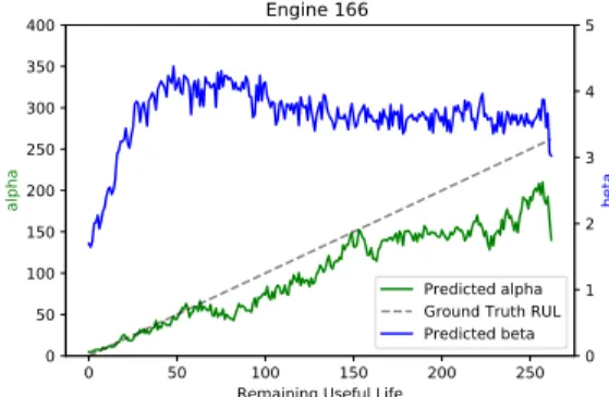
0 50 100 150 200 250

Remaining Useful Life 0 50 100 150 200 250 300 350 400 alpha Engine 166 Predicted alpha Ground Truth RUL Predicted beta 0 1 2 3 4 5 beta

Fig. 2:We implemented and trained a WTTE-RNN model in Keras, using all249engines fromFD004. Trends of predictedαandβon engine instance 166.

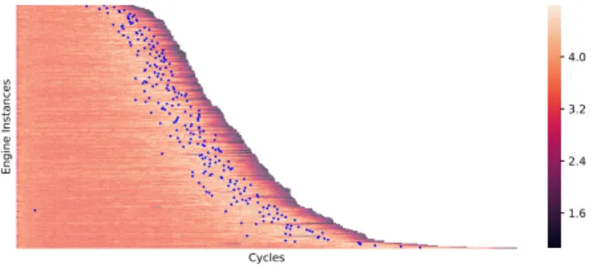
Cycles Engine Instances 1.6 2.4 3.2 4.0 (a) (b)

Fig. 3:(a) The predictedβvalues on all 249 engine instances using our approach (b) The βvalues predicted by another WTTE-RNN model that is trained using only 20 engine instances for comparison purposes. The βvalues are signified by different colors.

the degradation process. Not only can WTTE-RNN provide uncertainty estimation about the predicted RUL, but it also indicates potential changes in the health status. Since the C-MAPSS dataset itself does not provide ground truth information about the change point location for each engine, so we need another approach for validating our proposed approach. In this study, we used the segmentation results given by the WTTE-RNN as the ground truth to benchmark our proposed OC-SVM approach.

Here we brief describe the RNN approach. WTTE-RNN is a WTTE-RNN architecture for time-to-event prediction. As with other RNN architectures, a WTTE-RNN model makes prediction at each time step based on previous input sequences. Specifically, at each time stept, the model predicts two numbers αt andβt, the two parameters of a Weibull distribution that

characterize the RUL at time t. The predicted αt parameter

represents the expected RUL value at time step t, and βt

quantifies the associated uncertainty of the RUL prediction. By feeding the observed timeseries data into the trained WTTE-RNN network, we will obtain sequences of predicted αand β values, which reflect the updating prediction on the system health status.

To illustrate the performance of WTTE-RNN on the C-MAPSS dataset, we implemented a WTTE-RNN model in Keras, and trained the network using all 249 engines from

FD004. As an example, Fig. 2 plots the produced αand β evaluations for engine 166. It can be seen that the producedαt

is able to predict the RUL with good accuracy, especially when the engine is close to its End of Life (EoL). In addition, the β values are large when the engine is healthy, and decreases rapidly when the engine moves towards the EoL. Intuitively, it is usually difficult to predict RUL accurately when an engine is healthy, resulting in relatively high β values, and easier to predict RUL when an engine moves towards its EoL. In particular, we can also observe a short period of increase in β value before it rapidly drops, which indicates higher uncertainties values in this region. We show the predicted β value on all 249 engines as a heatmap in Fig. 3a. It can be seen that the phenomenon mentioned above appears in almost all the engines. Martinsson conjectured [16] that the elevated uncertainty values are due to the transition from the healthy

state to a fast degradation phase, i.e. the “knee” in Fig. 1. More details about the WTTE-RNN approach are beyond the scope of this paper, and we refer interested readers to [16] for a more in-depth discussion.

Although WTTE-RNN has demonstrated promising results, the model when trained with data from only 20 engines fails to give satisfactory results. The resulting β predictions, as displayed in Fig. 3b, do not clearly indicate the change points. This suggests that the performance of this approach might be affected when training data are limited. It will be shown shortly, our approach in comparison requires much fewer data, making it advantageous when the available amount of data is limited.

V. EXPERIMENTALRESULTS

We randomly selectedm= 20out of a total of249engines as the training set, and used the rest as the test set. In our experiment, the population consisted of105individuals, and was evolved for 10 generations. We fixed ν = 0.05 during the heuristic search to reduce the complexity. To further reduce the search space, we assumed the first 50% of the observed data for each training engine is healthy, i.e.∀i, 0.5≤

ρi ≤ 1.0. Because a good value for γ could vary much

(typical values between 10−2 and102), in our DE procedure we search for log10γ ∈ [−2,2] instead. We implement the

algorithm in Python using theOneClassSVMmodule from

scikit-learn for training OC-SVM classifiers, and the

differential_evolution module fromscipy as the

framework for implementing the DE search procedure. After evolving for 10 generations, the DE search procedure returned the optimal OC-SVM model configuration withγ= 3.59, as well as the change point locations for the 20 engines in the training set. To obtain the change point of the rest of the engines, we used the method mentioned in Sec. III. The identified change points by our approach are plotted as the blue points in Fig. 4. As can be seen, for most of the engines, the change points identified by our algorithm match the transition region (white regions with high β values) given by WTTE-RNN. Although the OC-SVM model lacks the ability to predict the RUL, it still identifies the correct change point locations. As opposed to the WTTE-RNN that needs a large amount of data to train (249 engines was used in this example), our

Fig. 4: The change points (blue dots) identified by the OC-SVM approach for all 249 engine instances.

OC-SVM model was trained with data from only 20 engines. This shows that our proposed OC-SVM calibration approach, as a data-efficient method, can find its use in scenarios with limited available data.

VI. CONCLUSIONS

OC-SVM is a popular unsupervised machine learning model for anomaly detection; however, there are practical concerns when applying this model for timeseries change point detection. The performance of the OC-SVM model depends highly on choice of both the training data and the hyperparameters, making it hard to train a good model in the absence of labeled data for cross validation. In this paper, we attempt to address this challenge by using a heuristic method to search for a suitable model that explains the data. Our experiments on the C-MAPSS dataset have shown promising results, which indicates the usefulness of our proposed approach as a data-efficient way to infer the location of change points in system degradation process.

ACKNOWLEDGMENT

This work is supported in part by the National Research Foundation of Singapore through a grant to the Berkeley Education Alliance for Research in Singapore (BEARS) for the Singapore-Berkeley Building Efficiency and Sustainability in the Tropics (SinBerBEST) program, and by the National Science Foundation under Grant No. 1645964.

REFERENCES

[1] M. F. D’Angelo, R. M. Palhares, R. H. Takahashi, and R. H. Loschi, “Fuzzy/Bayesian change point detection approach to incipient fault detection,”IET control theory & applications, vol. 5, no. 4, pp. 539–551, 2011.

[2] B. Jin, D. Li, S. Srinivasan, S.-K. Ng, K. Poolla, and A. Sangiovanni-Vincentelli, “Detecting and diagnosing incipient building faults using uncertainty information from deep neural networks,” in2019 IEEE International Conference on Prognostics and Health Management (ICPHM) (PHM2019), submitted, San Francisco, USA, Jun. 2019. [3] E. Ramasso and A. Saxena, “Review and analysis of algorithmic

approaches developed for prognostics on CMAPSS dataset,” inAnnual Conference of the Prognostics and Health Management Society 2014., 2014.

[4] W.-H. Lee, J. Ortiz, B. Ko, and R. Lee, “Time series segmentation through automatic feature learning,”arXiv preprint arXiv:1801.05394, 2018.

[5] B. Schölkopf, J. C. Platt, J. Shawe-Taylor, A. J. Smola, and R. C. Williamson, “Estimating the support of a high-dimensional distribution,”

Neural computation, vol. 13, no. 7, pp. 1443–1471, 2001.

[6] M. Sakurada and T. Yairi, “Anomaly detection using autoencoders with nonlinear dimensionality reduction,” inProceedings of the MLSDA 2014 2nd Workshop on Machine Learning for Sensory Data Analysis. ACM, 2014, p. 4.

[7] A. Saxena and K. Goebel, “C-MAPSS data set,”NASA Ames Prognostics Data Repository, 2008.

[8] O. A. Rosso, R. Ospina, and A. C. Frery, “Classification and verification of handwritten signatures with time causal information theory quantifiers,”

PloS one, vol. 11, no. 12, p. e0166868, 2016.

[9] R. Storn and K. Price, “Differential evolution–a simple and efficient heuristic for global optimization over continuous spaces,” Journal of global optimization, vol. 11, no. 4, pp. 341–359, 1997.

[10] K. Price, R. M. Storn, and J. A. Lampinen,Differential evolution: a practical approach to global optimization. Springer Science & Business Media, 2006.

[11] M. Pelikan, D. E. Goldberg, and E. Cantú-Paz, “Boa: The bayesian optimization algorithm,” inProceedings of the 1st Annual Conference on Genetic and Evolutionary Computation-Volume 1. Morgan Kaufmann Publishers Inc., 1999, pp. 525–532.

[12] J. Snoek, H. Larochelle, and R. P. Adams, “Practical bayesian optimiza-tion of machine learning algorithms,” inAdvances in neural information processing systems, 2012, pp. 2951–2959.

[13] S. Kirkpatrick, C. D. Gelatt, and M. P. Vecchi, “Optimization by simulated annealing,”Science, vol. 220, no. 4598, pp. 671–680, 1983.

[14] F. O. Heimes, “Recurrent neural networks for remaining useful life estimation,” inPrognostics and Health Management, 2008. PHM 2008. International Conference on. IEEE, 2008, pp. 1–6.

[15] S. Zheng, K. Ristovski, A. Farahat, and C. Gupta, “Long short-term memory network for remaining useful life estimation,” in2017 IEEE International Conference on Prognostics and Health Management (ICPHM). IEEE, 2017, pp. 88–95.

[16] E. Martinsson, “WTTE-RNN : Weibull Time To Event Recurrent Neural Network,” Master’s thesis, Chalmers University Of Technology, 2016.