D I S C U S S I O N P A P E R S E R I E S Forschungsinstitut zur Zukunft der Arbeit Institute for the Study
Should Easier Access to International Credit
Replace Foreign Aid?
IZA DP No. 6024
October 2011
Subhayu Bandyopadhyay Sajal Lahiri
Should Easier Access to International
Credit Replace Foreign Aid?
Subhayu Bandyopadhyay
Federal Reserve Bank of St. Louisand IZA
Sajal Lahiri
Southern Illinois University Carbondale
Javed Younas
American University of Sharjah
Discussion Paper No. 6024
October 2011
IZA P.O. Box 7240 53072 Bonn Germany Phone: +49-228-3894-0 Fax: +49-228-3894-180 E-mail: [email protected]Anyopinions expressed here are those of the author(s) and not those of IZA. Research published in this series may include views on policy, but the institute itself takes no institutional policy positions.
The Institute for the Study of Labor (IZA) in Bonn is a local and virtual international research center and a place of communication between science, politics and business. IZA is an independent nonprofit organization supported by Deutsche Post Foundation. The center is associated with the University of Bonn and offers a stimulating research environment through its international network, workshops and conferences, data service, project support, research visits and doctoral program. IZA engages in (i) original and internationally competitive research in all fields of labor economics, (ii) development of policy concepts, and (iii) dissemination of research results and concepts to the interested public.
IZA Discussion Papers often represent preliminary work and are circulated to encourage discussion. Citation of such a paper should account for its provisional character. A revised version may be available directly from the author.
IZA Discussion Paper No. 6024 October 2011
ABSTRACT
Should Easier Access to International Credit Replace Foreign Aid?
* We examine the interaction between foreign aid and binding borrowing constraint for a recipient country. We also analyze how these two instruments affect economic growth via non-linear relationships. First of all, we develop a two-country, two-period trade-theoretic model to develop testable hypotheses and then we use dynamic panel analysis to test those hypotheses empirically. Our main findings are that: (i) better access to international credit for a recipient country reduces the amount of foreign aid it receives, and (ii) there is a critical level of international financial transfer, and the marginal effect of foreign aid is larger than that of loans if and only if the transfer (loans or foreign aid) is below this critical level.JEL Classification: F34, F35, O11, O16
Keywords: foreign aid, foreign loans, borrowing constraint, economic growth, fungibility, public input
Corresponding author: Subhayu Bandyopadhyay
Federal Reserve Bank of St. Louis Research Division PO Box 442 St. Louis, MO 63166-0442 USA E-mail: [email protected] *
1
Introduction
Much has been written about the effectiveness or otherwise of foreign aid. Empirical studies on the subject can broadly be classified into three types: foreign aid works (see for example Dalgaard et al., 2004; Hansen and Tarp, 2000); foreign aid does not work (see, for example, Easterly, 2003; Rajan and Subramanian, 2005); and foreign aid works under some conditions (Burnside and Dollar, 2000; Collier and Dollar, 2002).1
Convinced that foreign aid does not work, Bauer (1971) argued that it should be replaced by free or easier access to the international credit market. He argued that foreign aid is misused and the need to repay loans would make the recipients use them more effectively.2
Foreign aid and international credit can help foster the economic growth of a developing country through various channels: (i) they add to the investible resources for domestic investment, and, thus, augment capital stock; and (ii) they can bridge the foreign exchange gap of a developing country, which, in turn, may provide it with a necessary cushion to import capital goods.3 Capital inflows may also generate two effects that can be detrimental to the
recipient’s economy: (i) aid, in particular, which is mainly transferred to the governments, may induce politicians to engage in its misappropriation; and (ii) capital inflows, particularly a large inflow of it, can result in overvaluation of exchange rate of a recipient country, which may render its exports less competitive in the world market. Since most of foreign aid constitutes direct transfers to governments, its impact on economic growth depends on how it is utilized. If aid is used to finance complementary goods in developing countries, such as infrastructure and human development, its effect will be positive. But if it crowds out private investment or is used to generate rent seeking activities by politicians, its effect will
1For a detailed review of the literature on foreign aid, see Lahiri, 2006; McGillivrayet al., 2006.
2Stern (1974) while reviewing Bauer (1971) made a robust defense of foreign aid as an instrument for
development.
3These arguments are based on the so-called two-gap model of economic development. See, Chenery and
be negative. As indicated by Harms and Lutz (2006), the net effect of aid on economic growth, therefore, will depend on which effect dominates.
Even when foreign aid is effective, it is not clear a priori that it is the best form of assistance from abroad.4 In particular, better access to the international credit market
could, for reasons outlined in Bauer (1971), be more effective than foreign aid. We shall examine if that is indeed the case, and revisit this issue both theoretically and empirically.
It should also be pointed out that both foreign aid and foreign lending are much lower than what many development practitioners would like. As far as foreign aid is concerned, although it was agreed by all parties at the United Nations (after the publication of the Pearson Commission Report in the 1960s) that developed countries should provide 1% of their national income as aid, the actual amount of aid has fallen far short of this figure, except for four or five countries. As for loans, there is extensive evidence to suggest that private firms in many developing countries face severe credit constraints. Galindo and Schiantarelli (2003) provide evidence for several Latin American countries. Harrison and McMillan (2003) find that many manufacturing firms in the Ivory Coast face severe credit constraints. Using firm-level data in the manufacturing sector from six African countries, Bigsten et al. (2003) estimate the extent of credit constraints among firms of various sizes. H´ericourt and Poncet (2007) find binding credit constraints among private manufacturing firms in China. Finally, Rajan and Zingales (1998) provide extensive evidence of sector-level financial development (or the lack of it) for 41 developed and developing countries.
For our theoretical contribution, we construct a two-period, two-country (recipient and donor) trade-theoretic model where the recipient country is subject to a binding borrowing constraint. The donor gives foreign aid in period 1 for the provision of a public input. However, foreign aid is fully fungible and the recipient spends only a certain fraction of foreign aid for the public input and the rest is given back to the consumers as lump-sum
payments. This fraction is chosen optimally by the recipient government. In this framework, we compare the effect of a relaxation of the borrowing constraint with an equivalent amount of foreign aid, on the recipient welfare. We find that when the initial level of lending and foreign aid are low, the marginal effect on welfare of a change in foreign aid is larger than that of a relaxation of the borrowing constraint. When the initial levels of foreign aid and lending are large, we get the opposite effect.
We also consider a situation when the donor government choses the level of foreign aid optimally. We assume the donor to be altruistic.5 To be more specific, we consider a simultaneous-move game where each government chooses respectively the instrument at its disposal. In this case we find that a relaxation of the borrowing constraint reduces the amount of foreign aid the donor gives.
From our theoretical analysis, we thus derive two testable hypotheses: (i) more loans reduces the level of foreign aid, and (ii) foreign aid is more (less) effective than loans if the initial level of the two variables is low (high). In our empirical analysis, we test these two hypothesis using a panel data on 114 aid-recipient countries for the period 1997-2008. Data on foreign aid is collected from the OECD, and to measure access to foreign borrowing, we take offshore bank loans data from the Bank of International Settlement (BIS) Locational Banking Statistics. We estimate two separate sets of regressions using the system General-ized Method of Moments (GMM) approach, mainly to address the endogeneity problem in multiple variables. In the first, we regress aid against loans and other control variables. Our results strongly support hypothesis (i) above. In the second, in order to test hypothesis (ii) we regress growth rate of GDP against aid, the square of aid, loans, the square of loans and other controls. We find a U-shaped relationship between growth and loans, and an inverted U-shaped relationship between growth and aid. These two together imply that the marginal
5It is well known that in reality donors have many motives for giving foreign aid, and self-interest also
effect of aid on growth is bigger (smaller) than that of loans at lower (higher) levels of the two variables, supporting our theoretical findings.
The layout of the paper is as follows. In the following section, we shall develop the theoretical framework. This section is divided into two subsections. In subsection 2.1, we consider the case where foreign aid is exogenous and examine the effects of foreign aid and loans on growth. In section 2.2, foreign aid is optimally chosen by the donor and there we examine the effect of a relaxation of the borrowing constraint on the optimal level of foreign aid. Section 3 carries out the empirical analysis. It is also divided into two subsection. In subsection 3.1, we estimate the effect of loans on foreign aid, and in section 3.2 the effects of aid and loans on growth. Some concluding remarks are made in section 4.
2
The Basic Theoretical Model
There are two countries, and two periods. The countries are a recipient country of foreign aid (labeled α) and a donor country (labeled β). In period 1, the recipient country receives
T amount of foreign aid from the donor. Foreign aid is given for the purpose of providing a public input, the level of which is denoted by g. However, we assume that foreign aid is fully fungible and the recipient can allocate a proportion of it as lump-sum payments to consumers.6 The recipient government uses a proportion λ of foreign aid and an amount ¯L
obtained by lump-sum taxation of its nationals, to pay for a public input g which increases production in period 2. Given the difficulties in most countries with lump-sum taxation, we shall take ¯Lto be exogenous.7 In each period and in each country, there are nprivate goods
produced and consumed. The consumption side of the two economies is represented by the inter-temporal expenditure function of a representative consumer: Eα(p, p/(1 +r), uα) and
Eβ(p, p/(1+r∗), uβ−θuα) respectively, whereuαanduβare utility levels, andrandr∗ interest
6Many studies have found that, for all intents and purposes, aid is indeed fungible, See, for example,
Boone, 1996; Feyziogluet al., 1998; and Swaroopet al., 2000.
rates, in the two countries, and the nx1 vector p is the vector of prices.8 In specifying the expenditure function in the donor country, we have assumed that its representative consumer is altruistic toward its counterpart in the recipient country andθ is the altruism parameter. We shall assume both countries to be small in goods market so thatp is exogenously given. The revenue functions — which represent the total value added — in the two countries in period 1 are given by Rα1(p,K¯) and Rβ1(p) where ¯K is the level of initial capital stock in
the recipient country.9 In period 2, the revenue functions are Rα2(p,K¯ +I, g) and Rβ2(p)
whereI is the level of investment made in period 1, R33α2 ≤0, andR22α2 <0. We also assume that private capital and public input are complements (R23α2 ≥0).
The inter-temporal budget constraint for the representative consumers are:
Eα(p, p/(1 +r), uα) +I = Rα1(p,K¯) + R α2(p,K¯ +I, g) 1 +r − ¯ L+f((1−λ)T), (1) Eβ(p, p/(1 +r∗), uβ−θuα) = Rβ1(p) + R β2(p) 1 +r∗ −T, (2)
where (1−λ)T is the part of foreign aid that is returned to the representative consumer in recipient country as a lump-sum transfer. Following Lahiri and Raimondos-Møller (1997), we assume that there is a diminishing return to the part of foreign aid that is returned to the consumers in a lump-sum fashion, and this is represented by the function f(·) with f0 > 0 and f00 < 0. This assumption is also consistent with findings in the recent literature that show that, due to a whole host of reasons, the marginal effect of a large flow of foreign aid can be negligible or negative (see Mavrotas (2006) for a discussion of the issues).
The budget constraint for the government in the recipient country is:
g = ¯L+λT, (3)
8The partial derivative of an expenditure function with respect to the price of a good is the compensated
demand function of that good. For this and other properties of the the expenditure function see, for example, Dixit and Norman (1980).
9Endowment other than capital are omitted as they do not vary in our analysis. The partial derivative
i.e., public input is financed by a fixed lump-sum taxation and a proportion of foreign aid. The level of investment in the recipient country is determined optimally by the represen-tative consumer. It is done by setting∂uα/∂I = 0, taking r as given. This gives:
1 = Rα22/(1 +r). (4)
The left-hand side is the marginal cost of investment in the sense of consumption foregone, and the right-hand side is the present value of the marginal return to investment.
We assume that the representative consumer in the donor country can borrow as much as he/she wants from the international capital market at an exogenous interest rate r∗. How-ever, the representative consumer in the recipient country is subject to a binding borrowing constraint. He/she can borrow only the amount ¯B in period 1 and repay this amount with interest in period 2. This constraint is given formally by:
Bα(r, T, λ)≡p0E1α+I− Rα1−L¯+f((1−λ)T) = ¯B = R α2−p0Eα 2 1 +r , (5)
where Bα(·) is the demand for loans in period 1 in the recipient country.10
This completes the description of the basic model. It has five equations in (1)-(5) and five endogenous variables uα, uβ,g, I and r.
2.1
The case of exogenous aid
In this section we shall first consider the optimal determination of the proportionλallocated for the provision of public input g. Having done so, we shall then compare the effect of a change in the level of foreign aid with that of a relaxation of the borrowing constraint.
10Eα
i is the partial derivative with respect to theith argument of the expenditure function. For example, E1is thenx1 vector of period-1 consumptions. All vectors are column vectors and for a vectorx, its transpose is denoted byx0.
Differentiating (1)-(3) and using (4) and (5), we get: E3α duα = − B¯ 1 +r ·dr+ λRα2 3 1 +r + (1−λ)f 0 dT +T Rα2 3 1 +r −f 0 dλ, (6) E3β d(uβ −θuα) = −dT, (7) where Ei
3 is the reciprocal of the marginal utility of income in country i (i = α, β). It is
also well-known thatEi
33 >0 (i=α, β) implying diminishing marginal utility of income.
The first term on the right-hand side of (6) is the intertemporal term-of-trade effect: an increase in the rate of interest lowers the welfare of the borrower. For a given level of the interest rate, an increase in foreign aid raises the welfare of the recipient in two ways: (i) it increases the provision of the public input and thus welfare and this effect is proportional to
λ (the proportion of aid allocated for public input provision), and (ii) it increases the lump-sum income of the recipient and this is proportion to the proportion of aid not allocated for public input provision. An increase in λ has a positive effect on recipient welfare (via increase in the provision of public input) and a negative effect (a decrease in the lump-sum income out of foreign aid). An increase in foreign aid reduces the income of the donor and, thus, its welfare, for a given level of recipient welfare (see (7)).
Differentiating (4), we get:
Rα222dI =−R23α2dg+dr. (8)
That is, an increase in public inputgincreases the level of investment because of the comple-mentarity between the public input and private capital, and an increase in the rate of interest
r reduces investment by reducing the present value of the rate of return on investment. Differentiating (5), and using (6), (3) and (8), we find:
− B¯ α 1 +r · dr = dB¯+ −cαy1 λRα2 3 1 +r + (1−λ)f 0 + λR α2 23 Rα2 22 + (1−λ)f0 dT −T cα1 y Rα32 1 +r − Rα2 23 Rα2 22 +f0(1−cαy1) dλ, (9)
where cαy1 is the marginal propensity to spend on period 1 consumption, i.e., cαy1 = ∂(p 0Eα 1) ∂uα · 1 Eα 3 = p 0Eα 13 Eα 3 >0,
and α is the absolute value of the loans demand elasticity with respect to the interest rate:
α =− ∂B α ∂(1 +r)· 1 +r ¯ B >0.
A relaxation of the borrowing constraint ¯Bincreases the supply of loans and thus reduces the rate of interest. An increase in T increases utility of the recipient and thus the level of private consumption in period 1. This increases the demand for loans and thus the equilibrium interest rate. This effect is given by the first term in the coefficient ofdT in (9). An increase inT increases the provision of public input making investments more profitable. This increases the demand for investment expenditure and, thus, the demand for loans, increasing the equilibrium interest rate. This is the second term. An increase inT increases the lump-sum income of the recipient in period 1, reducing the demand for loans and, thus, the equilibrium interest rate. This effect is given by the third term in the coefficient of dT. An increase in λ, like an increase in T, has three effects on the rate of interest. The only difference is that an increase inλ reduces the lump-sum income of the recipient in period 1 and this increases the demand for loans and the equilibrium interest rate.
Finally, substituting (9) in (6), we get:
E3α duα = 1 α ·dB¯+T Rα2 3 1 +r −f 0 α−cα1 y α + R α2 23 αRα2 22 − f 0 α dλ (10) + λRα32 1 +r + (1−λ)f 0 α−cα1 y α + λR α2 23 αRα2 22 +(1−λ)f 0 α dT
A relaxation of the borrowing constraint (i.e., an increase in ¯B) increases welfare by reducing the interest rate. The effects ofT and λ on uα now have, in addition to the ones discussed after (6), the effects via induced changes in the interest rate.
After setting ∂uα/∂λ = 0 and some simplifications, we get the first order condition for
the recipient government’s optimization problem:
uαλ(λ, T,B¯) = α−cαy1− α 23 α 22 Rα32−(1 +r)f0 1 +α−cαy1= 0, (11) where α23 = ∂R α2 3 ∂( ¯K+I) · ¯ K+I Rα2 3 =R23α2· K¯ +I Rα2 3 >0, α22 = − ∂R α2 2 ∂( ¯K+I) · ¯ K+I Rα2 2 =−Rα222·K¯ +I Rα2 2 =−Rα222·K¯ +I 1 +r >0.
There are two groups of effects from a rise in λ on the welfare of the recipient. The first is via an increase in the public input provision and these effects are given by the first term in (11). The second group of effects comes via a reduction in the lump-sump income out of foreign aid (induced by an increase inλ), and these effects are given by the second term in (11).
Substituting (11) into (10) we get
E3α duα = 1 α ·dB¯+f 0 1 + 1−c α1 y α dT. (12)
We are now in a position to compare the effect of foreign aid with that of a relaxation of the borrowing constraint. We assume that at low level of borrowing, price elasticity of demand for loans (α) is very high. This would be the case, for example, when there is some
indivisibility in the use of loans. We have already assumed that f0 (marginal effect of aid) is large and positive at low levels of foreign aid. From these two assumptions and (12) it follows that at lower levels of borrowing and foreign aid, a relaxation of the borrowing constraint will have a smaller effect on recipient welfare than an equivalent increase in foreign aid, but at higher levels of borrowing and foreign aid, the effects will be just the opposite. This result is stated formally in the following proposition.
Proposition 1 At low (high) levels of borrowing and foreign aid, an increase in foreign aid has a bigger (smaller) effect on recipient welfare than an equivalent relaxation in the borrowing constraint.
The above proposition will be tested in section 3.2.
2.2
Borrowing Constraints and Aid
In this section we shall examine how the optimal values of aidT change when the borrowing constraint facing the recipient is relaxed a little. For doing so, we shall consider the optimal determination of the amount of aid T and the proportion λ allocated for the provision of public input g. In particular, we shall consider a simultaneous game between two govern-ments: the donor decides the level ofT and the recipientλ. The first-order condition for the recipient government is the same as (11). To obtain the first-order condition for the donor government, we first substitute (10) in (7) to get:
E3βduβ = θE β 3 Eα 3α ·dB¯+ T θE β 3 Eα 3 Rα32 1 +r −f 0 α−cα1 y α + R α2 23 αRα2 22 + f 0 α dλ (13) + " −1 + θE β 3 Eα 3 λRα32 1 +r + (1−λ)f 0 α−cα1 y α + λR α2 23 αRα2 22 + (1−λ)f 0 α # dT.
Most of the effects in (13) appear via changes in the utility of the recipient and those have been explained before. The only extra effect is the direct negative effect of T on donor welfare (see (7)). This extra effect is the first term in the coefficient of dT above.
From (13), setting ∂uβ/∂T, we obtain the first-order condition for the donor country’s
optimization problem as:
uβT(α, T,B¯) = −1 + θE β 3 Eα 3 λRα2 3 1 +r + (1−λ)f 0 α−cα1 y α + λR α2 23 αRα2 22 + (1−λ)f 0 α = 0. (14)
Equations (11) and (14) simultaneously determine the equilibrium levels of T and λ in terms of ¯B and other exogenous variables. We now want to examine the sign ofdT /dB¯. For this, we differentiate the two first-order conditions and simultaneously solve for dT /dB¯ as:
∆· dT dB¯ =u α λB¯u β T λ−u α λλu β TB¯, (15)
where ∆ =uαλλuβT T −uαλTuβT λ>0 for the stability of the Nash equilibrium.
From the second-order condition for the recipient country’s optimization problem, we haveuα
λλ<0. It can be easily verified thatuαλB¯ >0 and that u β
TB¯ <0 if the marginal utility
of income in the recipient country is sufficiently large (i.e., E3α sufficiently small), and this is a reasonable assumption for a sufficiently poor country. From (15), it then follows that when uβT λ < 0, we have dT /dB <¯ 0, i.e., borrowing and foreign aid are substitutes. The sufficient condition uβT λ < 0 is equivalent to saying that for the donor the two instruments are strategic substitutes. Formally,
Proposition 2 A relaxation of the borrowing constraint reduces the amount of foreign aid if the donor’s reaction function is downward sloping and if the marginal utility of income for the recipient is sufficiently large.
A relaxation of the borrowing constraint benefits the recipient country for a given level of foreign aid. This effect on the welfare of the recipient also affect the welfare of the donor as it is altruistic. However, the marginal benefit of giving aid is weighted by the ratios of the marginal utility of income levels of the two countries in the welfare calculations. If the marginal utility of income of the recipient is higher than that of the donor, a relaxation of the borrowing constraint reduces the marginal benefit of giving aid without altering the marginal cost (which is unity), and thus reduces the optimal level of foreign aid. This is the direct effect. There is an indirect effect via an induced change in the value of λ. A relaxation of the borrowing constraint reduces the interest rate and thus increases the present value of the
marginal benefit of increasing λ (via an increase in the level of the public input provision). This increases the equilibrium level of λ. This increase inλwill reduce the equilibrium level of foreign aid if aid and λ are strategic substitutes for the donor.
The proposition will also be tested in section 3.1
3
Empirical Analysis
3.1
Borrowing and foreign aid
3.1.1 Description of data
We begin the empirical analysis by testing the second proposition of our theoretical model that a relaxation of borrowing constraints reduces the amount foreign aid received. Our data set comprises 114 aid-recipient countries over the period 1997-2008.11 This study offers
a separate analysis on the allocation of total and bilateral foreign assistance, whose data are taken from the online database of Development Aid Committee (DAC-2011) of the OECD.12 The aid data contain net disbursements for development objectives and, thus,
exclude military aid. We convert these data into constant USD2005 using the consumer price index for low and middle income countries. The figures for foreign aid are typically corrected for the size of the recipient countries. In the literature, there are two alternative ways for doing so: (i) divide foreign aid received by population of the recipient, i.e., compute aid per capita (see, for example, Maizels and Nissanke, 1984; Trumbull and Wall, 1994; Younas and Bandyopadhyay, 2009; Younas, 2008), or (ii) compute foreign aid as a percentage of the GDP of the recipient country (see, for example, Boone, 1996; Burnside and Dollar, 2000; Hansen and Tarp, 2001; Baliamoune-Lutz and Mavrotas, 2009). In this paper, we shall use
11The reason for starting our analysis from this time period is due to the availability of cross-border lending
data by the reporting banks from the Bank of International Settlements.
12Total aid is the sum of bilateral and multilateral aid. Since multilateral assistance mostly contains soft
both of these alternatives.
To measure access to foreign borrowing, we take offshore bank loans data from the Bank of International Settlement (BIS) Locational Banking Statistics.13 These data contain
cross-border loans to all sectors in developing countries from banks located in the BIS reporting countries. Since these are cross-border loans, local lending by banks in a BIS member country is not included. For example, loans vis-`a-vis India are those from BIS reporting banks located outside of India. India is a BIS reporting country but local lending in for-eign currencies by banks located in India are not included in the cross-border borrowing. The cross-border lending data are based on the residence of the reporting institutions and, therefore, measure the activities of all banking offices residing in each reporting country. Such offices report exclusively on their own unconsolidated business, which, thus, includes international transactions with any of their own affiliates.14
BIS adjusts the quarterly loans data for exchange rate changes. It also converts the relevant flow of new loans (net of repayments) in each quarter of the year into its original currency using end-of-period exchange rates, and subsequently converts the changes in stocks into dollar amounts using period-average exchange rates. We convert quarterly observations into annual observations by summing data for the four quarters. As in the case of foreign aid, the figures for loans are also corrected for the size of the loans recipient country in two different ways: (i) in per capita term, and (ii) as percentage of the GDP of the loans recipient country. Appendix A gives the list of countries for which we have computed the loans figures.
13In the literature there are a few alternative data sources for credits. The country-level measures of credit
constraints come from the Financial Structure Database, compiled by Becket al., (2000) and updated by
Beck and Demirg¨u¸c-Kunt (2009). The sector level variables such as external finance dependence and asset
tangibility come from Rajan and Zingales (1998), and these have been updated in Chor and Manova (2011). The third is the BIS data (see, for example, Papaioannou (2009) and Hermann and Mihaljek (2011)). The first two sources give us information on the extent of credit constraints and the third source gives us data on the flow of foreign loans. Since the purpose of this paper is to compare the flow of net foreign aid with that of net foreign loans received by a country, we use the third source.
14Detailed information on the locational banking statistics is available on the BIS website under
While drawing control variables, we take guidelines from the empirical literature on aid. GDP per capita (in constant USD2000) captures the altruistic motivation for aid allocation. An obvious drawback of using GDP per capita as a proxy for economic need results from its skewed distribution due to high income inequalities in developing countries. Thus, as an alternative measure of economic needs, we also employ infant mortality rates in some of our models’ specifications.15 Population is included to examine the size related biases
in aid allocation as past studies consistently find that countries with smaller population receive more aid.16 Trade openness (percentage of exports plus imports to GDP) captures
the influence of trade and macroeconomic policies of a developing country on aid allocation. This also resonates well with the commercial motives of donor nations in giving more aid to economically open regimes (e.g., Younas, 2008). While inflation measures macroeconomic instability, its squared term is included to examine its diminishing effect on aid. Data for all these control variables are taken from the online resource of World Development Indicators (2010) of the World Bank.
An overwhelming empirical literature on aid finds that democratic countries receive more aid (e.g., Alesina and Dollar, 2000; Trumbull and Wall, 1994). Thus, we employ data on “political rights and civil liberties” from Freedom House (2010). “Political rights” refers to freedom of the people to participate in the political process through voting, organizing their own political party, and forming effective opposition, while “civil liberties” entail the freedoms of expression, religious belief, movement, and right to form unions. Each of these two indices is measured on a scale from 1 (best) to 7 (worst). Following Trumbull and Wall (1994) and Younas and Bandyopadhyay (2009) among others, we first add and then revert these two indices so that the resulting index ranges from 2 (worst) to 14 (best). As a
15The World Bank (2010) defines infant mortality rate as the number of infants dying before reaching
one year of age, per 1000 live births in a given year. Some data observations for infant mortality rate are missing for some countries. Since these values change slowly over time, we interpolated missing observations by calculating averages from available values (Younas and Bandyopadhyay, 2009; Younas, 2008).
16See seminal study of Dudley and Montmarquette (1976) for a detailed discussion about the small country
robustness check, we also employ data on “voice and accountability” compiled by Kaufmann
et al. (2009). This index scores between -2.5 and 2.5, where a higher value indicates that
citizens are able to participate in selecting their government, and enjoy freedom of expression, freedom of association and free media.
In addition, all of our econometric specifications include time-invariant country-specific fixed effects to account for the usual politico-strategic considerations for aid allocation.17
We also include time dummy variables in all specifications to account for unexpected events such as flood, drought or other calamities, which may lead to aid spikes for any given year.
3.1.2 The empirical methodology
The following econometric concerns guide our choice of empirical methodology; ignoring these may cause the estimates to be biased and inconsistent: (i) the joint effect of multiple endogenous variables in aid regressions such as foreign loans, GDP per capita, trade open-ness, among others. (ii) unobserved country-specific factors that may correlate with other explanatory variables; and, (iii) persistence in aid allocation over time. In their influential paper on aid, Hansen and Tarp (2001) recommend using a dynamic panel generalized method of moment (GMM) estimator for deriving estimation results. This method is particularly useful when endogeneity is suspected in multiple variables, as in our application.18
In an empirical cross-country analysis, one can employ two kinds of GMM panel esti-mators: the difference-GMM estimators as proposed by Arellano and Bond (1991) and the system-GMM estimator as proposed by Blundell and Bond (1998). As for endogeneity, Arel-lano and Bover (1995) point out that the lagged levels as used in the difference-GMM are often poor instruments for the first differences. The system-GMM uses additional moment
17See Dreheret al. (2009) and Kuziemko and Werker (2006) for a detailed discussion on these
considera-tions for aid allocation.
18Lack of finding appropriate instruments for many endogenous variables and non-availability of their data
for developing countries renders the alternative method of two-stage least square (2SLS) infeasible, and the use of invalid instruments could contaminate the estimation results rather than improve them.
conditions and combines the regressions, one in first differences and one in levels, using both lagged differences and lagged levels as instruments. This estimator reduces potential biases and is considered to increase efficiency (e.g., Asiedu and Lien, 2011; Bandyopadhyay et al., 2011).
The system-GMM is also particularly well suited for large cross sections and a small number of time periods, which is the case in our sample. One potential concern, however, is that this estimator may increase the bias in the estimates if it utilizes more instruments. In each regression we tested, the numbers of instruments utilized are less than numbers of cross sections.19 We employ the two-step GMM estimator in all regressions, which is considered asymptotically efficient and robust to all kinds of heteroskedasticity (Asiedu and Lien, 2011; Bandyopadhyay et al., 2011). We also test for the validity of instruments and the presence of autocorrelation in each regression. For all the regressions, our results confirm the validity of instruments and the absence of autocorrelation.20
We estimate the following equation for aid:
ln(aid)it =β0+β1 ln(loans)it+β2 ln(aid)i,t−1+Xit0λ+ηi+σt+it, (16)
where subscripts i refers to countries, t to time, ηi to the country-specific effects, σt to the
time-effect, X to the vector of control variables discussed above, and it to the error term.
For reasons mentioned before, we shall use two different measures of aid and loans: in per capita terms and as percentage of GDP. By its construction, the dynamic GMM estimator takes first difference of Equation (16), which eliminates the country-specific fixed-effects.
We prefer estimating a log-log model for the following reasons: (i) Most variables in our study vary across wide range (such as aid per capita, loans per capita, GDP per capita, population size and trade openness, among others), and also exhibit skewed distribution.
19Roodman (2007) states that in a study involving panel GMM estimator the number of instruments
should ideally be less than the number of cross-sections, which is the case in all of our regressions.
20See the numbers of instruments utilized, Hansen J test, and second-order autocorrelation test reported
Therefore, log transformation smooths the data; (ii) This reduces the effect of outliers on es-timates; and (iii) The estimated coefficients can be interpreted as elasticities. The descriptive statistics are reported in Table 1.21
3.1.3 Estimation results
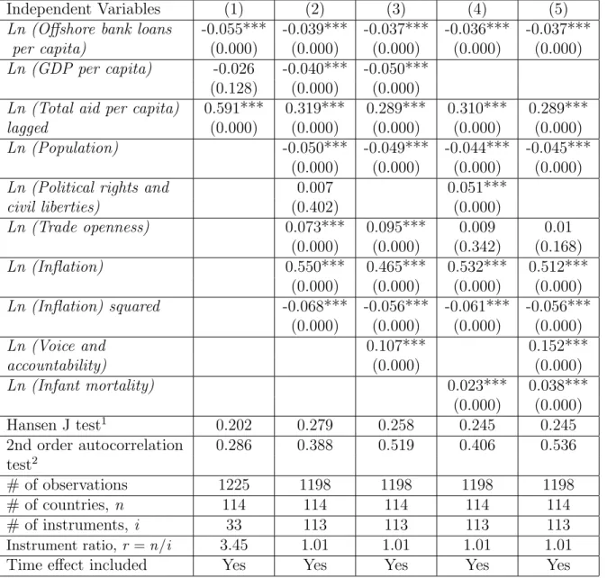
Tables 2-4 present results for aid equation. In Table 2, Column (1) reports the results of our baseline model, where we include log loans per capita, log GDP per capita and the lagged value of log total aid per capita. Consistent with the prediction of our theoretical model, the coefficient of log loans per capita is negative and statistically different from zero at the 1% level. As expected, the coefficient of log GDP per capita is also negative, but it is not statistically significant. The effect of lagged log aid per capita is positive and significant, implying persistence in aid allocation over time.
Column (2) reports results for the fully specified model by including other control vari-ables. The coefficient of log loans per capita remains negative and significant at the 1% level, suggesting that a higher inflow of foreign loans is associated with a lower aid allocation. That is, developing countries having better access to foreign credits receive less foreign aid.
The negative coefficient of log GDP per capita also becomes statistically significant at the 1% level, which is consistent with the previous finding that poor countries receive more aid. A negative and significant coefficient of log population confirms the bias in aid allocation to the small countries. Both trade openness and inflation positively impact aid, while the negative coefficient of the squared term of log inflation underscores its diminishing effect. As expected, better conditions of political rights and civil liberties positively influence aid, but their effects are not statistically significant.
21Data on some observations for some variables also exhibit negative values. Following others in the
literature, we linearly transform all variables by adding a constant in their values so that their lowest value equals zero.
As a robustness check, in column (3), we drop the political rights and civil liberties vari-able and instead include an alternative measure of democracy “log voice and accountability”, which has positive and significant impact on aid at the 1% level. Likewise, in columns (4) and (5), we replace log GDP per capita with log infant mortality rate. The positive and significant impact of infant mortality rate confirms that, all else equal, poverty remains a key criterion for aid allocation. The significance of political rights and civil liberties in col-umn (4) and voice and accountability in colcol-umn (5) further confirms that more democratic regimes are rewarded with aid. In each regression in Table 2, both the Hansen J and 2nd order autocorrelation tests confirm the validity of the instruments and the absence of serial correlation, respectively.
The inclusion of the new control variables in our fully specified models in columns (2-5) leaves the coefficient of the loans per capita negative, robust at around 0.037 and statistically significant at the 1% level. This suggests that a one percent increase in loans per capita is associated with a 0.037 percent decline in aid per capita. In monetary terms, this amounts to a reduction of total aid per capita of 2.091 USD for the average, and 1.270 USD for the median country in our sample. Note that in both columns (3) and (4), the estimated coefficient of lagged log aid per capita is 0.289, while the estimated coefficient of log loans per capita is 0.037. Thus, the long run effect on aid per capita is 0.052 (= 0.037/(1 - 0.289)), which implies that the aid reduction effect of loans increases over time.
Let us consider an example to get a better sense of this aid reduction effect of loans. Take two countries in our study Mexico, who received the lowest (1.12 USD), and Cape Verde, who received the highest (328.43 USD) amount of average aid per capita over the sample period. Then a one percent increase in loans per capita will induce a reduction of aid per capita of 0.042 USD in the short run and 0.056 in the long run for Mexico; and this amounts stands at 12.152 USD in the short run and 16.422 in the long run for Cape Verde. In total dollar value, this reduces aid by 4.217 million USD in the short run and
5.622 million USD in the long run for Mexico, while for Cape Verde this reduction in aid amounts to 5.564 million USD in the short run and 7.519 million USD in the long run. To offer yet another perspective, this reduces total aid by 76.830 million USD in the short run and 103.824 million USD in the long run for China, which is the most populous country in our sample. For Dominica, which is the least populous country in our sample, this reduction stands at 0.806 million USD in the short run and 1.089 million USD in the long run.
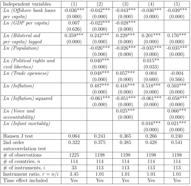
Next we examine whether the influence of loans on aid changes when we replace our dependent variable log total aid per capita with log bilateral aid per capita in Equation (16). The results in Table 3 show that log loans per capita has both quantitatively and qualitatively approximately the same effect on log bilateral aid per capita as for log total aid per capita in Table 2. This is true both for our baseline model as well as for our fully specified models. In fact, the magnitude of the coefficient of log loans per capita shows a marginal decrease from 0.037 to 0.043 in our fully specified model in column (3). In monetary terms, this amounts to a reduction of bilateral aid per capita of 1.525 USD for the average, and 1.476 USD for the median country in our sample. This long run effect is 0.056 (= 0.043/(1 - 0.229)), which, further strengthens our findings that the aid reduction effect of loans increases over time. The sign, significance, and interpretation of all other control variables remain the same as above.22
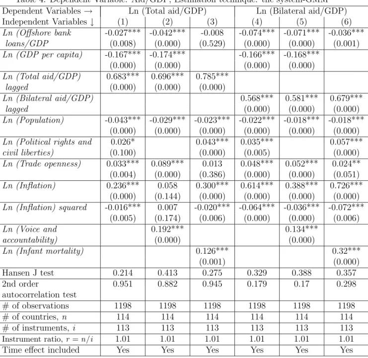
Finally, we run regressions by redefining our dependent variables as log total aid/GDP, log bilateral aid/GDP, and our key independent variable as log loans/GDP. We use log transformations of these variables for the same reasons as mentioned above. Table 4 reports the estimation results of the fully specified models for both log total aid/GDP and for log bilateral aid/GDP. In 5 out of 6 regressions, the coefficients of log loans/GDP remain negative and significant at the 1% level. These results further strengthen our findings in Tables 2 and 3 and, hence, our theoretical prediction that better access to foreign credits
22The variable of political rights and civil liberties which was statistically insignificant in column (2) of
reduces flow of aid to the developing countries. In fact, these findings suggest that the aid reduction influence of loans is substantially larger. For example, the size of the coefficient of log loans/GDP is 0.042 in log total aid/GDP regression in column (2), and its size is 0.071 for log bilateral aid/GDP regression in column (5). This suggests that the long run aid reduction effect of loans is 0.138 (= 0.042/(1 - 0.696)) for total aid/GDP, while it is 0.169 (= 0.071/(1 - 0.581)) for bilateral aid/GDP. The findings of all other control variables are as expected.
3.2
Borrowing, foreign aid and growth
3.2.1 Description of data and the empirical model
In this section, we test the first proposition of our theoretical model that at low (high) levels of borrowing and foreign aid, an increase in foreign aid has a bigger (smaller) effect on recipient welfare than an equivalent relaxation in the borrowing constraint. Following the empirical literature on aid-growth, we use growth rate of real GDP per capita to measure welfare (e.g., Arndt et al., 2010; Burnside and Dollar, 2000; Hansen and Tarp, 2001). The main variables of interests for testing this proposition are foreign aid and foreign loans.
Our empirical methodology still rests on the application of dynamic panel model based on the system-GMM estimator as employed for aid regressions in Table 2-4. This method has also been favored by several other recent contributions in aid-growth literature (e.g., Arndt
et al., 2010; Asiedu and Nandwa, 2007; Hansen and Tarp, 2001). Our empirical strategy
of using log-log model and, thus, necessary transformations of variables exhibiting negative values remains the same as discussed above in section 3.1.
Our empirical growth model takes the following form:
ln(growth)it = β0+β1ln(aid)it+β2(ln(aid))2it+β3ln(loans)it+β4(ln(loans))2it
where subscripts i refers to countries, t to time, κi to the country-specific effects, τt to the
time-effect,Z to the vector of control variables, andµit to the disturbance term. Once again
we use two alternative measures for aid and loans: in per capita terms and as percentage of GDP. Our main variables of interests in equation (17) are: log aid, log loans, (log aid)2 and (log loans)2. Based on the first proposition of our theoretical model, we hypothesize that
β1 > 0, β2 < 0, β3 < 0, and β4 > 0. That is, if these four coefficients turn out to be as
hypothesized, then the marginal effect of aid is higher (lower) than that of loans when the magnitude of these two variables is small (large).
With regards to the selection of control variable, we take guidelines from the recent aid-growth literature (e.g., Arndt et al., 2010; Asiedu and Nandwa, 2007; Burnside and Dollar, 2000; Hansen and Tarp, 2001). Specifically, we include: log fixed capital formation as proxied by investment/GDP, log initial real GDP per capita, log inflation and its squared term, log government consumption/GDP, log secondary school enrollments, log rule of law and the lagged value of log growth rate of real GDP per capita. Rule of law reflects the strength and impartiality of the legal system, as well as the enforcement of property rights. For robustness analysis, we also replace log initial real GDP per capita with log infant mortality rates.
Many influential past studies conclude that countries’ institutions are important for their economic growth and poverty alleviation (e.g., Acemoglu et al., 2001; Rodrik et al., 2004). Thus, we also employ alternative measures of institutional quality to examine whether the results of our main variables of interest remain robust with their inclusion. Data for the rule of law and other institutional measures such as regulatory quality and government effectiveness are taken from Kaufmann et al. (2009). A higher score of these institutional indices indicates better quality.23 Data for all the other control variables come from WDI
(2010). The descriptive statistics of all these variables are presented in Table 1.
23While regulatory quality captures the ability of the government to formulate and implement sound
policies and regulations promoting private sector development, government effectiveness mainly measures the quality of public services and the degree of its independence from political pressures.
3.2.2 Estimation results
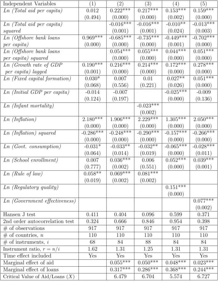
Tables 5-8 report the results. In table 5, column (1) presents the estimation results of the model that includes log total aid per capita and log loans per capita but not their squared terms; it, however, includes all other standard control variables. We find that while the coefficient of log loans per capita is positive and significant at the 1% level, the effect of log aid per capita is not statistically significant. This finding of aid is consistent with Boone (1996), who concludes that aid has no significant impact on macroeconomic variables. Boone’s empirical results, however, have been questioned by subsequent studies, which, unlike Boone, model aid-growth relation in the non-linear form (e.g., Burnside and Dollar, 2000; Durbarryet al., 1998; Hadjimichael et al., 1995; Hansen and Tarp, 2001).
Column (2) presents estimation results of our fully specified model which also includes squared terms of both log total aid per capita and log loans per capita. The positively signif-icant coefficient of log total aid per capita and negatively signifsignif-icant coefficient of its squared term confirm diminishing marginal returns to aid. This suggests that while some countries may utilize aid effectively, others lack the absorptive capacity or institutional quality with which to complement aid. This also indicates that after reaching a threshold level, the nega-tive rent seeking effect of aid dominates its posinega-tive infrastructure building effect, as pointed out in Harms and Lutz (2006).24 On the other hand, the negative significant coefficient of log
loans per capita and positive significant coefficient of its squared term suggests an increasing marginal return to loans. The signs of the coefficients of these main variables of our interests agree with our prior.
We evaluate the marginal effect of aid on growth (β1+ 2β2 Aid) at the mean value of aid
per capita, 5.23.25 We also evaluate this effect at its median value, 5.17, to deal with the
24See Hansen and Tarp (2001) for a detailed discussion on the theoretical arguments about non-linear effect
of aid on economic growth, which relate to absorptive capacity constraints, Dutch disease and institutional destruction problems in developing countries.
25For every regressions, the marginal effect of aid at its mean value (along with the significance of the
problem of skewed distribution of aid across countries and time. These calculations show that a one percent increase in the aid per capita induces an increase of roughly 0.05 percent in growth when this effect is evaluated at its mean value, and it spurs about 0.06 percent of growth when evaluated at its median level. Interestingly, this marginal impact of aid does not turn negative even when it is evaluated at a very high value of aid in our sample. For example, this effect is 0.04% when evaluated at 90th percentile of aid. This suggests that although aid is most effective at low level and its marginal effect decreases quite fast, it never has a growth demoting effect in our sample countries and time periods. This finding appears to appeal to the morals of giving aid as underscored by Stern (1974), who argues for the transfer from the better-off to the worse-off countries if the benefit to the latter justifies the cost to the former.
Next we evaluate the marginal effect of loans on growth (β3 + 2β4 Loans). Notice that
both mean, 9.28, and median, 9.27, values of loans per capita are approximately the same; therefore, we report its marginal effect evaluated at its mean value.26 This marginal effect of loans per capita on growth is 0.32, which is 84.38 percent higher than the marginal effect of aid per capita at its mean. This implies that starting at the mean level, an increase in aid will result in a decline in its positive effect on growth, while an increase in loans will augment its positive effect on growth. This, however, also implies that starting at a low level, aid has a larger positive effect on growth than loans. In fact, the negative effect of loans does not turn positive until it attains a fairly large value. These findings agree with the first proposition of our theoretical model.
The marginal effects of aid and loans computed above have been at their respective mean and median values. However, it is of interest to compute the critical level of financial transfer (either aid or loans) below (above) which the marginal effect of aid (loans) is larger. To do so we need to compute the value of X such thatβ1+ 2β2∗X =β3+ 2β4∗X. For column 2
26Like aid, the marginal effect of loans (along with the significance of the marginal effect) is also reported
of table 5, the value ofX is computed as 6.479 which is higher than the mean value of total aid per capita and lower than the mean value of loans per capita.27
Many past studies state that a change in control variables can change the results in growth regression (see, for example, Dollar and Levin, 2004). Thus, we check whether the results of our variables of interest are robust to the introduction of alternative controls that explain growth. In column (3), we replace log initial GDP per capita with log infant mortality rates. Next, we replace log rule of law with log regulatory quality and log government effectiveness, one at a time (see columns 4 and 5). These results show that sign, significance and even the magnitude of the coefficients of the variables of our interest remain the same with the inclusion of other control variables.
We now briefly discuss the results of control variables. Our results strongly support the findings of Hansen and Tarp (2001) that the lagged growth rate has a robust and positive effect on its current rate as its estimated coefficients are significant at the 1% level in all the regressions. Although domestic investment as proxied by fixed capita formation positively affect growth, but its statistical significance is not robust across all the specifications. As expected, initial GDP per capita, infant mortality rates and government consumption nega-tively influence growth, while school enrollment posinega-tively affects growth. Our findings also support the assertion of Rodrik et al. (2004) that institutions are important for growth as the coefficients of rule of law, regulatory quality and government effectiveness are positive and significant at the 1% level. Lastly, the sign and significance of the coefficients of inflation and its squared term reflect its diminishing effect.
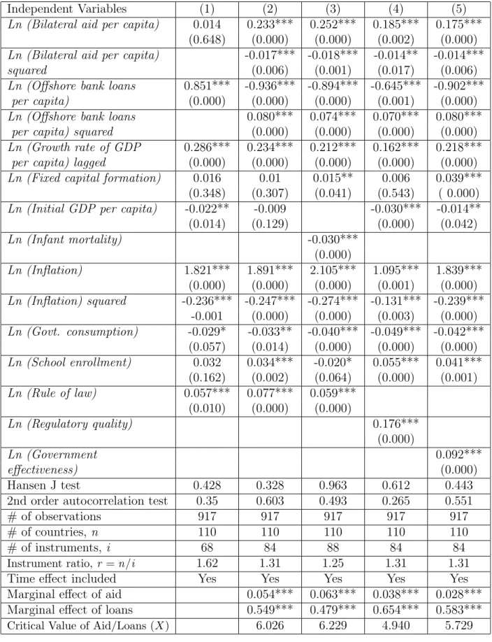
Next we replace log total aid per capita with log bilateral aid per capita as the former also includes part of multilateral assistance. The results in Table 6 show that the nonlinear effect of bilateral aid per capita is both quantitatively and qualitatively the same as that of total
27We also compute these values for all our regressions in which the squared values of Aid and Loans
aid per capita, which further confirms decreasing marginal returns to aid. Like aid per capita, this positive effect on growth decreases, but it never becomes negative even at the maximum value of bilateral aid per capita in our sample. For example, in the regression results in column (2), the partial effect of log bilateral aid per capita evaluated at its maximum value in our sample (6.37) stands at 0.02.
The negative significant coefficient of log loans per capita and positive significant coef-ficient of its squared term in all the regressions further confirm increasing returns to loans. Table 6 also shows that, for all the regressions, the partial effect of loans per capita evaluated at its mean value is between 40 and 58 percent larger than the partial effects calculated in Table 5. These results further strengthen our key assertion that the effectiveness of aid in fostering economic growth is higher at lower levels, while the effectiveness of loans is higher at higher levels. Similar examples given for the results in Table 5 above to elucidate the first proposition of our theoretical model can be replicated in the case for results in Table 6. The estimated results of all other control variables are as expected and agree with our prior.
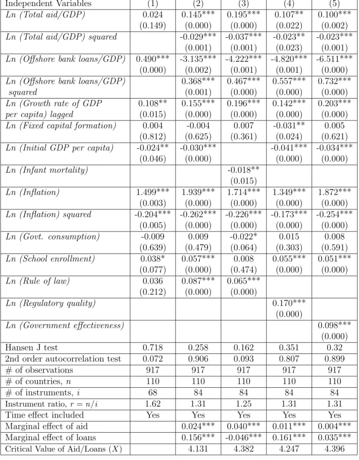
Finally, we take our main variables of interest as percentage of GDP: log total aid/GDP, log bilateral aid/GDP, log offshore bank loans/GDP and their respective squared terms. These results are presented in Table 7 and 8. In all the regressions, the sign and significance of the coefficients of aid and loans variables strongly confirm their non-monotonic relationship with growth, as found in the case of these variables in per capita form.
4
Conclusion
Should foreign aid be replaced by an easier access to international credit? Many in the past have argued an affirmative answer to this question. The argument lies partly on the belief that foreign aid is ineffective and partly on the argument that loans give more incentives to the recipients to utilize them wisely. Whether aid is ineffective is a moot point in the first
place. Second, whether loans have been effective in the past is also a moot point, as we have witnessed several financial crises involving developing countries.
In this paper we revisit these issues in a unified way. First of all we develop a theoretical model to examine the effect of both foreign aid and loans on the welfare of the recipient country. We also examine the interaction between foreign aid and loans. Our theoretical model has two periods and two countries: a recipient and a donor. The recipient country is subject to a binding borrowing constraint and the donor is altruistic toward the recipient. Foreign aid is given for the purpose of providing a public input; however, the recipient is able to optimally divert a proportion of it as lump-sum payments to the consumers. We find that both foreign aid and a relaxation of the borrowing constraint increase the welfare of the recipient. However, the marginal effect of a loan is larger than that of foreign aid if and only if the initial level of that transfer is sufficiently large. We also consider the case where the amount of foreign aid is optimally chosen by the donor, and find that a relaxation of the borrowing constraint reduces the equilibrium level of foreign aid.
Having established the above-mentioned propositions, we then test them using data. We use annual data for the period 1997-2008 for 114 aid-recipient countries. The sources are the OECD, the World Bank, Freedom House, Kaufmann et al. (2009), and the Bank of International Settlement. We employ a dynamic panel generalized method of moments (GMM) analysis to our data set, mainly to address the endogeneity problem in multiple variables. We use various controls apart from the main variables of interest and use different definitions of the main variables: aid per capita, loans per capita, aid as a proportion of GDP, and loans as a proportion of GDP. All of our regressions point to a robust non-linear relationship between growth and aid and between growth and loans. In particular, we find strong support for our theoretical prediction that there is a critical value of money transfer, and if the initial levels of loans or aid are lower than this critical level, then the marginal effect of foreign aid is larger than that of loans. We also find strong support of our other theoretical prediction that more loans do reduce the level of foreign aid.
References
[1] Acemoglu, D., Johnson, S. and Robinson, J. A. (2001). “The colonial origins of com-parative development: an empirical investigation,” American Economic Review, 91, 1369-1401.
[2] Alesina, A. and Dollar, D. (2000). “Who gives foreign aid to whom and why?” Journal
of Economic Growth, 5, 33-63.
[3] Addison, T., Mavrotas, G. and McGillivray, M. (2005) “Development assistance and development finance: evidence and global policy agendas,” Journal of International
Development, 17, 819-836.
[4] Arellano, M. and Bond, S. R. (1991). “Some tests of specification for panel data: monte carlo evidence and an application to employment equations,”Review of Economic Stud-ies, 58, 277–97.
[5] Arellano, M. and Bover, O. (1995). “Another look at the instrumental variable estima-tion of error components Models,” Journal of Econometrics, 68, 29-52.
[6] Arndt, C., Jones, S. and Tarp, F. (2010). “Aid, growth, and development: have we come full circle?” Journal of Globalization and Development, 1, Article 5.
[7] Asiedu, E. and Nandwa, B. (2007). “On the impact of foreign aid in education on growth: How relevant is the heterogeneity of aid flows and the heterogeneity of aid recipients?” Review of World Economics, 143, 631-649.
[8] Asiedu, E. and Lien, D. (2011). “Democracy, foreign direct investment, and natural resources.” Journal of International Economics, 84, 99-111.
[9] Baliamoune-Lutz, M. and Mavrotas, G. (2009). ”Aid effectiveness: looking at the aid– social capital–growth nexus,” Review of Development Economics, 13, 510-525.
[10] Bandyopadhyay, S., Sandler, T. and Younas, J. (2011). “Foreign direct investment, aid, and terrorism: an analysis of developing countries,” Unpublished manuscript, Center for Global Collective Action, University of Texas at Dallas.
[11] Bauer, P.T. (1971). Dissent on Development, London: Widenfeld and Nicolson.
[12] Beck, T., Demirg¨u¸c-Kunt, A. and Levine, R. (2000). “A new database on financial development and structure,” World Bank Economic Review, 14, 597-605.
[13] Beck, T. and Demirg¨u¸c-Kunt, A. (2009). “Financial institutions and markets across countries and over time: data and analysis”, World Bank Policy Research Working Paper No. 4943.
[14] Bigsten, A., Collier, P., Dercon, S., Fafchamps, M., Gauthier, B., Gunning, J., Oduro, A., Oostendorp, R., Patillo, C., S–derbom, M., Teal, F. and Zeufack, A. (2003). “Credit constraints in manufacturing enterprises in Africa,” Journal of African Economies 12, 104-125.
[15] Blundell, R. and Bond, S. (1998). “Initial conditions and moment restrictions in dynamic panel models,”Journal of Econometrics, 87, 115-143.
[16] Boone, P. (1996). “Politics and the effectiveness of foreign aid,” European Economic
Review, 40, 289-329.
[17] Burnside. C. and Dollar. D. (2000). “Aid, policies, and growth,” American Economic
Review, 90, 847-868.
[18] Chenery, H.B. and Strout, A.M. (1966). “Foreign assistance and economic develop-ment,” American Economic Review, 56, 679-733.
[19] Chor, D. and Manova, K. (2011). “Off the cliff and back? credit conditions and inter-national trade during the global financial crisis, Journal of International Economics, forthcoming.
[20] Collier, P. and Dollar. D. (2002). “Aid allocation and poverty reduction,” European
Economic Review, 45, 1-26.
[21] Dollar, D. and Levin, V. (2004). “The increasing selectivity of foreign aid, 1984-2002,” World Bank Policy Research Paper 3299.
[22] Dalgaard, C.J., Hansen, H. and Tarp, F. (2004). ”On the empirics of aid and growth,”
Economic Journal, 114, 191-216.
[23] Dixit, A., and Norman, V. (1980). Theory of International Trade, Cambridge: Cam-bridge University Press.
[24] Dreher, A., Sturm, J. and Vreeland, J. R. (2009). “Development aid and international politics: does membership on the UN Security Council influence World Bank decision?”
Journal of Development Economics, 88, 1-18.
[25] Dudley, L. and Montmarquette, C. (1976). “A model of supply of bilateral aid foreign aid,” American Economic Review, 66, 132-142.
[26] Durbarry, R., Gemmell, N. and Greenaway, D. (1998). “New evidence on the impact of foreign aid on economic growth,” CREDIT Research Paper 98r8, University of Notting-ham.
[27] Easterly, W. (2003). “Can foreign aid buy growth?” Journal of Economic Perspectives
17, 23-48.
[29] Feyzioglu, T., Swaroop, V. and Min, Z. (1998). “A panel data analysis of the fungibility of foreign aid,” The World Bank Economic Review, 12, 29–58.
[30] Galindo, A. and Schiantarelli, F. (editors) (2003) Credit constraints and investment in
Latin America, Inter-American Development Bank, Washington, DC.
[31] Hadjimichael, M.T., Ghura, D., M¨uhleisen, M., Nord, R. and Ucer, E.M. (1995). “Sub-Saharan Africa: growth, savings, and investment, 1986-93,” Occasional Paper 118, In-ternational Monetary Fund.
[32] Hansen, H. and Tarp, F. (2000). “Aid effectiveness disputed,”Journal of International
Development, 12, 375-398.
[33] Hansen H. and Tarp, F. (2001). “Aid and growth regressions,”Journal of Development
Economics, 64, 547–570.
[34] Harms, P. and Lutz, M. (2006). “Aid, governance and private foreign investment: some puzzling findings for the 1990s,” Economic Journal, 116, 773-790.
[35] Harrison, A. and McMillan, M. (2003) Does direct foreign investment affect domestic credit constraints?” Journal of International Economics, 61, 73-100.
[36] H´ericourt, J. and Poncet, S. (2007). “FDI and credit constraints: firm level evidence in China,” Universit´e Paris I Panth´eon-Sorbonne - TEAM, February.
[37] Hermann, S. and Mihaljek, D. (2011). “The determinants of cross-border bank flows to emerging markets: new evidence on the spread of financial crises,” Bank of Finland Working Paper No. 3-2011.
[38] Kaufmann, D., Kraay, A. and Mastruzzi, M. (2009). “Governance matters VII: gover-nance indicators for 1996-2008,” World Bank Policy Research, June 2009.
[39] Kuziemko, I. and Werker, E. (2006). “How much is a seat on the Security Council worth? Foreign aid and bribery at the United Nations,” Journal of Political Economy, 114, 905-930.
[40] Lahiri, S. (ed.) (2006).Theory and Practice of Foreign aid (Frontiers of Economics and
Globalization, Volume 1), Emerald Group Publishing Limited.
[41] Lahiri, S., and Raimondos-Møller, P. (1997). “Competition for aid and trade policy,”
Journal of International Economics, 43, 369-385.
[42] Mavrotas, G. (2006). “Scaling up of foreign aid and the emerging new agenda,” Chapter 13 in Lahiri, S. (ed.), Theory and Practice of Foreign aid (Frontiers of Economics and
Globalization, Volume 1), Emerald Group Publishing Limited, pp. 211-233.
[43] Maizels, A. and Nissanke, M. (1984). “Motivations for aid to developing countries,”
World Development, 12, 879-900.
[44] McGillivray, M., Feeny, S., Hermes, N. and R. Lensik. (2006). “Controversies over the impact of development aid: it works; it doesn’t work; it can, but that depends. . . ,”
Journal of International Development, 18, 1031-1050.
[45] Papaioannou, E. (2009). “What drives international financial flows? politics, institu-tions and other determinants,”Journal of Development Economics, 88, 269-281. [46] Rajan, R. and Zingales, L. (1998) “Financial dependence and growth,”American
Eco-nomic Review, 88, 559-586.
[47] Rajan, R. and Subramanian, A. (2005) “Aid and growth, what does the cross-country evidence really show?” IMF Working Paper No. 05/127.
[48] Rodrik, D., Subramanian, A. and Trebbi, F. (2004). “Institutions rule: the primacy of institutions over geography and integration in economic development,” Journal of
Economic Growth, 9, 131-165.
[49] Roodman, D. (2007). “A short note on the theme of too many instruments,” Center for Global Development, Working Paper 125.
[50] Stern, N.H. (1974). “Professor Bauer on development: a review article,” Journal of
Development Economics, 1, 191-211.
[51] Swaroop, V., Jha, S., Rajkumar, A.S. and Sunil, A. (2000). “Fiscal effects of foreign aid in a federal system of governance: the case of India”.Journal of Public Economics, 22, 307–330.
[52] Trumbull, W.N. and Wall, H.J. (1994). “Estimating aid allocation criteria with panel data,” Economic Journal, 104, 876-882.
[53] Wilson, J.D. (1991). “Optimal public good provision with limited lump-sum taxation,”
American Economic Review, 81, 153-66.
[54] World Bank (2010), World Development Indicators, 2010. World Bank, Washington, DC.
[55] Younas, J. and Bandyopadhyay, S. (2009). “Do donors care about declining trade rev-enue from liberalization? An analysis of bilateral aid allocation,” Federal Reserve Bank
of St. Louis Review, 91, 141-153.
[56] Younas, J. (2008). “Motivation for bilateral aid allocation: altruism or trade benefits,”
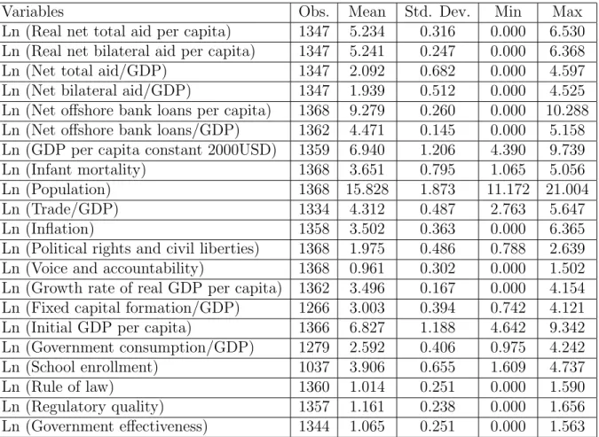
Table 1: Summary statistics for variables used in aid (Equation 16) as well as in growth regressions (Equation 17).
Variables Obs. Mean Std. Dev. Min Max
Ln (Real net total aid per capita) 1347 5.234 0.316 0.000 6.530 Ln (Real net bilateral aid per capita) 1347 5.241 0.247 0.000 6.368 Ln (Net total aid/GDP) 1347 2.092 0.682 0.000 4.597 Ln (Net bilateral aid/GDP) 1347 1.939 0.512 0.000 4.525 Ln (Net offshore bank loans per capita) 1368 9.279 0.260 0.000 10.288 Ln (Net offshore bank loans/GDP) 1362 4.471 0.145 0.000 5.158 Ln (GDP per capita constant 2000USD) 1359 6.940 1.206 4.390 9.739 Ln (Infant mortality) 1368 3.651 0.795 1.065 5.056 Ln (Population) 1368 15.828 1.873 11.172 21.004 Ln (Trade/GDP) 1334 4.312 0.487 2.763 5.647 Ln (Inflation) 1358 3.502 0.363 0.000 6.365 Ln (Political rights and civil liberties) 1368 1.975 0.486 0.788 2.639 Ln (Voice and accountability) 1368 0.961 0.302 0.000 1.502 Ln (Growth rate of real GDP per capita) 1362 3.496 0.167 0.000 4.154 Ln (Fixed capital formation/GDP) 1266 3.003 0.394 0.742 4.121 Ln (Initial GDP per capita) 1366 6.827 1.188 4.642 9.342 Ln (Government consumption/GDP) 1279 2.592 0.406 0.975 4.242 Ln (School enrollment) 1037 3.906 0.655 1.609 4.737 Ln (Rule of law) 1360 1.014 0.251 0.000 1.590 Ln (Regulatory quality) 1357 1.161 0.238 0.000 1.656 Ln (Government effectiveness) 1344 1.065 0.251 0.000 1.563 Note: Data for all variables range from 1997-2008. All of the ratios are defined as per-centage of GDP. Total aid is the sum of bilateral and multilateral aid. Loans data from Bank for International Settlement (BIS) is adjusted for exchange rate movements (done by BIS).
Table 2: Dependent variable: Ln (Total aid per capita); Estimation technique: the system-GMM
Independent Variables (1) (2) (3) (4) (5)
Ln (Offshore bank loans -0.055*** -0.039*** -0.037*** -0.036*** -0.037***
per capita) (0.000) (0.000) (0.000) (0.000) (0.000)
Ln (GDP per capita) -0.026 -0.040*** -0.050***
(0.128) (0.000) (0.000)
Ln (Total aid per capita) 0.591*** 0.319*** 0.289*** 0.310*** 0.289***
lagged (0.000) (0.000) (0.000) (0.000) (0.000)
Ln (Population) -0.050*** -0.049*** -0.044*** -0.045***
(0.000) (0.000) (0.000) (0.000)
Ln (Political rights and 0.007 0.051***
civil liberties) (0.402) (0.000) Ln (Trade openness) 0.073*** 0.095*** 0.009 0.01 (0.000) (0.000) (0.342) (0.168) Ln (Inflation) 0.550*** 0.465*** 0.532*** 0.512*** (0.000) (0.000) (0.000) (0.000) Ln (Inflation) squared -0.068*** -0.056*** -0.061*** -0.056*** (0.000) (0.000) (0.000) (0.000) Ln (Voice and 0.107*** 0.152*** accountability) (0.000) (0.000) Ln (Infant mortality) 0.023*** 0.038*** (0.000) (0.000) Hansen J test1 0.202 0.279 0.258 0.245 0.245 2nd order autocorrelation 0.286 0.388 0.519 0.406 0.536 test2 # of observations 1225 1198 1198 1198 1198 # of countries, n 114 114 114 114 114 # of instruments,i 33 113 113 113 113 Instrument ratio,r =n/i 3.45 1.01 1.01 1.01 1.01
Time effect included Yes Yes Yes Yes Yes
Notes for this and all subsequent tables: We employ two-step estimation for the
system-GMM, which is considered asymptotically efficient and robust to all kinds of heteroskedasticity.
Superscripts ∗∗∗, ∗∗, and ∗ indicate significance at the 1, 5, and 10% levels, respectively. P values
are in parentheses.
1 The null hypothesis is that the instruments are not correlated with the residuals. (P values)