VYSOKÉ U
Č
ENÍ TECHNICKÉ V BRN
Ě
BRNO UNIVERSITY OF TECHNOLOGYFAKULTA INFORMA
Č
NÍCH TECHNOLOGIÍ
ÚSTAV PO
Č
ÍTA
Č
OVÉ GRAFIKY A MULTIMÉDIÍ
FACULTY OF INFORMATION TECHNOLOGY
DEPARTMENT OF COMPUTER GRAPHIC AND MULTIMEDIA
ADABOOST IN COMPUTER VISION
DIPLOMOVÁ PRÁCE
MASTER‘S THESISAUTOR PRÁCE
B
C.
M
ICHALH
RADIŠAUTHOR
VYSOKÉ U
Č
ENÍ TECHNICKÉ V BRN
Ě
BRNO UNIVERSITY OF TECHNOLOGYFAKULTA INFORMA
Č
NÍCH TECHNOLOGIÍ
ÚSTAV PO
Č
ÍTA
Č
OVÉ GRAFIKY A MULTIMÉDIÍ
FACULTY OF INFORMATION TECHNOLOGY
DEPARTMENT OF COMPUTER GRAPHIC AND MULTIMEDIA
ADABOOST V PO
Č
ÍTA
Č
OVÉM VID
Ě
NÍ
ADABOOST IN COMPUTER VISIONDIPLOMOVÁ PRÁCE
MASTER‘S THESISAUTOR PRÁCE
Bc. Michal Hradiš
AUTHOR
VEDOUCÍ PRÁCE
Ing. Igor Potú
č
ek, Ph.D.
SUPERVISOR
Abstrakt
V této diplomové práci jsou představeny nové obrazové příznaky „local rank differences“ (LRD).
Tyto příznaky jsou invariantní vůči změnám osvětlení a jsou vhodné k implementaci detektorů
objektů v programovatelném hardwaru, jako je například FPGA. Chování klasifikátorů s LRD
vytvořených pomocí algoritmu AdaBoost bylo otestováno na datové sadě pro detekci obličejů. LRD
v těchto testech dosáhly výsledků srovnatelných s výsledky klasifikátorů s Haarovými příznaky, které
jsou používány v nejlepších současných detektorech objektů pracujících v reálném čase. Tyto
výsledky ve spojení s faktem, že LRD je možné v FPGA vyhodnocovat několikanásobně rychleji než
Haarovy příznaky, naznačují, že by LRD příznaky mohly být řešením pro budoucí detekci objektů
v hardwaru. V této práci také prezentujeme nástroj pro experimenty s algoritmy strojového učení
typu boosting, který je speciálně uzpůsoben oblasti počítačového vidění, je velmi flexibilní, a přitom
poskytuje vysokou efektivitu učení a možnost budoucí paralelizace výpočtů. Tento nástroj je
dostupný jako open source software a my doufáme, že ostatním ulehčí vývoj nových algoritmů a
příznaků.
Klí
č
ová slova
In this thesis, we present the local rank differences (LRD). These novel image features are invariant to lighting changes and are suitable for object detection in programmable hardware, such as FPGA. The performance of AdaBoost classifiers with the LRD was tested on a face detection dataset with results which are similar to the Haar-like features which are the state of the art in real-time object detection. These results together with the fact that the LRD are evaluated much faster in FPGA then the Haar-like features are very encouraging and suggest that the LRD may be a solution for future hardware object detectors. We also present a framework for experiments with boosting methods in computer vision. This framework is very flexible and, at the same time, offers high learning performance and a possibility for future parallelization. The framework is available as open source software and we hope that it will simplify work for other researchers.
Keywords
Boosting, AdaBoost, Local Rank Differences, LRD, Computer Vision, Face Detection, Haar-like Features, WaldBoost,
Citace
AdaBoost in Computer Vision
Prohlášení
Prohlašuji, že jsem tuto diplomovou práci vypracoval samostatně pod vedením Ing. Igora Potúčka,
Ph.D. a uvedl jsem všechny literární prameny a publikace, ze kterých jsem čerpal.
……… Michal Hradiš
© Michal Hradiš, 2007.
Tato práce vznikla jako školní dílo na Vysokém učení technickém v Brně, Fakultě informačních technologií. Práce je chráněna autorským zákonem a její užití bez udělení oprávnění autorem je nezákonné, s výjimkou zákonem definovaných případů.
Acknowledgements
First of all, I would like to express my thanks to Adam Herout for directing my interests towards computer graphic and later also towards computer vision and for helping me in many ways during my work on this thesis. I am very grateful to Igor Potúček, Víťa Beran, Jana Šilhavá, Michal Seman,
Michal Španěl and all the other people at UPGM for providing great inspiration and for their help
with increasing my knowledge of computer vision and machine learning. Especially, I would like to thank Pavel Zemcik for many interesting and guiding discussions and for the opportunity to
participate in the research at UPGM. I would like to thank Roman Juránek for his help with the boosting framework and his great support for the experiments we have performed.
A part the work was done at the Spring School on Image Processing in Szeged. I would like to thank my team mates Ilona Jedyk, Ágoston Róth and Sándor Szabó for their great work on the facial expression recognition demonstration application.
The work presented in this thesis has been financially supported by the Czech Science Agency grant “Algorithms of image recognition” GACR GA201/06/1821, IST EU grant CARETAKER – “Content Analysis and REtrieval Technologies to Apply Knowledge Extraction to massive Recording” EU-6FP-IST 027231, Czech Academy of Sciences Grant Agency grant “Rapid prototyping tools for development of HW-accelerated embedded image- and video-processing applications” GA AVCR, 1ET400750408, and Ministry of Education, Youth, and Sport grant “Research of information technologies form the security point of view”, CEZ MSMT, MSM 0021630528.
Contents
Contents ...1
1 Introduction...3
1.1 Introduction to Classification ...4
1.2 Classification Formalization...6
1.3 Limitations of Classification and Machine Learning ...6
2 Boosting ...8
2.1 AdaBoost...8
2.2 Real AdaBoost...9
2.3 AdaBoost Discussion ...11
2.4 Improving Learning Process ...13
2.5 Speed and Accuracy Tradeoff ...15
2.6 Learning Speedup...17
3 Data Transformations in Computer Vision ...18
3.1 Haar-like Features ...18
3.2 Gabor Features ...20
3.3 Local Binary Patterns ...21
3.4 Linear Transforms ...21
4 Weak Learning Algorithms...23
4.1 Histograms ...23
4.2 Decision Trees and Decision Stumps...24
5 New Image Features ...25
5.1 Min/Max Features ...26
5.2 Local Rank Differences...27
5.3 LRD in FPGA...28
6 Experimental Boosting Framework ...31
6.1 Requirements...31
6.2 Basic Principles ...33
6.3 Framework Structure...34
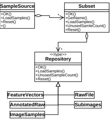
6.4 Data Source ...36
6.5 Features ...38
6.6 Weak Learners and Hypotheses ...38
6.7 The Boosting Algorithms and Cascade ...39
6.8 Potential for Parallelization ...39
6.10 Support Tools ...42
7 Results...43
7.1 Comparison of Different Types of Features...44
7.2 Threshold Estimation Precisions ...45
7.3 Restricting the Sizes of LRD...47
7.4 Prediction Value Quantization ...49
7.5 Convolution Quantization ...50
8 Conclusions and Future Work...52
1
Introduction
This thesis falls into the broad field of machine learning, which emerged from artificial intelligence research. Machine learning studies how to automatically extract information from data and possibly act according to that information. In the context of this work, learning is understood as inductive inference where rules and patterns are extracted from observed examples which incompletely represent some stochastic phenomenon. More specifically, the theme of this thesis is supervised machine learning, where each observed training example has an explicitly assigned label. The task of the learning method is then to create a prediction rule based on the information extracted form the training data and the corresponding labels. This prediction rule is then used to predict labels for unseen data samples. In general, the labels can be either discrete, in which case we speak about pattern classification – or real-valued in regression problems. Only classification is considered in this thesis.
Relatively recently, large margin classification methods emerged as practical results of statistical learning theory. Large margin classifiers search for such prediction rules which maximize distance of almost all examples from the decision boundary. The most theoretically and practically studied classes of large margin classifiers are support vector machines [1] (SVM) and boosting. In this thesis we focus on AdaBoost [2][3][4], which is one of the boosting methods, and its use in computer vision.
AdaBoost and its modifications have been successfully used in practical computer vision applications [5][6][7][8][9][10][11][12][13]. For example, the state of the art object detection classifiers are variations of cascade of boosted Haar-like features [7][8][9]. In object detection, image sub-windows on all positions, of different sizes and possibly rotations are scanned with a classifier. This results in very large number of classified image regions which places high demands on the computational effectiveness of the classifier. Haar-like features are very suitable for detection tasks as they can be computed very fast in constant time independent on their size using integral image [5][6]. In the considered approach, simple (weak) classifiers are each created based on a single Haar-like feature. AdaBoost then selects some of the weak classifiers and combines them into very accurate prediction rule. The prediction rule is a weighted majority vote of the weak classifiers and gets more accurate as more weak classifiers are added. This allows trade-off between classification accuracy and computational time. To optimize performance, some kind of cascade of consequently more complex classifiers is usually used. In such cascade, each stage rejects those image regions which are classified with enough confidence as background. Such cascade gradually lowers the false positive rate, which has to be very low in detection problems. In chapter 2, we give an overview of some boosting methods. Chapter 3 presents some of the data transformation techniques used in computer vision. Namely, the presented techniques are: principle component analysis (PCA), linear
discriminant analysis (LDA), Haar-like features, Gabor features and local binary patterns (LBP). Some of the commonly used weak learners are described in chapter 4.
Haar-like features offer high performance if the classifier is evaluated on general purpose CPU. On the other hand, they are not very suitable for FPGA1 and generally hardware implementation, which could be used in diverse embedded applications. The main issues preventing efficient implementation in FPGA are the need of normalization and the need of random memory access to each pixel of the integral image. Although, there exist some FPGA implementations of object detectors with Haar-like features [14][15][16], they provide relatively low performance. In chapter 5, we present new image features which could be effectively implemented in FPGA. Namely, the local rank differences [17] (LRD, see section 5.2) offer comparable discriminative power as Haar-like features, but the FPGA implementation [18] can evaluate one of these features in each clock cycle instead of six or eight cycles in the case of Haar-like features. Moreover, the LRD features do not require any explicit normalization as they implicitly normalize the results with local histogram equalization.
In the search for new features suitable for FPGA, it was necessary to create an experimental framework which could be used to evaluate performance of the newly suggested features. This framework has to be modular and has to offer high performance. Chapter 6 describes the framework. In chapter 7, we present many experimental results which were obtained using the framework. These results are mainly focused on the performance of the LRD. Finally, the achieved results are summarized and future work is suggested in chapter 0.
1.1
Introduction to Classification
Let’s now look at an example of supervised machine learning approach to a simple classification task. Imagine we need to create a machine which can distinguish between horses and zebras. Do not occupy your mind with the question why should we do such thing and let’s focus only on the question how to do it. Our classification machine will physically consist of a large black box with three doorways. One of the doorways will serve as entrance and the other two will serve as exits. Everything that leaves one exit will be considered a horse and everything that leaves the other exit will be further treated as a zebra. Inside the black box, there will be a computer to run our classification program (or prediction rule) and a hard-working but simple-minded2 person who will be able to perform simple routine measurements on the animal inside the box and enter the results of the measurements into the computer. We will call the person Sensor in the further text. To sum it up, the
1 Field-programmable gate array is a class of integrated circuits containing programmable logic components and
programmable interconnects.
operation of our classification machine will consist of following steps. After an animal enters the box, Sensor performs some measurements and enters the results into the computer running classification software. The classification software then decides the fate of the animal based on the data obtained from Sensor.
Now, as we have the basic structure of the classification machine, we need to decide what Sensor will measure and how the classification software will work. Let’s look at the measurements first. In machine learning, single measurement (or the measurable property of the phenomena being observed) is called a feature and a set of measurement results describing single object is called a feature vector. There are two basic requirements for the features used for classification. First, the set of features must be discriminative. Meaning the features should contain relevant information which can be used to distinguish between objects belonging to different classes. For example, a set of features consisting of the number of legs, the number of eyes and the weight of the animal does not contain much relevant information to distinguish between horses and zebras. On the other hand, a set of features describing all colors present on the animal skin and average length and width ratio of the colored patches should provide highly relevant information for our classification task. The features very much influence quality of the resulting classifier and their design offers great opportunity for human innovation.
The other usual requirement is to keep the number of features reasonably low. The obvious reason for doing so is computational complexity of the classifier. The computational complexity always grows – in some cases (e.g. artificial neural networks) even very fast – with the number of features for both classifier training and prediction rule evaluation. There is also the cost of the measurement itself, which can become very high in cases where specific sensors are needed or human involvement is necessary. An example of such area of applications is medical diagnostic, where each further examination can cost hundreds of Euros. In the case of our classification machine, there will be the problem with measurement cost too as we decided to use human to carry out the measurements. To reduce this cost, we will employ very simple-minded person. Because of this, we need to choose as simple and as well-defined features as possible, otherwise the measurement time may significantly reduce the throughput of the system. One of such simple features can be the number of light and dark transitions on the animal skin along a horizontal line. This feature itself should also be discriminative enough to distinguish between horses and zebras.
Next, we need to choose the classification method. This is another crucial point and the choice can influence the performance of the resulting application greatly. Classification methods can differ in the time needed for learning, computation complexity of the classifier, the complexity of the decision boundary, generalization properties (the performance on unseen data) and many other attributes. Some of the available classification methods are naive Bayes classifier, artificial neural networks, SVM, decision trees, AdaBoost, K-nearest neighbor and many others. In our case, we have
the advantage of having only one dimensional feature space. Moreover, we can assume that zebras have more light and dark transitions along the horizontal line then most of the horses have. So, it is not unreasonable to think that we can find a threshold for this feature which can separate horses from zebras with relatively low error.
The example of the machine classifying horses and zebras is very simple and we could set the threshold ourselves using only our intuition and very few examples. This way we would, in fact, become the learning algorithm ourselves. Obviously, this is not possible in more complex tasks where automatic learning algorithms must be used. Since, we want to discus machine learning, we will set the threshold automatically. To do so, we need the training examples first. We have to gather two separate herds of zebras and horses and let Sensor measure and note the number of intensity transitions on the skin of each animal. We also have to note which measurements belong to zebras and which belong to horses. Having this training data, we can easily automatically set the threshold value such that the classification error on the training data will be minimal. At this point, we have all the parts of the machine ready.
1.2
Classification Formalization
The task of machine learning algorithm in supervised classification problem is to find a rule (or hypothesis) which assigns an object to one of several classes based on external observations. Such prediction rule can be formalized as a function h:Χ→Υ where Χ is the input domain (the feature space) andΥis the set of possible labels. Let S=
(
x1,y1) (
,K, xm,ym)
be a set of training exampleswhere each instance xi belongs toΧand each yi belongs to Υ. When referring to single example, a
letter i is usually used. The training samples are usually supposed to be generated independent identically distributed (i.i.d) according to unknown probability distribution Ρ on Ζ=Χ×Υ. The task of the learning algorithm is then to estimate such function h which minimizes some objective error function on the training sample set S . Although, Υcan be an arbitrary finite set, we consider only binary classification in this thesis where Υ=
{
−1,+1}
.1.3
Limitations of Classification and Machine
Learning
There are many limitations on what can be achieved by machine learning methods in classification tasks. The first fundamental limitation is the fact that the true class-conditional probability density functions (PDF) of different classes can overlap. In other words it is possible that single data point in the feature space can be generated by objects from more than one class. The amount of the overlap
depends on what we can measure about the observed object. More or better sensors can in many cases solve this kind of difficulties, but this may not be feasible considering the costs.
Another limitation arises from the size of the feature space. Considering, we always have only a finite set of training examples, we are not able to estimate the true class-conditional PDFs exactly. This problem becomes more profound with higher number of dimensions. For example, in a small feature spaces (two or three dimensions), it would be possible to discretize the feature space and estimate the class-conditional PDFs for each of the discrete points with high accuracy using only moderate number of training examples. With higher number of dimensions, this approach becomes infeasible, because the number of examples needed for reliable PDF estimation becomes extremely high. To be more precise the size of the feature space increases exponentially with the number of dimensions. This exponential increase is sometimes referred to as the “curse of dimensionality” [19].
The final limitation is caused by our ability to acquire suitable training set. In machine learning, it is generally assumed that the samples from training set are generated i.i.d. according to the same probability distribution as the unseen samples. In practice, this assumption is often violated as it is not possible or affordable to obtain training set in exactly the same conditions as the resulting application will work in. The performance of the classifier then largely depends on the degree of similarity of the probability distributions from which both training and unseen samples are generated.
2
Boosting
The term boosting refers to a group of ensemble supervised learning algorithms. The basic idea of these algorithms is to iteratively combine relatively simple prediction rules (weak classifiers) into very accurate prediction rule (strong classifier). In most of the boosting algorithms, the weak classifiers are linearly combined. In the case of two-class classification, the strong classifier is the weighted majority of the votes. For introduction to boosting look at [3][4].
Boosting has its roots in the PAC (Probably Approximately Correct) machine learning model [20][21]. In this framework, the learner’s task is to find – with a high probability – a bounded approximation of a classification function using only training samples which are labeled by this particular function. The PAC model constrains the learning methods in terms of their effectiveness – the learning time must be polynomial-bounded as well as the number of needed training samples. The question, if a learning algorithm which performs just slightly better then random guessing in the PAC model can be boosted into arbitrarily accurate learning algorithm was first suggested by Kearns and Valiant [22][23]. The first polynomial-time boosting algorithms were introduced by Freund [24] and Schapire [25]. These early algorithm, however, suffered from many drawbacks. For example, they needed some prior knowledge of the accuracies of the weak classifiers and the performance bound of the final classifier depended only on the accuracy of the least accurate weak classifier.
The AdaBoost algorithm, which was first introduced by Freund and Schapire [2], solved most of the practical drawback of the earlier boosting algorithms. In the original algorithm the output of weak classifiers is restricted to binary value and thus the algorithm is referred to as discrete AdaBoost. Schapire and Singer [26] introduced real AdaBoost, which allows confidence rated predictions and is most commonly used in combination with domain-partitioning weak hypotheses (e.g. decision trees). The following text introduces the original AdaBoost algorithms and discusses their general properties and performance. In the further text, some modifications of the original algorithms are discussed mostly focusing on convergence speed, accuracy-speed trade-off and noise resistance.
2.1
AdaBoost
AdaBoost calls a given weak learning algorithm repeatedly in a series of rounds t=1,K,T . In
each iteration, the weak learning algorithm is supplied with different distribution D over the t
example set S . The task of the weak learner is to find a hypothesis ht :Χ→
{
−1,+1}
minimizing a classification error in respect to the current distribution D : t( )
[
t i i]
D i t =P~ t h x ≠ y ε (1)The weak hypothesis is then added to the strong classifier with a coefficient αt which is
selected according to the error εt of the hypothesis h on the current distribution t D : t − = t t t ε ε α ln 1 2 1
The final strong classifier is a linear combination of the selected weak hypothesis:
( )
=∑
= x h sign x H t T t t 1 ) ( αAfter a weak hypothesis is selected, new distributionDt+1 is generated in such way that the
weights of the samples which are correctly (respective wrongly) classified by ht decrees (respective
increase):
( )
( )
(
( )
)
t i t i t i t i t Z x h y x D x D+1 = ⋅exp−α (2)Maintaining the distributionDt is one of the fundamental principles of AdaBoost. The
weightDt(i) of sample i in step t reflects how well the sample is classified by all weak hypotheses selected in previous rounds. The complete discrete AdaBoost algorithm is shown in figure 1.
Given S=
(
x1,y1) (
,K, xm,ym)
, xi∈Χ,yi∈Υ ={−1,+1}Initialize D1
( )
xi =1 m.for t=1,...,T :
Train weak learner using distributionDt. Get weak hypothesis ht :Χ→{−1,+1}.
Choose − = t t t ε ε α ln 1 2 1 Update:
( )
( )
(
( )
)
t i t i t i t i t Z x h y x D x D+1 = ⋅exp−αwhere Zt is a normalization factor. Output the final hypothesis:
( )
=
∑
= x h sign x H t T t t 1 ) ( αFigure 1: The original version of AdaBoost[2] with notation modified according to [26].
2.2
Real AdaBoost
Since the output of weak hypothesis in the original AdaBoost algorithm is binary, no information about how well the samples are classified by the weak hypotheses is available to the strong classifier. This way, valuable information which could otherwise improve the classification accuracy is discarded. Schapire and Singer [26] proposed a generalization of the original algorithm which can utilize prediction confidences. The authors have also shown how to generate the confidences of predictions and they have defined new function which should be minimized by the weak learner to
obtain optimal predictions according to the speed of training error bound minimization. This generalization is sometimes referred to as real AdaBoost, since the output of a weak hypothesis can be any real number.
The real AdaBoost algorithm is in most aspects identical to discrete AdaBoost from figure 1. The only changes are that the weak hypotheses now have the form of ht :Χ→R and the selection of
the αt coefficients is not directly specified. The αt coefficients can be selected in different ways depending on the type of the weak hypothesis. If no constraints are placed on the result of the weak hypotheses, the optimal αt coefficients can not be found analytically. Schapire and Singer [26] present a general numerical method for choosing optimal αt that uses binary search. However, it is
not usually necessary to use this numerical method, since in the case of domain-partitioning weak hypotheses it is possible to find optimal αt analytically.
To simplify notation, we will omit the t subscripts in further text as they will not be relevant. Moreover, let us fold the α coefficients into h . In other word, let’s assume that the weak learner can freely scale any weak hypothesis h by any constant factor α∈R.
Let us now explain the selection of the prediction values of h in the case of the domain-partitioning weak hypotheses. Each domain-domain-partitioning hypothesis is associated with a partition of
Χ into disjoint blocks X1,K,XN which cover all of X and for which h
( ) ( )
x =h x' for all x,x'∈Χj.What this means is that the prediction of h
( )
x depends only on which block Χj the instance x falls into. Let cj =h( )
x for each x∈Χj. For each j and for b={
−1,+1}
let( )
i P[
x y b]
D w i D i j i b y x i b j i j i = ∧ Χ ∈ = =∑
= ∧ Χ ∈ ~ :be the weighted fraction of examples with label b which fall in block j . Then the optimal value of
j c is: = − + j j j w w c ln 2 1 (3)
The blocks of domain-partitioning hypothesis can be either implicitly given or variable (e.g. in decision trees). If the blocks are variable, some optimization criteria must be used to set the boundaries of the blocks. The weighted error criteria (1) can be used but does not provide optimal performance. Optimal in terms of training error bound minimization1 is the criteria based on minimizing the normalization factor Z in the reweighing equation (2):
∑
+ − = j j j w w Z 2 (4)2.3
AdaBoost Discussion
The large advantage of the AdaBoost algorithm is that it provably and very fast converges to a hypothesis with low error on the training samples. This is true if the weak learner can constantly find weak hypotheses with an error which is lower then random guessing on the current distributionD . In t
[26], the authors show that the training error of the final classifier is bounded as follows:
( )
{
}
∏
∑
∑
( )
= = − = ≤ ≠ = T t i T t i t t i t i i y h x m Z y x H i m 1 1 exp 1 : 1 α εThe main consequence of this bound is that the weak learner should try to minimize Z on each t
round of boosting. This error bound is also the foundation for the choice of the prediction values in (3) and the minimization criteria for decision trees (4).
The effect of the reweighing equation (2) may not be fully clear. We will now look little bit closer on the effect it has in the training process. The first insight is that the equation makes weights of the wrongly classified samples larger and weights of the correctly classified samples smaller. This, intuitively, causes that the weak learner focuses more on hard examples (the examples mostly misclassified by the previously selected weak hypotheses). The hard examples are close to the decision boundary in the feature space. In this sense, they are very similar to the support vectors in SVM. Another, not so clear, effect of the re-weighting formula is that the currently selected weak hypothesis is totally independent on the hypothesis selected in the directly preceding round of boosting. This independence, however, does not hold for the other already selected weak hypothesis. Šochman and Matas [7] proposed a simple method to extend this independence to all previously selected weak hypotheses. Their Adaboost with totally corrective updates increases the convergence rate of learning without increasing the complexity of the combined hypothesis. We discuss this topic further in chapters 2.4.1.
Let’s now look little bit closer at the learning algorithm – at its computational complexity and how it is practically implemented. We will assume a typical problem of image classification. In image classification, some wavelets are usually used to transform the original image data into more suitable representation. The number of features after such transformation can be very high. For example, in [5] the authors use 180,000 Haar-like features for samples with dimensions 24x24 pixels. In each iteration of the learning algorithm, the weak hypotheses have to be newly learned on the current distribution, which implies that the features are computed for each of the training examples. This is because the feature vectors for the training data usually don’t fit into the memory. This is basically the most time consuming part of the AdaBoost algorithm. The other parts, the choice of αcoefficient and reweighing of the examples, do not represent much computational burden as they already involve only single weak hypothesis. Based on this, the computational complexity of the learning algorithm is
(
N⋅M⋅T)
and T is the number of algorithm iterations. This leads to a very nice property of the AdaBoost algorithm, which is that the computational complexity of the learning algorithm is independent on the number of previously selected weak hypotheses. Although, the computational complexity is relatively low, it can still be a limiting factor in some cases. In section 2.6 we discuss some methods to improve the learning speed.
Although, the minimization of error on training samples is necessary, the most important is the performance on unseen data. In [2], the authors propose an upper bound on the generalization error using the Vapnik-Chernonenkis theory. This upper bound gets looser with higher VC-dimension of the strong classifier, in other words, it depends on the number and complexity of the weak hypotheses. Such upper bound on generalization error suggests that an optimal length of the strong classifier can found. Classifiers shorter then the optimal length should be too simple to capture the structure of the data and longer classifiers should be too complex to be reliable learned from the data available and AdaBoost should overfit. Although, this method is theoretically sound, it is not consistent with experiments on real-world problems [29][30][31]. In the practical experiments, the training error often decreases or at lest does not increase even after hundreds of training rounds.
To fill the gap between theory and practice, Schapire et al. [32] proposed an alternative method to study the generalization properties of AdaBoost which is based on margins. The term margin refers to the distance of samples from the decision boundary of the classifier. In other words, it represents the degree of confidence of the classifier. The authors show that larger margins imply lower generalization error independent on the length of the classifier and they show that AdaBoost tends to increase the margins of the training examples. In [26], the authors extend the work of Schapire et al to real AdaBoost. They propose new upper generalization error bound based on margins. They conclude, according to this upper bound, that it is a bad idea to allow weak hypotheses which sometimes make predictions that are very large in magnitude. Such large predictions may dramatically reduce the margins of some of the training samples which can consequently have an adverse effect on the generalization error.
In the case of the domain-partitioning weak hypothesis, it is possible to obtain very large prediction values. It may even happen that one of the blocks contains samples only from single class. In such case the prediction value, according to equation (3), is equal to either positive or negative infinity. To smooth the prediction values, Schapire and Singer [26] propose to use smoothing parameter ε when choosing the prediction value:
+ + = − + ε ε j j j w w c ln 2 1
where ε should take some appropriately small value. Because both w+j and w−j are bounded between 0 and 1, the addition of ε has the effect of bounding c by j
≈ + ε εε 1 ln 2 1 1 ln 2 1
The effect of the addition of ε on the convergence of the algorithm is negligible, since the value of
Z is weakened only slightly if ε <<1/2N:
ε N w w Z j j j 2 2 + =
∑
+ − (5),where N stands for the number of the block in the partition. Schapire and Singer state that they have typically used ε on the order of 1/m where m is the number of training samples.
Although, the resistance of AdaBoost algorithm to overfitting is very high, on the other hand, it is highly susceptible to noise in the data. For example, if the training dataset contains two identical samples each belonging to different class, the algorithm gradually focuses only on these two samples ignoring the other samples. To be more precise, these two samples accumulate all the weights from other samples up to the machine numerical precision. This is caused by the fact that AdaBoost maximizes margins on all samples. This behavior is related to the term hard margins. When using hard margins, the size of margin depends on the sample closest to the decision boundary. In SVM, this problem was revealed very soon, as in the non-separable case some equations do not have a solution. On the other hand, the strong hypotheses found by AdaBoost are often still meaningful. In SVMs, the non-separable problem was solved by soft margins [33][34], which allow some samples to violate the margin. Gunnar Rätsch [35] used the ideas from SVMs and proposed one of the first modifications of AdaBoost with soft margins which still fits into a general boosting framework.
2.4
Improving Learning Process
The AdaBoost algorithm does not find optimal classifier in the terms of accuracy and the number of weak hypotheses. This is caused by the greedy nature of the algorithm. To find optimal classifier of given length could be vital in some applications, especially if real time performance is necessary. In this section, we introduce the totally corrective algorithm with coefficient updates [7] (TCAcu) which refines the prediction values of weak hypotheses and FloatBoost [8] which performs floating search in the space of weak hypotheses. Except these two algorithms, other solutions exist, for example, based on linear programming [36].
2.4.1
TCAcu
Šochman and Matas [7] proposed a modification of discrete AdaBoost algorithm which iteratively refines the predictions of previously selected weak hypotheses. The authors named the algorithm the totally corrective algorithm with coefficient updates (TCAcu). The idea behind this modification is
that the predictions of selected weak hypotheses become suboptimal with additional rounds of boosting, but can be refined in each step of boosting in iterative process which requires only minor computational power. TCAcu assures that in each round of boosting the selected weak hypothesis is the most independent on all weak hypotheses selected in all previous rounds. This is a substantial improvement over the AdaBoost algorithm where the newly selected weak hypothesis is independent only on the weak hypothesis selected in the previous round. TCAcu provably tightens the bound on training error without increasing the classifier complexity.
TCAcu is almost identical to discrete AdaBoost from figure 1 except the totally corrective step (TCS) which is performed after each round of boosting. See figure 2 for pseudo code of the totally corrective step. TCS itself is basically the discrete AdaBoost algorithm. The major difference is that in TCS the set of weak hypotheses is limited to already selected ones and the weak hypotheses are not appended to the strong classifier, rather the corresponding αt coefficients are summed.
Initialize D'1=Dt. for j=1,...,Jmax:
Select weak hypothesis
[
( )
]
2 1 max arg 1.. ~ ' ≠ − = q= t Pi D hq xi yi q j If ~ '
[
( )
]
min 2 1 <∆ − ≠ i i q D i h x y Pj then exit the loop.
( )
[
q i i]
D i j =P~ 'j h x ≠ y ε Let − = j j j ε ε α ln 1 2 1 ' Update:( )
( )
(
( )
)
j i q i j i j i j Z x h y x D x D' +1 = ' ⋅exp−α'where Zj is a normalization factor. Assign Dt = D'j
Figure 2: The totally corrective step [7].
2.4.2
FloatBoost
The FloatBoost algorithm [8] performs floating search in the space of weak hypotheses. This algorithm is based on AdaBoost and adds a backtracking phase. In this backtracking phase, those hypotheses which cause performance drops are deleted. The authors evaluated the performance of FloatBoost on face detection task and concluded that FloatBoost creates classifiers with lower number of weak hypotheses and lower error rates at the expense of longer training time. They report training time five times longer than that of AdaBoost.
2.5
Speed and Accuracy Tradeoff
For applications where the speed of classification is the most critical aspect, it is possible to train the classifiers in such way that for samples which are easy to classify, only low number of the weak hypotheses is evaluated. Here the term “easy to classify” refers to samples which can be at certain point of classifier evaluation assigned an appropriate label with sufficiently high confidence. This approach is mostly used in real-time face detection task. Generally, in object detection, image sub-windows on all positions, of different sizes and possibly rotations, are scanned with the classifier. This gives extremely high number of the classifier evaluations and places high demands on computational effectiveness of the classifier. Although, the classifiers used in face detection usually consist of hundreds of weak hypotheses, the average number of weak hypotheses evaluated per single sub-window can drop even to five.
The discussed approach does not have to necessary result in reduction of classification accuracy. In the case when large number of training samples is available, it is possible to discard the easy examples the same way as during classification and then replenish the training set with new samples which are not discarded by the current classifier. This technique is called bootstrapping and is commonly used in machine learning.
In following text, we introduce two techniques to tradeoff strong classifier speed and accuracy. First presented method is a cascade of consequently more complex classifiers which has been used, for example, by Viola and Jones [5] in their face detection system. Second presented method to tradeoff between classifier speed and accuracy is the WadlBoost algorithm [37] which introduces early termination thresholds of the strong classifier sum.
2.5.1
Cascade of Boosted Classifiers
A cascade of boosted classifiers was first used by Viola and Jones in their real-time face detection system [5]. This solution was approximately fifteen times faster than any other face detector of that time and modifications of their solution still keep the status of the state of the art real-time object detectors. Viola and Jones used a cascade of consequently more complex AdaBoost classifiers with decision stumps as weak classifiers and Haar-like features1.
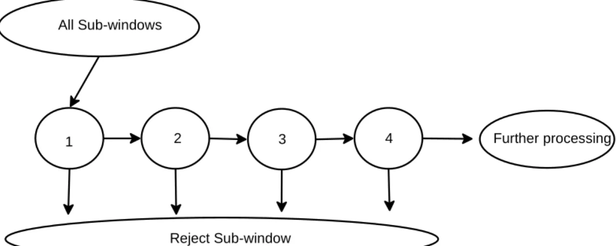
The scheme of the classifier cascade can be found on the figure 3. The main idea of the detection cascade is that smaller, and therefore more efficient, boosted classifiers can reject many of the background sub-windows while keeping almost all face sub-windows. This is achieved by adjusting the threshold of the boosted classifier so that the false negative rate is close to zero. The cascade is in principle a degenerated decision tree where, in each node, is decided if the sample
probably belongs to background or further information is necessary to classify it. The positive result form one cascade stage triggers the evaluation of consequent classifier. This approach benefits from the fact that in detection task the overwhelming majority of sub-windows belongs to background, thus the classification speed depends almost only on the average classification time for background samples.
The cascade is trained using bootstrapping – the subsequent classifiers are trained using only those training samples which pass through all of the previous stages. This allows the training process to effectively and precisely estimate the weak hypotheses even on the very hard and extremely rare examples which pass to the final stages of the cascade. The bootstrapping requires enormous supply of background samples as the rejection ratio in the later stages can reach 1:1000 and less.
One of the disadvantages of the detection cascade is that the results of previous stages are discarded, even thou they can provide relatively good prediction on the samples which pass the stage. This results in longer classifiers in the later stages then would be possible to achieve if this information was used. This fact was addressed by Xiao at al. [9]. In their boosting chain they use the classifier of previous stage as the first weak hypotheses of current classifier.
1 2 3 4
Reject Sub-window
Further processing All Sub-windows
Figure 3: The detection cascade of boosted classifiers.
2.5.2
WaldBoost
Šochman and Matas in their WaldBoost algorithm [37] combine AdaBoost with Wald’s sequential probability ratio test which solves the problem of creating optimal classification strategy in terms of the shortest average decision time subject to a constraint on error rates. WaldBoost classifier is almost identical to the AdaBoost classifier, except each weak hypothesis can be assigned two (for each class) early termination thresholds. If the strong classifier sum exceeds one of these thresholds, the sample is classified to corresponding class, otherwise the evaluation of the classifier continues. The termination thresholds are selected to achieve desired false positive and false negative rates. The classifier is trained with bootstrapping as in the case of cascaded classifiers. This implies that in detection tasks, only thresholds for rejecting background samples are used, as it is usually not
possible to get more face examples. The authors note that they use independent validation set to select the thresholds.
2.6
Learning Speedup
As noted in section 2.3, the computational complexity of the AdaBoost learning algorithm in the detection tasks is θ
(
N⋅M⋅T)
where N represents the number of examples, M represents the number of the features and T is the number of algorithm iterations. Although the computational complexity seams reasonable, the learning time may still reach many ours or even days in cases with high number of samples or many weak hypotheses to choose form. Although this may not be a problem when creating new classifiers for particular practical applications, it may significantly constrain the possibilities of experimenting with new variations of learning algorithms and features.One way to reduce the learning time, which was proposed by Friedman et. al [38], is to use only a fraction of examples in each iteration which have currently the highest weights. This approach has its justification in the fact that samples with higher weights influence the result more then those with low weights. Therefore it is reasonable to use the available computational power on the samples with higher weights. The suggested size of the fraction of samples used is between 0.99 and 0.9 of the total weight mass. This approach does not reduce the performance of resulting strong classifier much; however, it shifts the distribution over the examples. This may be solved by resampling which eliminates some of the samples with low weights and appropriately raises weights for other samples with originally low weights.
3
Data Transformations in Computer
Vision
One of the important tasks in classification is to extract a set of suitable features from the available data. The features should have high classification-related information content compared to the data in its original form to enable the machine learning algorithms to achieve better results. The transformation of the original data, obviously, does not add any additional information, but it can make the relevant information much easier to be found by the learning algorithm. In general case, linear transforms, such as principal component analysis (PCA) or linear discriminant analysis (LDA), can be used to extract relevant features. When additional prior knowledge about the data is available, it should also be utilized in the feature generation. In computer vision, the data usually represents two dimensional discrete signals which exhibit strong spatial relations. Some particular knowledge about the structure of the data – about the spatial/frequency relations – can be utilized e.g. by using linear transforms with suitable fixed basis vectors such as Fourier transform, discrete cosine transform (DCT), or wavelet transforms [39]. More specialized features are used in some specific task such as optical character recognition where the image is usually preprocessed and then some features describing shape are extracted.
When using AdaBoost in computer vision problems, it is possible to use highly over-complete set of features based, for example, on some kind of simple wavelets. If the weak hypotheses are simple (e.g. decision stumps1) and each is based on a single feature, then AdaBoost essentially tries to select the most discriminative and, at the same time, compact sub-set of the features. This approach results in higher classification precision and lower number weak hypotheses in the final classifier, then if a classic wavelet transform was used. In the following text, we describe some of the most common data transforms used in computer vision in connection with AdaBoost.
3.1
Haar-like Features
Haar-like features were used in combination with AdadBoost for the first time by Viola and Jones in their face detection system [5]. Since then, many authors continued this work [6] [7] [8] [9] [10] [11] [13] [37]. Also, other applications of these features emerged. For example, in [41] the authors use WaldBoost classifier with Haar-like features as an approximation of Hassian-Laplace detector to detect points of interest in images. The Haar-like features are generally very suitable for detection tasks as they can be computed very fast and in constant time using a structure called integral image
[5]. One disadvantage of Haar-like features and all other features based on wavelets is that they need some normalization to achieve intensity scale invariance. Normalization by standard deviation of intensity of the sample is usually used. This normalization, although simple and effective on CPU, can be problematic on other platforms like GPU and FPGA.
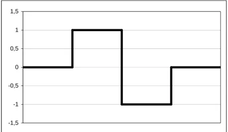
Haar-like features are derived from Haar wavelets which were proposed already in 1909 by Alfred Haar [40]. Note that this was even before the term wavelet was established. The Haar wavelets are the simplest possible wavelets. They are basically a localized step function (see figure 4). The Haar-like features extend the wavelets to 2D and some of them are little bit more complex. The most basic Haar-like features are composed of two adjacent, axis-aligned rectangular areas of equal size. The result is then the difference of the average intensity value in the two areas. Also more complex features exist. Some of the Haar-like features which have been used in practical applications are shown in figure 5. -1,5 -1 -0,5 0 0,5 1 1,5
Figure 5: The Haar-like features which were used in practical applications.
The term integral image was first used by Viola and Jones in [5]; however, similar structure called summed area tables was used earlier in computer graphic. The integral image is an intermediate representation which makes it possible to compute sums of values in arbitrary sized axis-aligned rectangular areas in constant time with only four accesses to memory. The integral image at location
y
x, contains the sum of the pixels above and to the left of x,y, inclusive:
( )
∑
(
)
≤ ≤ = ' , ' ' , ' , y y x x y x i y x iiwhere ii ,
( )
x y is the integral image and i ,( )
x y is the original image. Also some modifications to the integral image exist. In [6], the authors use extended set of Haar-features which use integral image rotated by 45°.3.2
Gabor Features
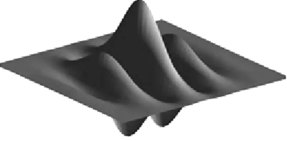
Gabor wavelets [44] are preferred for their higher descriptive power in applications where the computational time in not so critical [42][43]. Gabor wavelets provide ideal trade-off between frequency resolution and spatial resolution. Another interesting motivation for using 2D Gabor wavelets in computer vision is that they are closely related to how the images are processed in the human visual cortex [44]. Gabor function is a Gaussian-modulated complex exponential (see Fig 6). Similarly to the Haar-like features, the Gabor wavelets also need normalization to achieve intensity scale invariance.
Figure 6: The 2D Gabor wavelet.
3.3
Local Binary Patterns
Local Binary Pattern (LBP) is a texture analysis operator which provides information about local texture structure invariant to monotonic changes in gray-scale and possibly to rotations. LBP creates a binary code by thresholding a small circular neighborhood by the value of its center (see Fig 3). The original definition of LBP [45] was extended to arbitrary circular neighborhoods in [46]. Invariance to rotations can be achieved by merging appropriate code values [47]. Rotation invariance can be further improved by distinguishing only uniform patterns [47] – patterns with at most two transitions between 0 and 1 in the corresponding binary code.
LBP operator was used in many practical applications mostly tightly connected to static texture analysis [45][47][48][49] and dynamic texture analysis [50], but also in face recognition[51][52] and authentication [53], facial expression recognition [54] and palmprint identification [54]. For further information on LBP and examples of successful application see [56].
Figure 7: Fig 3: Local binary patterns (LBP) as presented in [54].
3.4
Linear Transforms
Linear transform is a function between two vector spaces that preserves the operations of vector addition and scalar multiplication. When considering finite-dimensional vector spaces, every linear
transformation can be represented as a matrix multiplication. When considering the use of linear transforms in classification applications, they can be used to reduce the data dimensionality, they can transform the data to a vector space where the distinct classes can be easily separated and/or they can provide a way how to utilize some knowledge about the data.
Linear transforms have many uses in the field of computer vision and image processing. Probably the most widely used linear transform in image processing is the discrete Fourier transform (DFT), which transforms the original two dimensional image signal into a discrete spectrum of its frequency components. The basis vectors of the discrete Fourier transform are complex exponentials with rising frequency. It may be beneficial to use DFT to transform images before classification, as DFT decorrelates the original data using our knowledge about some inherent structure of the data. For practical classification application, it is more suitable to use the discrete cosine transform (DCT) which provides real-valued results. Except these two transformations, many other exist. Also wavelet transformations are linear.
Many general linear transforms are used to support classification such as principle component analysis (PCA), linear discriminant analysis (LDA) and independent component analysis (IDA), etc. These transforms do not have fixed basis vectors as in the case of DFT and DCT, but the basis vectors are rather estimated from the data based on some objective criteria. In PCA, the bases vectors are computed in such way that the first one reflects the direction of the largest variability in the original data and this variability decreases for further bases vectors. For example, in [10], the authors use a cascade of AdaBoost classifiers where the first stages use Haar-like features and the later stages use features derived from PCA. This approach is beneficial, since the PCA features offer enough discriminative power even in the later stages of the cascade where the Haar-like features are too weak to discriminate the hard examples. On the other hand, the PCA features are too computationally expensive to be used in the first stages of the cascade. This way, the cascade preserves the high classification speed while increasing its accuracy. LDA is related to PCA, but, in this case, the bases vectors represent directions in which samples from different classes can be best separated. The goal of ICA is to find such linear transform of non-gaussian data so that the resulting features are statistically independent, or as independent as possible.
4
Weak Learning Algorithms
Weak learning algorithm in the context of PAC learning framework is any learning algorithm which can achieve at least slightly better results then random guessing on arbitrary distribution over the training samples. Although the weak learning algorithms which can be boosted by AdaBoost are not restricted in any other way, in practice, only very simple weak learners are usually used. The commonly used weak learners include histograms, decision stumps and decision trees. All of these weak learners are members of a group of so-called domain-partitioning weak hypotheses1 and use only single feature to form their prediction. The domain-partitioning weak hypotheses divide the feature space Χ into disjoint blocks which cover all of X and the prediction values of the hypotheses depend only on which block a sample falls into.
Some work has been also done to explore the possibilities of using more complex weak learners such as artificial neural networks and SVM. However, these weak learners are not widely used.
There are two main reasons to use simple weak learning algorithms. The first reason, which is most relevant in real-time applications, is the low computational complexity of such algorithms. The simple weak hypotheses are very fast and more complex hypotheses do not usually provide adequate speed-up to justify their computational cost. In this context it is more effective to use some data transformation technique (Haar-like features, PCA, …) then to use more complex classifiers. The second reason is connected with generalization properties of the strong classifier, as it is not fully clear how the boosting algorithms will perform with such complex hypotheses.
4.1
Histograms
Histograms are the simplest weak classifiers. When considering only histograms based on single feature, the partition blocks are formed by equidistant hyper planes which are perpendicular to one of the dimensions of the feature space. In other words, this is equal to dividing the real line of the possible feature values into connected intervals which have equal width. In further text, we will call such partition blocks which are based on single feature bins.
As noted in [57], these weak learners are still used by many authors [58] [59], although they suffer from many drawbacks. The first drawback is that there is no general rule how to set the number of bins. The appropriate number of bins is usually chosen according to experiments. Another drawback is that the bins are, in every, case far from optimal. In areas where the probability distribution functions change rapidly, the equidistant bins are not able to capture the rapid changes.
On the other hand, in stable regions the number of bins is unnecessarily high and reduces the prediction power of the weak hypothesis due to the smoothing coefficient (5).
4.2
Decision Trees and Decision Stumps
These weak hypotheses eliminate the main drawback of the histograms which are the fixed bin boundaries. The decision stumps were historically the first weak hypotheses used with AdaBoost, because they are suitable for discrete AdaBoost as they inherently divide the samples into two bins. The decision stumps have been also used in many successful practical applications [5][6][11]. A decision stump can be viewed as a degenerated decision tree with only the root node and two leaf nodes. As such, the decision stumps contain only single threshold which divides the samples into two bins.
The weak learner’s task in the case of decision stumps is to find suitable position for the threshold. The threshold should be set to such position which assures the best classification performance of the resulting hypothesis. In the case of discrete AdaBoost, weighted classification error (1) was used as the criteria to place the threshold. In real AdaBoost, the optimal criteria is the minimization of the Z value (4). t
The decision trees are basically recursive decision stumps. They perform greedy optimization of some criteria. Again, the optimal criteria which assures the fastest minimization of the bound on the training error is based on the Z value. Some authors, however, propose different optimization t
criteria. For example, in [57] the authors use criteria based on entropy and select the best weak hypothesis based on Kullback-Liebler divergence. In the case of decision, the number of leaf nodes needs to be somehow controlled. There is the possibility to explicitly restrict the depth of the tree or the number of nodes. It is also possible to define some stopping criteria. Such criteria was used in [57]. In real applications, the need to limit the number of leaf nodes does not pose a problem, because even very low number of leaf nodes is sufficient (6-20) to achieve best possible performance and in such case the smoothing coefficient does not significantly weaken the predictions.
As noted in the previous text, the decision trees perform a greedy minimization. The problem of finding optimal bins can be, however, solved more precisely. For example, it is possible to use dynamic programming to find the optimal thresholds.
5
New Image Features
In this section, we present newly developed image features which are suitable for implementation of object detection classifiers in FPGA.
The contemporary state of the art real-time object detection classifiers are modifications of cascade1 of boosted2 decision trees or decision stumps3 based on Haar-like features4. Such classifiers benefit from the effective computation of the Haar-like features which takes constant time for all sizes of the features. This allows scanning sub-windows of different sizes without the need to scale the image (the classifier is scaled instead). An intermediate image representation called integral image is used for evaluation of the features. This integral image is also used to efficiently compute standard deviation of pixel values in the classified area, which is used to normalize the features. Another reason why these classifiers are so fast is that the weak hypotheses (histograms, decision trees or decision stumps) are very simple and fast. Finally, the cascaded classifiers make early decisions for most of the background image areas and thus reduce the mean number of weak classifiers which need to evaluate (to 5-20 weak classifiers). All of these facts enable the classifier to scan all the sub-windows needed to reliably find the object even in high-resolution video. To sum it up, the speed of the classifier depends on how fast the weak classifiers are computed and how much discriminative power they offer. The demand for high discriminative power arises from the fact that higher discriminative power of the weak classifiers implies lower average number of evaluated weak hypotheses needed to make reliable classification decision.
The classifiers discussed in the previous text are optimized for general purpose CPUs which can not be used in many applications due to high power consumption, high cost and/or space limitations. Such applications include, for example, digital cameras, camcorders, surveillance, traffic monitoring and mobile robots. The solution for such applications can offer programmable hardware – FPGA. In contrast to the CPUs, FPGAs offer better energy consumption – computational power ratio, but only if the algorithms can suitably parallelized and mapped to the device. The limitations of FPGAs include limited numerical precision, low local memory capacity and limited resources for the algorithm itself.
The classic boosted classifiers based on Haar-features are not much suitable for implementation in FPGA for number of reasons. First, relatively high precision is needed for the integral image (16-18b for features 32x32 pixels large) and the access to the integral image is absolutely random.
1 See section 2.5 for more information. 2 See section 2.2 for more information. 3 See section 4.2 for more information. 4 See section 3.1 for more information.
![Figure 1: The original version of AdaBoost[2] with notation modified according to [26]](https://thumb-us.123doks.com/thumbv2/123dok_us/9229188.2807481/18.892.117.798.155.873/figure-original-version-adaboost-notation-modified-according.webp)
![Figure 2: The totally corrective step [7].](https://thumb-us.123doks.com/thumbv2/123dok_us/9229188.2807481/23.892.117.807.445.787/figure-totally-corrective-step.webp)


![Figure 11: A simplified diagram of the FPGA engine for evaluation of the LRD as presented in [17]](https://thumb-us.123doks.com/thumbv2/123dok_us/9229188.2807481/38.892.119.751.633.980/figure-simplified-diagram-fpga-engine-evaluation-lrd-presented.webp)