c
ITEM SELECTION METHODS IN POLYTOMOUS
COMPUTERIZED ADAPTIVE TESTING
BY
USAMA SAYED AHMED ALI
DISSERTATION
Submitted in partial fulfillment of the requirements
for the degree of Doctor of Philosophy in Educational Psychology in the Graduate College of the
University of Illinois at Urbana-Champaign, 2011
Urbana, Illinois Doctoral Committee:
Professor Carolyn J. Anderson, Chair
Professor Hua-Hua Chang, Director of Research Professor Jeffery Douglas
Abstract
Given the rapid advancement of computer technology, the importance of administering adaptive tests with polytomous items is in great need. With regard to the applicability of adaptive testing using polytomous IRT models, adaptive testing can use polytomous items of either rating scales, or in some testing situations of multiple choice. Additionally, the availability of computerized polytomous scoring of open-ended items enhances such applicability. This need promotes the research in polytomous adaptive testing (PAT). This dissertation is an effort to focus on item selection methods, as a major component, in polytomous computerized adaptive testing. So, it consists of five chapters that cover the following:
Chapter 1 focuses on a thorough introduction to the item response theory (IRT) models and adaptive testing related to polytomous items. Such an important overview and introduction to basic concepts in test theory and mathematical models for
polytomous items is needed for the flow of consequent chapters. Chapter 2 is devoted to the development of a central location index (LI) to uniquely represent the polytomous item with a scale value parameter using most commonly used polytomous models. The motivation and rationale to search for a central or an overall location parameter is twofold: a) the confusion of multiple and different parameterizations for a polytomous item even for the same model, and b) the unavailability of such single location parameter block the usage of certain item selection methods in adaptive testing. Two approaches are used to derive the proposed LIs, one is based on the item category response functions (ICRFs) and the other is based on the polytomous item response function (IRF). As a result, four LIs are proposed. Chapter 3 is particularly assigned to development of an item selection method based on the developed location index and primarily assess its performance in the PAT context relative to existing methods. This method belongs to the non-information based item selection methods and we referred it as Matching-LI method. The results support that this proposed method is promising and is capable to produce accurate ability estimates and successfully manage the item pool usage. Chapter 4 introduces new item selection methods taking in consideration the previous chapter’s results. The new methods are the hybrid, stage-based information, polytomous a-stratification methods.
The first two methods try to merge more than one criterion for selecting items of each PAT (e.g., the hybrid method merges both the Matching-LI and maximum information (MI) methods). The last method uses Matching-LI method within each stratum. Chapter 5 provides discussion, conclusions, and limitations and future research directions with respect to important components of an adaptive testing program (i.e., item selection methods, item response models, item banks, and trait versus attribute estimation).
Acknowledgments
First and foremost, all my gratitude is due to God Almighty for guiding me through, and aiding me in completing this work. Then, I would like to give thanks to my family, especially my parents for their support, encouragement, and advice. I would also like to give my sincere thanks to my advisor Professor Hua–Hua Chang who provided me with technical experience in educational measurement research and life skills. I really
appreciate his persistence in advising to uplift my performance and to hasten to the top. I would like to give my gratitude to Professor Carolyn Anderson who passionately helped me to her best in different aspects. I really appreciate her great efforts toward furthering my career.
Much gratitude to Professor Jeffery Douglas and Professor Jinming Zhang for serving as committee members, and constantly being there for me. I would like to thank two of my colleagues Chia-Yi Chiu and Aaron Oaks for their endless technical support.
Also I would like to thank the Egyptian Government, the Ministry of Higher Education, and the Egyptian Cultural and Educational Bureau in Washington D.C. that supported me for four years to fulfill my mission here in the States.
Finally, I do appreciated the great role of my wife who stood besides me to attain such position. I ask Allah to help and reward her, and all who have a right on me, the best and guide us to please Him.
Table of Contents
List of Tables . . . vii List of Figures . . . viii Chapter 1 Polytomous Item Response Models and Adaptive
Testing . . . 1 Chapter 2 Development of Location Indices for Polytomous Items
and Their IRT Applications . . . 17 Chapter 3 Matching Location Index as a Non-information Item
Selection Approach in Polytomous Adaptive Testing . . . 30 Chapter 4 Improving the Performance of
Matching-Location-Index Method With Information Indices . . . 45 Chapter 5 Discussion and Conclusion . . . 61 References . . . 66 Appendix A Approximation of LIIRF Value Using Newton-Raphson
Method . . . 70 Appendix B IRT Parameters and Information Curves of 93 NAEP
List of Tables
1 Studied ICRFs and Corresponding Intersection Points. . . 21 2 Item Parameters and the Corresponding Location Indices (LIs). . . 28
3 Descriptive Statistics of Simulated Item Pool (No Reversals). . . 36 4 Overall Measurement Precision Indices Under Different Item
Selection Methods (N=1000, M= 300, L=15). . . 39 5 Conditional Bias and MSE Under Different Item Selection
Methods (N=1000, M= 300, L=15). . . 40 6 Overall Item Pool Usage Indices Under Different Item
Selection Methods (N=1000, M= 300, L=15). . . 41 7 Percentages of Exposure Rates for Over-exposed Items
(N=1000, M= 300, L=15). . . 42
8 Descriptive Statistics of Real Item Pool (M=93). . . 54 9 Measurement Accuracy Indices for Different Item Selection
Methods (N=1000, M= 93, L=9) . . . 57 10 Descriptive Statistics of Pool Utilization by Different Item
Selection Methods. . . 58 11 Item Utilization Indices andMostly Selected Items by
Different Item Selection Methods . . . 59
List of Figures
1 Item and category KL information curves (θ0 = 0).. . . 13
2 Item and category KL information curves (θ0 =−1).. . . 13
3 Item information and expected score curves for a 3-category item. . . 15
4 Item category characteristic curves (ICCCs) for a 3-category item.. . . 22
5 Item category characteristic curves (ICCCs) for a 5-category item.. . . 23
6 Item characteristic curve (ICC) for a 3-category item. . . 25
7 Item characteristic curve (ICC) for a 5-category item. . . 26
8 Item category characteristic curves (ICCCs) for a 2-category item.. . . 27
9 Expected score curve for a 2-category item.. . . 28
10 Distribution of a-parameter and LIs for all items in the item pool. . . 37
11 Distribution of LIs for all items in the item pool. . . 38
12 Distribution of item exposure rates of the item selection methods. . . 42
13 Relationship of LImean and LIIRF with discrimination parameters.. . . 55
14 Total item bank information.. . . 56
B1 Information functions for items 1-24 . . . 75
B3 Information functions for items 49-72. . . 77 B4 Information functions for items 73-93. . . 78
Chapter 1
Polytomous Item Response Models and Adaptive Testing
The current chapter provides an important overview and introduction to basic concepts in test theory and mathematical models for polytomous items. This is required to understand the proposed methods for item selection in computerized adaptive testing for polytomous items that are described and studied in this dissertation.
Introduction
Item response theory (IRT) is critical to large-scale assessment, and computerized adaptive testing (CAT) is considered one of the major modern developments of IRT. Until recently, most of the research and applications of CAT focused on dichotomous items, and only a few studies have investigated CAT with polytomous items and more specifically polytomous item selection methods (Choi & Swartz, 2009; Dodd, De Ayala, & Koch, 1995; van Rijn, Eggen, Hemker, & Sanders, 2002). The polytomous items are important for various testing purposes such as education, personality, attitudes and more (Embretson & Reise, 2000).
Both dichotomous and polytomous items are used in many standardized tests such as state assessment measures. In addition, tests consisting of polytomous items are
preferable for one or more of the following reasons: (a) fewer polytomous items can attain the same reliability compared to the dichotomous items, (b) the easiness of assessing some traits using rating scales, and (c) the suitability of expressing item responses on an ordinal scale (van der Ark, 2001).
Different models are available for modeling polytomous item responses. Examples of such models are: the graded response model (GRM; Samejima, 1969), the nominal response model (NRM; Bock, 1972), the partial credit model (PCM; Masters, 1982), and the generalized PCM (GPCM; Muraki, 1992). The current study focuses on the work related to the polytomous adaptive (PAT) system. Basically as in dichotomous CAT, PAT consists mainly of four components (e.g., Dodd et al., 1995; Lima Passos, Berger, & Tan, 2007):
2. Item selection method. 3. Ability estimation procedure. 4. Stopping rule.
The first component in CAT is the pool of items that is used as a resource to deliver adaptive tests. In dichotomous CAT, the item pool needs to contain enough number of items to satisfy the purpose of testing (Lord & Novick, 1968). On the other hand, an item bank composed of 30 polytomous items was considered sufficient to successfully estimate the ability or trait level in PAT. This result did not take into consideration the security of item banks in terms of item exposure rate, or the issue of content balancing. In addition, the distribution of item bank information is another problematic issue, such as skewed or bimodal distributions (Dodd et al., 1995). Therefore, a larger item bank is required to deal with these issues.
The second critical component in adaptive testing to efficiently utilize the item pool to sequentially select item after item depending on the examinee’s current ability estimate (i.e., ˆθ) until the end of test. This dissertation focuses on new item selection rules for polytomous items.
The third issue in PAT is ability (or latent trait) estimation approaches. In the literature, they can be classified into frequentist and Bayesian methods. Maximum likelihood estimation (MLE) is a popular estimation method belonging to the first category. Bayes modal (BM), maximum a posteriori (MAP), and expected a posteriori (EAP) are Bayesian estimators used in CAT. Here we need to mention that ability estimation procedures are under continuous development. Tao, Shi and Chang (2009) proposed a new version of MLE to include scoring weights, called item-weighted likelihood estimator (IWLE), into the process of estimation. That IWLE method is different from Warm’s (1989) weighted likelihood estimation method.
The final component of a CAT algorithm is a stopping rule that terminates the test. Different termination criteria to end a test exist. One approach is to administer a fixed number of items. This approach is called fixed-length adaptive testing and it is preferable in situations where the number of delivered items is a concern. Another
approach that is used as a stopping rule is whether a predetermined measurement
precision has been achieved. The administration of items will continue until the standard error of measurement is below an acceptable value (Embretson & Reise, 2000). The latter approach is called variable-length adaptive testing. A third approach is to terminate the test after a predetermined time is elapsed. A mixture of these approaches can be
practically used as well such as using both target precision and maximum number items a stopping rule.
Toward the enhancement of PAT, the development and enhancement of item selection criteria is our starting point.
The dissertation consists of five chapters: (a) the first chapter focuses on an thorough introduction to the IRT models and adaptive testing related polytomous items, (b) the second chapter is devoted to the development of a central location index to uniquely represent the polytomous item with a scale value parameter using most commonly used polytomous models, (c) the third chapter is particularly assigned to development of an item selection method based on the developed location index and primarily assess its performance in the PAT context relative to existing methods, (d) the fourth chapter introduces new item selection methods taking in consideration the previous chapter’s results, and (e) the fifth chapter provides discussion, conclusions, and limitations and future research directions.
The reminder of this chapter covers different mathematical IRT models of polytomous items, the connection among them, and the parameters describing item properties, followed by explaining two item information measures, other modifications applied to the original measures, and their relation to item selection criteria. Then, the chapter concludes with defining the key terms used through out the research.
Polytomous IRT Models
Test items that have more than two response categories are called
polytomously-scored items. Both dichotomously and polytomously-scored items are ubiquitous in educational and psychological testing. Due to the different scoring scheme, polytomous IRT models should be used in item parameter calibration and ability
In the dichotomous item case, the test administrator classifies the observed responses into one of two categories, correct or incorrect. This dichotomization treats all incorrect answers as equivalent to one another. As such all the mathematical operations required to answer an item on a mathematics test are considered una voce (i.e., as a “single operation”). If an examinee correctly performs all the operations and their response is categorized as a correct response, they receive a value of 1. Otherwise, the response is categorized in the incorrect category with assigned value of 0. The value assigned to responses reflects only whether the examinee has correctly performed (heuristically) one “operation” (De Ayala, 2009).
In contrast, consider the following mathematical test item as an illustration:
(6/3) + 2 =?.
A scoring rubric for this item might be based on the operations or subtasks needed to answer this item correctly. Therefore, for this itemithere exist three possible integer scores xi for this item, xi= 0,1,or 2. These scores are called category scores that might
indicate the number of successfully completed operations. In general, polytomous test items are scored in a way that reflects a particular score category out ofm+ 1 scores (i.e., x= 0,1, ..., m) that an examinee has achieved, been classified into, or endorsed. Examples of this includes the case where a person gets a score of 2 on an item that is scored from 0 to 4 or a person selects a “disagree” option on a 5-point Likert-scale item (De Ayala, 2009; Ostini & Nering, 2010).
With regard to the applicability of adaptive testing using polytomous IRT models, CAT can use polytomous items of either rating scales, or in some testing situations of multiple choice (Wang & Wang, 2001). Additionally, the availability of computerized polytomous scoring of open-ended items enhances such applicability as suggested by Bennet, Steffen, Singley, Morely, & Jacquemin’s (1997) research.
For the purpose of modeling polytomous data, polytomous IRT models were proposed. One classification of the polytomous IRT models is in terms of whether the category responses are treated as nominal and ordinal variables. In another classification
scheme, polytomous IRT models fall in one of two main categories based on the
mathematical form of the model (Thissen & Steinberg, 1986). One category consists of
differencemodels such as Samejima’s graded response model (GRM; Samejima, 1969), and the other consists of divided-by-total models such as the nominal response model (NRM; Bock, 1972). For ordinal polytomous models, Mellenbergh (1995) defined different classification scheme in terms of the models’ different order-preserving mechanisms in forming the dichotomies of response categories. He classified them into three classes:
1. the cumulative probability (or graded-response) models. 2. continuation ratios (or sequential) models.
3. the adjacent-category (or partial-credit) models.
In the following subsections, a brief description of each model of the most commonly used models, its parameterization, the meaning of the models’ parameters, and relationships among these models are provided.
Nominal response model. For nominal item responses, Bock (1972) proposed that the probability of responsex to an itemiby an examinee with abilityθ, denoted by Pix(θ), equals Pix(θ) = exp(cix+aixθ) Pm x=0exp(cix+aixθ) , x= 0, 1, . . . , m, (1) whereaix is a slope (analog to discrimination) parameter of categoryx,cix is a location
(analog to difficulty) parameter of category x, and m+ 1 is the number of response categories to item i.
For model identification, either sums are set to zero (i.e.,P
aix =Pcix = 0), or
one response category is set to to zero (e.g., the parameters of the lowest response category,ai0 =ci0 = 0). For simplicity, there is no examinee subscript on the ability parameterθ in the current and subsequent models. For each category of an item, there exists an item category response function (ICRF), and the set of ICRFs per item is uniquely determined given a set of identification constraints. Figure 1 provides the item category characteristic curves (ICCCs) obtained from the ICRFs of a 4-category item; one ICCC corresponds to an ICRF. At each level on the ability continuum, the sum of ICRFs
equals 1 (i.e., Pm
x=0Pix(θ=θ0) = 1).
Bock’s NRM is a general polytomous model that is used for mutually exclusive response categories. Item response categories are not necessarily ordered and the NRM is the only model for nominal categories. Mellenbergh (1995) has showed that the NRM can be reformulated in terms ofm log odds for a nominal variable of (m+ 1)-response
categories. He treated them asm dichotomous response variables that correspond to choices of m categories to a reference category. The log odds of choosing a score category x over the first category is as follows:
ln Pix(θ)/ Pi0(θ) = ln exp(cix+aixθ) exp(ci0+ai0θ) = (cix−ci0) + (aix−ai0)θ= (cix+aixθ), x= 0,1, . . . , m. (2)
Ifm= 1 (i.e., dichotomous item), then the NRM reduces to the two-parameter logistic model, where the probability of answering the item correctly, Pi(θ) =Pi1(θ) and the
probability of answering the item incorrectly,Qi(θ) = 1−Pi1(θ) =Pi0(θ). This can be described by ln Pi(θ)/ 1−Pi(θ) = ln Pi1(θ)/ Pi0(θ) = (ci1−ci0) + (ai1−ai0)θ= (ci1+ai1θ), (3)
and the parameters of the reduced model areai =ai1,bi =−ci1/ai1.
Graded response model. Samejima (1969) proposed a model for items with ordinal response categories (e.g., Likert-scale items). Samejima’s graded response model (GRM) is one of the difference models (Thissen & Steinberg, 1986); even Samejima is against such categorization and her model can be expressed as a divide-by-total model (Samejima, 2010). The GRM expresses the cumulative probability of getting at least a scorex on itemi
Pi∗(X≥x) =Pix∗ = exp(ai(θ−bix)) 1 + exp(ai(θ−bix))
wherex= 1,2, . . . , m, and therefore the probability of responding in a specific category score isPix =Pix∗ −Pi,x∗ +1. Note that it is assumed in GRM thatPi∗0 = 1 and Pi,m∗ +1 = 0.
Also, the bivs are ordered such as bi1 < bi2 < . . . < bim.
Partial credit model. Masters (1982) developed a polytomous model, the partial credit model (PCM), that is different in terms of its parameterization and conceptualization from the GRM. This model is an extension of the dichotomous Rasch model. The PCM belongs to the adjacent-category models in Mellenbergh’s classification of IRT models, and to the divide-by-total models in Thissen and Steinberg’s classification. Items are viewed as requiring multiple steps to obtain a correct answer. Incorrect response options reflect partial knowledge; therefore, partial credit is given to each step completed. For an examinee with ability θ, the probability of selecting category or response optionx of item i, denoted byPix(θ), equals
Pix(θ) = expPx v=1(θ−biv) 1 +Pm c=1exp Pc v=1(θ−biv) , (5)
wherebiv is an item-category location parameter. For notational convenience,
P0
v=0(θ−biv) = 0. The location parameterbiv can be broken down into an item location
parameter (i.e., bi ), and a category threshold (i.e.,div) such thatbiv=bi−div. The
difference in ability levels between two adjacent categories, xand (x+ 1), is called the step difficulty or threshold,dix. The log odds based on the PCM equals
lnPix(θ)/
Pi,x−1(θ)
= (θ−bix), x= 0,1, . . . , m. (6)
In the PCM, the thresholds need not to be ordered; harder steps may be preceded by easier steps and vice versa.
Generalized partial credit model. As noticed above the PCM is based on the Rasch model and considers items to be equally discriminating. Relaxing this assumption and allowing items to be differentially discriminating led to the invention of the
generalized partial credit model (GPCM; Muraki, 1992, 1993). The ICRFs of GPCM can be written as
Pix(θ) = expPx v=1Ziv(θ) 1 +Pm c=1exp Pc v=1Ziv(θ) , (7) and Ziv(θ) =Dai(θ−biv) =Dai(θ−bi+dv), (8)
whereD is a scaling constant that puts the trait scale in the same metric as the normal ogive model (D= 1.7) or stays on the metric of the logistic model (D= 1), ai is a slope
parameter for item i,biv is an item-category parameter, bi is an item location parameter,
and dv is a category parameter. Ifm= 1, the model reduces to Birnbaums (1968)
two-parameter logistic model. If all ai are equal, the GPCM reduces to the PCM. These
two restrictions combined yield a polytomous Rasch model. The log odds based on the GPCM is
lnPix(θ)/
Pi,x−1(θ)
=ai(θ−bix), x= 0,1, . . . , m. (9)
Without assuming the order of response categories the log-odds in Equation 2, following the NRM log odds, can be expressed as
lnPix(θ)/ Pi,x−1(θ) = ln exp(cix+aixθ)
exp(ci,x−1+ai,x−1θ)
= (cix−ci,x−1) + (aix−ai,x−1)θ,
x= 0,1, . . . , m. (10)
Constraints can be replaced on parameters of the NRM such that it is a GPCM, specifically, (cix−ci0) + (aix−ai0)θ must equal ai(θ−bix). Therefore, the relationship
between parameters in the NRM and GPCM can be expressed as
ai= (aix−ai,x−1) and bix =−
(cix−ci,x−1)
(aix−ai,x−1)
(11) Both the PCM and GPCM contain a similar term Zix+(θ) (i.e., the sum ofZiv(θ)).
Zix+(θ) = x X v=1 Ziv(θ) = x X v=1 Dai(θ−bi+dv) =Dai " x(θ−bi) + x X v=1 dv # , (12)
and can be rewritten as
Zix+(θ) =Dai[Tx(θ−bi) +Xx]. (13)
Andrich (1978) calledTx the scoring function and Xx the category coefficient. Information Indices and Related Item Selection Rules
In this section, information functions for polytomously scored items are presented. These information indices are very important; because item selection methods were built using them. Examples of such information-based item selection criteria are: maximum information criterion and maximum Kullback-Leibler information criterion. Subsequently more sophisticated versions of item selection rules based on Fisher and Kullback-Leibler information indices are described.
Fisher and observed information. The observed information is given by,
J(θ) =− ∂2logL ∂θ2 , (14)
whereLis the likelihood of a sample of nindependent item response observations (van der Linden & Pashley, 2000). A well known index in statistics is Fisher information that gives the amount of information provided by data on an unknown parameter, θ. It is given by,
I(θ) =−E ∂2logL ∂θ2 =E(J(θ)), (15)
whereE is the expectation to be found with respect to the responses. These two information measures are equivalent under dichotomous IRT models (van der Linden, 1998). Also, they are the same under the GPCM (Donoghue, 1994; Muraki, 1993). However, this equality is not satisfied under other models such as GRM with items of three or more response categories. This was the reason for Choi and Swartz (2009) to investigate the performance of some Bayesian item selection methods based on these two
measures under GRM.
Bock (1972) introduced the information due to the responses in category xas a partition of the item information, and Dodd et al. (1995) provided the general formula of the item information function (IIF) derived from a model for a polytomous item,
Ii(θ) = m X x=0 (Pix0 (θ))2 Pix(θ) = m X x=0 Iix(θ), (16)
wherePix0 (θ) is the first derivative of the probability of getting a scorex on the ith item, Pix(θ), with respect to θ. Iix(θ) is the item category information function and it is clear
that additivity feature is applied to item information over the item categories.
Under the IRT assumption of local independence, the test information function has its additive property across a group of nitems as well, Ii(θ) =
Pm
x=0Iix(θ), (Lord &
Novick, 1968). The factors that affect the item information are complex in polytomous items. For that reason, Akkermans and Muraki (1997) investigated the peaks of the IIF for trinary items (i.e., three-category items).
For a more specific formula of the polytomous item information functions, the above equation can be applied to any model. For the NRM, the IIF, Ii(θ), is given by,
Ii(θ) = m X x=1 a2ixPix(θ)− m X x=1 aixPix(θ) !2 , (17)
whereaix is the item category discrimination parameter (Lima Passos et al., 2007). For
the GRM, the IIF,Ii(θ), is given by (Ostini & Nering, 2010), (Refer to Lima Passos,
Berger, and Tan (2008) for the IIF for the GRM item.)
Ii(θ) = m
X
x=1
Aix. (18)
In Equation 19,Aix is described as the basic function that is given by
Aix=D2a2i
h
Pix∗(θ)(1−Pix∗(θ))−Pi,x∗ +1(θ)(1−Pi,x∗ +1(θ))i Pix(θ)
Under the GPCM, the IIF, Ii(θ), is given by, Ii(θ) =a2i m X x=1 x2Pix(θ)− m X x=1 x Pix(θ) !2 =a2i var(Xi), (20) where thePm x=1x2Pix(θ)−(Pmx=1x Pix(θ))2
is the variance of score on the item given a specific level of ability (Donoghue, 1994). When PCM is considered, the discrimination parameter, ai, is dropped from the above Equation. The Fisher information function is
considered a local index that conveys the information around a single θvalue (Chang & Ying, 1996; Chen, Ankenmann, & Chang, 2000). De Ayala (1992) found that using the category information instead of item information for item selection reduced the test length on average by one item for NRM CAT simulations.
Kullback-Leibler information. In the context of educational testing, Chang and Ying (1996) presented the Kullback-Leibler (KL) information function as a global information criterion for item selection in dichotomous CAT. The KL information function is defined by KLi(θkθ0) =Pi(θ0) log Pi(θ0) Pi(θ) + (1−Pi(θ0)) log 1−Pi(θ0) 1−Pi(θ) , (21)
whereθ0 represents a true ability level andPi(.) is probability of answering item i
correctly. Chang and Ying (1996) mentioned several important features of the KL function:
1. It is not symmetric; that is,KLi(θkθ0)6=KLi(θ0 kθ). 2. KLi(θkθ0)≥0 andKLi(θ0kθ0) = 0.
3. Similar to the additive property of Fisher information, test information is the sum (overn items) of the item information; that is,
KL(n)(θkθ0) =
n
X
i=1
KLi(θkθ0). (22) Note thatKLi(θkθ0) is a function of two variables,θand θ0. Geometrically, the
KL information function is a surface in three-dimensional space, as opposed to a function in two-dimensional space represented by Ii(θ).
As a function of twoθ levels,KLi(θkθ0) represents the power of an item to discriminate between these two levels. When θ=θ0, the value of KLi(θkθ0) is 0 (i.e., the
item cannot distinguish between examinees at the same level of θ). When θ andθ0 are very different, the value ofKLi(θkθ0) is large (i.e., the item can easily distinguish
between examinees with different θs). In other words, the KL is considered as a warning signal that gives a loud alarm when there is a difference between the two θlevels;
otherwise the alarm will be lower. By contrast,Ii(θ) represents the discrimination power
of an item at a single θ.
The KL information index with respect to a polytomous item of (m+ 1) categories can be generalized to the following
KLi(θkθ0) = m X x=0 Pix(θ0) log Pix(θ0) Pix(θ) , (23)
As in the context of Fisher information, we can get the form of category KL (CKL) information function as followed,
KLix(θkθ0) =Pix(θ0) log Pix(θ0) Pix(θ) . (24)
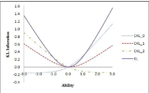
From the graphical representation as shown in Figures 1 and 2, we can see some of the properties of KL and CKL under a given polytomous model, GPCM (note that these curves are part of the KL or CKL surface at a specific level ofθ0, the real ability level),
1. These curves are not symmetric; that is, KLix(θkθ0)6=KLix(θ0 kθ) (e.g., in the graphed item, KLix(θ=−1kθ0 = 0) =.27566=KLix(θ0 = 0kθ=−1) =−.1206. 2. KLi(θkθ0)≥0 andKLi(θ0kθ0) = 0 but KLix(θkθ0) is a real-valued that can
be negative as shown in Figures 1 and 2.
3. All CKL curves and the KL curve intersect at the same point. This point
corresponds to the real ability value; the amount of information of each are equal at that point. For the 3-category item, it is the minimum value of middle-category KL (i.e., the CKL with respect to score 1). In addition, the CKL for first (last) categories is a monotone increasing (decreasing) function, respectively.
Modified information functions. As a step in modifying and refining information functions, Veerkamp and Berger (1997) introduced an interval information
Figure 1: Item and category KL information curves (θ0 = 0).
criterion for dichotomous CAT to overcome the problems of Fisher information. Instead of maximizing Fisher information function at an ability estimate, they proposed to integrate the function over a small interval around the estimate to compensate for the uncertainty in it. In PAT, there is another reason to integrate Fisher information function over an interval. Fisher information function might be multi-modal when items are analyzed with the GPCM (Muraki, 1993). Van Rijn et al. (2002) demonstrated that a multi-peaked item might contain more information for a small interval around the ability estimate than the item that contains maximum Fisher information at the ability estimate. They proposed to select the next item with a maximum interval information criterion:
i= arg max i Z θˆ+δ ˆ θ−δ Ii(θ)dθ, (25)
whereiis a potential item to be administered andδ is a small constant defining the width of the interval.
Other variations of Fisher item information have been proposed and used as alternatives to the original index. The A-optimality or sum criterion, ΦA=PθIi(θ) and
the D-optimality or product criterion is given by ΦD =QθIi(θ) where the distribution of
θis equally weighted within an interval. In general, the A-optimality criterion corresponds to the arithmetic sum and the D-optimality criterion corresponds to the geometric mean (Berger & Veerkamp, 1996). Additional indices such as maximum expected information that depends on the observed information or Fisher information exist.
The relationship between item information and IRF in PAT.The
theoretical relationship between the Fisher information and KL information in the context of polytomous items is still the same as that for dichotomous items. That is, the second derivative of KL information is considered Fisher information at the true ability level.
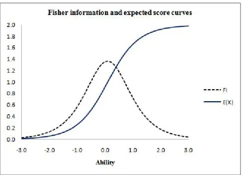
With respect to the relationship between Fisher information function (i.e., Ii(θ)),
and IRF or the expected score (i.e., E[X]). Figure 3 graphically shows the information curve and the polytomous item response function for an item with three categories over the ability continuum.
Figure 3: Item information and expected score curves for a 3-category item.
function, that can also be related to the gradient functionGi(θ) described in Equation 26
as follows, Gi(θ) = ∂T¯i(θ) ∂θ =a 2 i m X x=1 x2Pix(θ)− m X x=1 x Pix(θ) !2 = Ii(θ) ai , (26)
Therefore, the curve of Fisher item information function intersects with the curve of gradient function at the point of maximum information. This is a promising result that could be beneficial and could provide a non-information based item selection algorithm in PAT depends primarily on the polytomous IRF instead of the fisher information as a criterion.
More information in polytomous items. In general, a polytomous item has more information than a dichotomous one. In reality, each pair of the adjacent categories in a polytomous item could be considered as a single dichotomous item (Dodd et al., 1995). For a fixed amount of information, this property makes the required size of the item bank in PAT smaller than its size in dichotomous CAT. In other words, given a dichotomous and polytomous item banks with same number of items the polytomous one contains more information. Also, this may affect the item selection if we have a mixture of
item types, dichotomous and polytomous items. Also, there are some studies that discussed the information in polytomous items under different polytomous IRT models (e.g., Akkermans & Muraki, 1997; Donoghue, 1994).
Definition of Terminology
Below is a summary of terms used frequently through out the following chapters. Polytomous item response model. Item response model for items with more than two response categories (e.g. multiple-choice item that allows partial credits for each of the response categories, or constructed-response item with multiple steps).
Ability estimate. The estimate of the level of a latent trait of an examinee demonstrated by their observed response pattern to a test.
Item response categories. The possible ways as assigned by the item writer that an examinee could respond to an item. In the context of multiple-choice items, item response categories are the options provided for the examinee to choose; in
constructed-response items, they are the steps or parts of the solution to the item that allow different amounts of partial credit to be awarded upon their completion.
Item response function (IRF). The mathematical equation that relates the probability of answering an item correctly as a function of the ability of the examinee attempting the item and the item parameters.
Item category response function (ICRF). The mathematical equation that describes the probability of an item category being chosen as a function of the ability of the examinee and item category parameters.
Item characteristic curve (ICC). The curve that demonstrates the relationship between the ability of an examinee and the probability of the examinee answering the item correctly. Sometimes it is referred as a trace line. It is the graph of IRF plotting against the ability parameters.
Item category characteristic curve (ICCC). The curve represents the relationship between the probability of an examinee choosing an item category and the ability of the examinee. ICCCs of all the categories within an item are usually plotted on the same graph.
Chapter 2
Development of Location Indices for Polytomous Items and Their IRT Applications
The current chapter addresses the need to represent a polytomously-scored item by one index for the use in adaptive testing. Therefore, this chapter introduces the development of location indices for a polytomous item. Possible applications of such indices in CAT are reported as well.
Objective of Study
Items are the building blocks of testing. Based on the scoring of response options, items can be classified into two types: dichotomous and polytomous items. In terms of the parameters that characterize items, they depend on the IRT model that fits such items. For dichotomous items, the two-parameter logistic model are characterized by two properties: an item’s discrimination power (measured by parameter ai for itemi), and
difficulty (measured by parameterbi). In the polytomous case, many polytomous models
use a single discrimination parameter for the item regardless of response option, such as the GRM, PCM, and GPCM. Other IRT models have multiple parameters; one parameter per item category. With regard to item difficulty for polytomous items, models use several parameters or thresholds that depend on item categories; therefore, at least two thresholds will be used to provide an idea of the difficulty for a 3-category item (i.e., scored 0, 1, or 2).
The motivation and rationale to search for a central or an overall location parameter is twofold: a) it may be due the confusion of multiple and different parameterizations for a polytomous item even for the same model, and b) the
unavailability of such a single location index blocks the usage of certain item selection methods in adaptive testing.
Based on the PAT literature, the item selection methods are sometimes natural extensions of those used with dichotomous items, such as information indices. The information-based item selection procedures may consider the item as a whole or at the score category level. Dodd et al. (1995) commented that only the information-based item selection algorithms have been investigated for the GRM, NRM, and PCM because of the
unavailability of a single location index (or scale value parameter).
The potential item selection method to be developed in this dissertation intends to use the properties of item characteristic curve (ICC) and item-category characteristic curves (ICCCs) to define new polytomous item indices.
Item Location Indices
Two general approaches are used to develop item location for polytomous item. The first approach is to study the category response functions and the second one focuses on the item response function. Basically, the proposed indices are based on the ICRFs and IRF of a polytomous item.
The development of such indices given here applies to polytomous models that have the same discrimination across the different item categories where the mathematical derivations introduced here apply for the other models in such category.
Considering the GPCM, the ICRF for scorex on the ith item is
Pix(θ) = expPm v=1ai(θ−biv) 1 +Pm c=1exp Pc v=1ai(θ−biv) . (27)
The definition of model parameters was introduced in Equations 7 and 8.
Studying the item category response functions (ICRFs). Assume a polytomous item with three categories under the GPCM where each category has its own ICRF. The parameters for itemiare: ai,bi1, and bi2. Therefore, we have three ICRFs with the possible scores (0, 1, or 2) on the item,Pi0(θ), Pi1(θ), andPi2(θ). A graphical representation of such a 3-category item is given in Figure 4. This graph provides the rationale behind the following derivations. As seen in Figure 4, the peak of the
partial-credit score curve occurs at the same point that the zero and perfect score curves intersect. It can be shown mathematically that this will always occur for the GPCM. Starting with the probability of attaining the partial credit (middle) score, Pi1(θ), and we
locate the peak of this ICRF. From Equation 1,
Pi1(θ) =
exp [ai(θ−bi1)]
1 + exp [ai(θ−bi1)] + exp [ai(2θ−bi1−bi2)]
and the first derivative of Equation 28 with respect toθ is ∂Pi1(θ) ∂θ =aiPi1(θ)−aiPi1(θ) 2 X c=1 cPic(θ) =aiPi1(θ) " 1− 2 X c=1 cPic(θ) # . (29)
Setting Equation 29 equal to zero, we find that the maximum of Equation 29 occurs when any of the following three conditions hold: ai= 0, Pi1(θ) = 0, or
P2
c=1cPic(θ) = 1 (orE(Xi) = 1). The fist condition, ai = 0, indicates that the item has
no discrimination power, hence, it would not be in an operational item pool. The second condition,Pi1(θ) = 0, is not achievable. All response options have non-zero probability. The third condition, P2
c=1cPic(θ) = 1 or E(Xi) = 1, can be attained as seen by noting
that: 2 X c=1 cPic(θ) = 1 Pi1(θ) + 2Pi2(θ) = 1
exp [ai(θ−bi1)] + 2exp [ai(2θ−bi1−bi2)] = 1 + exp [ai(θ−bi1)] + exp [ai(2θ−bi1−bi2)] exp [ai(2θ−bi1−bi2)] = 1
ai(2θ−bi1−bi2) = 0
θ= 12(bi1+bi2). (30)
The point on ability continuum corresponding to the intersection between these two ICCCs of scores 0 and 2 satisfies the following condition
Pi0(θ) =Pi2(θ) (31) 1 1 + exp [ai(θ−bi1)] + exp [ai(2θ−bi1−bi2)] = exp [ai(2θ−bi1−bi2)] 1 + exp [ai(θ−bi1)] + exp [ai(2θ−bi1−bi2)] .
The equivalence in Equation 31 implies that
exp [ai(2θ−bi1−bi2)] = 1, (32)
and is the same conclusion as given in Equation 30 (i.e.,θ= 12(bi1+bi2)).
It is verified that the two ICCCs for the lowest and highest scores on the item that are intersecting and we can see it is corresponding to the same point on the ability scale as the peak for the ICCC of the partial-credit score, see Figure 4 for an example of
3-category item.
For a more generalized version of a polytomous item withm+ 1 categories where every two ICCCs of scores xand m−xare intersecting in some point, (i.e.,
Pi0(θ) =Pim(θ),Pi1(θ) =Pi,m−1(θ), ...,Pix(θ) =Pi,m−x(θ), . . . ,Pi,m+1 2
(θ) =P
i,m2+3(θ)).
See Figure 5 for an example of 5-category item.
Pix(θ) =Pi,m−x(θ) xθ− x X c=1 bic= (m−x)θ− m−x X c=1 bic [(m−x)−x]θ= m−x X c=1 bic− x X c=1 bic (m−2x)θ= m−x X c=x+1 bic θ= m−12x m−x X c=x+1 bic, x= 0,1, ...,m2+1 (33)
At the two middle ICCCs,θ=b
i,m2−1. Whenm is an even integer, as represented
by the 5-category item example in Figure 5, such that there is one middle ICCC representing the score of m2, we need to get a point on θscale that corresponds to the maximum of this ICCC.
To conclude, Table 1 summarizes the category characteristic curves of a polytomous item with ordered response options scored 0 tom and the formula of the corresponding intersection points on the ability scale with reference to the definition of such scale values. This overall summary of the relations among ICRFs suggests the
Table 1
Studied ICRFs and Corresponding Intersection Points ICCCs Intersection Point Notes
C0,C1 b1 Model definition
C1,C2 b2 Model definition
C0,C2 1/2(b1+b2) The same as the peak ofC1 for a 3-category item Cx,Cm−x 1/m−2x Pmc=−xx+1bic a form of intersecting point ofx &m−x curves
Cx,Cy 1/m−x−y Pmc=−xy+1bic a form of intersecting point of any two curves
C0,Cm 1/m Pmc=1bic a form of intersecting point of 0 &m score curves
Note.Cv=item category characteristic curve for scorev.
following proposed location indices. Conclusion 1:
Based on the mathematical derivations mentioned above, we can propose
alternative forms of location index (LI) for a polytomous item. The first form of LI is the average item category difficulties that takes all ICCCs into account, (LImean), by
substitutingx= 0 into Equation 33,
LImean= m1
m
X
c=1
bic. (34)
The second form of LI is the truncated (trimmed or Windsor) mean; that is, the average of item category difficulties that takes all ICCCs into account except the zero- and perfect-score curves, (LItrimmed mean), by substitutingx= 1 in Equation (33),
LItrimmed mean = m1−2
m−1
X
c=2
bic. (35)
Figure 4: Item category characteristic curves (ICCCs) for a 3-category item. possible choice in statistics,
LImedian = median(bixs) = b(ixk), ifm is even 0.5(b(ixk)+bix(k+1)∗ ), ifm is odd (36)
whereb(ixk) is the threshold parameter that have the kth rank among the thresholds of the ith item and has scorex,b(ixk+1)∗ is the threshold parameter that have the (k+ 1)th, and
b(ixk)≤b(ixk+1)∗ .
Studying the item response function (IRF). The ease of calculating a polytomous IRF follows from the fact that an item response function (IRF) can be thought of as describing the rate of change of expected value of an item response as a function of the change inθ relative to an item’s locationbi (Ostini & Nering, 2006). More
succinctly, this can thought as a regression of the item score onto the trait ability (Lord, 1980; Chang & Mazzeo, 1994).
The previous LIs are based on the ICRFs, hence they are considered as local indices by the nature of information gained from curves of specific score categories. On the other hand, this is not the case in polytomous models. Chang and Mazzeo (1994) showed that the IRF for a polytomously scored item is defined as a weighted sum of the ICRFs
Figure 5: Item category characteristic curves (ICCCs) for a 5-category item.
(the probability of getting a particular score for a randomly sampled examinee of ability),
E[Xi] =
X
x
x Pix(θ). (37)
The IRF, as defined in Equation 37, ranges from 0 tom (i.e., the maximum possible score category of an item). Chang and Mazzeo (1994) established the
correspondence between an IRF and a unique set of ICRFs for two of the most commonly used polytomous IRT models (i.e., GRM, PCM, and GPCM), where they considered the GPCM and the PCM as one model. Specifically, they provided a proof for these models as follows: “If two items have the same IRF, then they must have the same number of categories; moreover, they must consist of the same ICRFs.” The condition of the proof is that each item has its discrimination parameter that does not depend on the category on the response scale. The GRM, PCM, and GPCM satisfy this condition but the NRM does not because the latter potentially has different discrimination parameters for each the response categories.
Along the same lines, Akkermans and Muraki (1997) introduced an item response function (IRF) defined as a normalized expected score (i.e., weighted sum of ICRFs divided by the number of item categories) that ranges from 0 to 1. Akkermans and
Muraki’s IRF differs in terms of the range from that introduced by Chang and Mazzeo (1994). Akkermans and Muraki introduced the gradient (i.e., first derivative) of IRF as an item discrimination function,G(θ),
Gi(θ) = ∂T¯i(θ) ∂θ =a 2 i m X x=1 x2Pix(θ)− m X x=1 x Pix(θ) !2 = Ii(θ) ai . (38)
The polytomous IRF has various merits. First, the IRF carries the full information of the item and encompasses the partial amount of information included in ICRFs.
Second, the expected score is valid to be applied to the most commonly used ordinal response models, (i.e., GRM, PCM, and GPCM). Third, it is well connected to Fisher information, see Equation 38. Due to these three properties of the IRF or expected score of a polytomous item, it is a worthy candidate as a central location parameter.
Conclusion 2:
The fourth form of LI is derived from the polytomous IRF. Dichotomous IRT models such as one-, two-, or three-parameter logistic models have an important feature that the conditional mean of item score (i.e., expectation) is the probability of answering the item correctly. Note that the dichotomous IRF uses the value of 0.5 (if there is no guessing) as a threshold to determine the item location where the highest score is one. Using same analogy, the index of a polytomous IRF corresponds to an expected score equals 0.5m, wherem is the highest possible score of (m+ 1)-response category item. Since this value has a global nature in that it considers the IRF, we call it LIIRF.
LIIRF =θ:E[Xi] =
m
2. (39)
For example, theθ point that corresponds to the 0.5m under the GPCM can be obtained through the following equation whose closed-form solution is complicated to produce, m X x=1 " (2x−m) exp ai xθ− x X c=1 bic !!# =m. (40)
Figure 6: Item characteristic curve (ICC) for a 3-category item.
Appendix A presents the details of the Newton-Raphson method to get the approximate value of LIIRF for both the partial credit models (PCM and GPCM) and graded response model (GRM). Using the first derivative of Pix to get the step of each iteration, the
approximate value of LIIRF using the partial credit models is
θt+1 = θt− f(θt) f0(θ t) (41) = θt− Pm x=1x Pix(θt)− m 2 Pm x=1x aiPix(θt) [x− Pm c=1cPic(θt)] . (42)
For a given polytomous item with 3-response categories, there is a correspondence between the LIIRF and the ICRFs-based LIs, see Equation 30 and Figures 4 and 6. For items with more than three response categories, the values of these indices are different, see Figures 5 and 7.
Analogy of location index in dichotomous and polytomous items. Some of location indices proposed for polytomous items reduce to indices used for dichotomous items. In other words, the location index (parameter) or difficulty parameter for a dichotomous item is based on the same techniques used to study the category response functions and item response function of a polytomous item. Using a two-parameter logistic model (Lord & Novick, 1968) to model the dichotomous item, we can have the
Figure 7: Item characteristic curve (ICC) for a 5-category item.
intersection point of the two characteristic curves of such an item (i.e., the curves that correspond to correct and incorrect answers) points to the difficulty (location) parameter, bi. Figure 8 shows an example of the ICCs of correct and incorrect answers of a
dichotomous item intersecting in a point corresponding to θ= 1.0 (=item difficulty parameter). This was based on the two category characteristic curves, first approach used in the polytomous case.
Since there are more than two curves in the polytomous case, the median of category thresholds can act as a location parameter and it corresponds to the peak of the characteristic curve of category m/2 formeven, and the mean of the intersection of middle two curves of the intermediate scores, m−1/2 andm+1/2 form odd.
An alternative is to use the truncated mean, this is a version of LI that considers only the category characteristic curves of partial scores and excludes the extreme response categories (i.e., zero and perfect scores). This form of an LI does not have a counterpart for dichotomous items because they have only two response options (correct/incorrect or perfect/zero scores).
While based on the point of view of expected scores or item response functions, the point on the ability scale corresponding to an expected score of 0.5 for dichotomous scoring represents an index of item difficulty. Figure 9 shows an ICC of the same item
Figure 8: Item category characteristic curves (ICCCs) for a 2-category item. whose difficulty parameter bi= 1. This curve also represents the expected score
conditional on ability level, and it is obvious thatθ= 1.0 where the expectation equals a half. This provides the basis for the second approach.
An example. The following is a numerical example of calculating the LIs for a polytomous item. Table 1 provides GPCM parameters of five items with four or five score categories and their corresponding LIs. Since, the four proposed LIs (i.e., LImean,
LItrimmed mean, LImedian, and LIIRF) are identical for the case of 3-category items, therefore, they are not included in the table. The Table shows that the LIs differentiate in values from item to item. For example, they have similar values for items 3 and 5 but have different values for items 1, 2 and 4. For items more than five response options, the LItrimmed mean and LImedian start to differentiate. From the table it is obvious these two LIs are the same.
Applications of Item Indices in Assessment
The availability of an index that represents the item location parameter (equivalent to difficulty or location parameter in dichotomous items) provides a
summarized parameter of multiple category thresholds. Therefore, a polytomous item can also have two parameters to ease the usage of it in some situations, in addition to the
Figure 9: Expected score curve for a 2-category item.
Table 2
Item Parameters and the Corresponding Location Indices (LIs)
GPCM Parameters Location Indices
Id a b1 b2 b3 b4 LImean LItrim mean LImedian LIIRF
1 1.578 -2.718 0.183 2.725 0.063 0.183 0.183 0.170
2 0.894 -2.435 -1.215 0.734 -0.972 -1.215 -1.215 -1.050
3 1.688 -2.758 -1.352 -1.050 0.676 -1.121 -1.201 -1.201 -1.190 4 0.459 -1.102 -0.596 2.114 2.208 0.656 0.759 0.759 0.690 5 1.072 -2.343 -1.842 -1.328 -0.925 -1.610 -1.585 -1.585 -1.600
category-related information in each item. Thebi parameter of a polytomous item that is
included in model parameterization such GPCM is meaningful now and has a theoretical background and beneficial usage.
In the context adaptive testing, non-information based item selection approaches can be presented such that an individual’s estimated ability level is matched to a
polytomous item’s location index (LI). In particular, four proposed item selection methods in PAT are built based on the alternative forms of polytomous item LI. The choice of the next item to be administered is based on each form of the proposed index that matches the current ability estimate. For example, considering the LIIRF, a global item index, computed for an item under a polytomous response model, the next item for
administration is chosen based on matching LIIRF to the current estimate of examinee’s ability.
Lima Passos et al.’s (2008) paper presented some findings regarding the item’s 1/2(b
i1+bi2). This index, based on our analytical results, corresponds to the mean of item
category thresholds, LImean, and the other LIs such as LIIRF in the case of 3-category items are equal as well, Equation 30. They found that the smaller the difference given by 1/
2(bi1+bi2)−θ, the better (i.e., the more accurate) the tailoring between a selected item iand the underlying trait θ. This is the core idea of the Matching-LI procedure in
Chapter 3
Matching Location Index as a Non-information Item Selection Approach in Polytomous Adaptive Testing
Introduction
One area of computerized adaptive testing (CAT) that received substantial
attention in the measurement literature concerns the method of determining which item in an item pool should be administered at a given time of the adaptive-testing session. Currently, the available item selection approach is information-based (i.e., uses
information functions as criteria for choosing items). Traditionally, the most widely used item selection approach is the maximum information (MI) criterion, whereby the item in the pool that has the highest information function value at the interim value of the estimated ability (ˆθ) is selected for next administration (van der Linden & Pashley, 2000). The drawbacks of the MI approach is that the selected item maximizes the information at the current value of ˆθ, not the true value of ability level (θ). As a result, for a test taker having an ability level θ, the MI produces a group of selected items that is optimal for the ability level ˆθ rather thanθ). The extent to which ˆθ is apart fromθ will affect how
optimal the set of selected items (van der Linden, 1998).
Another drawback of the MI approach is the skewed distribution of item bank usage. This approach heavily selects items with high-aparameters. As a consequence, these high discriminating items are overexposed and this affects the security of the test and consequently its validity. Additionally, there are more items of low and medium discrimination in the item bank that are underexposed or are not used at all. It is known that the item pool provides a collection of pretested and qualified items. Therefore, each item passed a long process of investigation and hence it waste of time and money not to use all.
A non-information item selection approach is proposed to help enhance and solve the problems raised by using information-based methods (e.g., MI). The development of an overall location index (LI) for polytomous items provides the basis for that alternative approach in item selection. The Matching-LI item selection method is an attractive
approach that uses the distance between the value ˆθ and the item LI as a criterion for item selection.
One main goal of the current study is to evaluate the performance of proposed method in terms of the estimation efficiency and item pool usage. The interest in
exploring the properties of the Matching-LI approach of polytomous item selection stems from two observations. First, the use of polytomous items in adaptive testing is increasing (e.g., Dodd et al., 1995), and the development of testlets is paving the road for greater potential for polytomous item response models in adaptive testing environment. Second, the information functions of polytomous items can be irregular and even multimodal (Muraki, 1993), unlike the the information functions of dichotomous items that are always unimodal and symmetric.
The following sections are organized to provide a description to the
non-information item selection approach through a Matching-LI method, followed by a presentation to the design of simulation study. Some results that compare the
performance of Matching-LI and MI methods are presented followed by a discussion of the results and their implications.
Method
This section introduces the methods used to study adaptive selection of
polytomous items for computerized tests. First, the traditional item selection method in PAT is reviewed because it provides a benchmark for the comparisons with the LI methods. Subsequently, a description of each form of the Matching-LI methods is provided.
Maximum information method. Maximum information is the standard method in item selection. The criterion to maximize is Fisher information measure at the interim ability estimate. Therefore, the next item after administeringt items is to search for an item that provides the maximum information at ˆθ(t),
it+1= arg max h n Ih ˆ θ(t) :h∈Rt o , (43) whereIh ˆ θ(t)
The information function depends on the polytomous item response model considered and fit to the data. In the current study, it is of interest to investigate the properties of the studied item selection approaches for an item bank consisting of ordered response items, such items that are fit by the GPCM (Muraki, 1992).
Matching-LI methods. In the last Chapter, four polytomous item location indices (LIs) were proposed to represent a central or overall difficulty-like parameter for each item. The first formula for a location index, LImean, is the mean of step difficulty parameters: bi1, ..., bim. The second formula for a location index, LItrimmed mean, is the truncated mean of step difficulty parameters that bi2, ..., bi,m−1. The third proposal of a location index, LImedian, is the median of step difficulty parameters: bi1, ..., bim. The
fourth form of a location index is related to the polytomous item response function, LIIRF. Polytomous item selection that is based on its unique LI is presented. Therefore, four proposed item selection methods in PAT are built based on the alternative forms of item LI. The choice of the next item to be administered is based on each form of the proposed index, LIh, that matches the current ability estimate ˆθ(t); that is, this method
searches for an item of minimum distance as follows
it+1= arg min h n ˆ θ(t)−LIh :h∈Rt o , (44)
where LIh is a location index of a polytomous item hfrom the remaining items in the item
pool not administered yet, Rt. Simulation Study Design
To assess the performance of Matching-LI Method as an item selection rule in PAT, a simulation study was conducted. The study used Monte carlo simulation to achieve its objectives of assessing the performance of the proposed item selection methods and comparing its effectiveness to other existing methods. This section describes the simulation design.
Data generation. The input used to simulate data consists of: (a) an item pool and item parameter distributions, (b) distribution of target population, and (b) test length and specification in the following details are described:
Item pool and distributions of item parameters. The item pool consists of 300 polytomous items. The pool has different items with different numbers of score categories, 3, 4, and 5. The item pool contains 200 3-category items (refer it as Type III), 60 4-category items (Type IV), and 40 5-category items (Type V). This satisfies the rule of thumb that the item pool size is at least 12 times the test length (Stocking, 1994).
The item discrimination parameters (i.e.,ai) were generated from uniform
distributionU[.25,3.0] and category parameters were generated from uniform distribution U[−3,3]. The use of a uniform distribution ensured that an adequate number of items existed at low, medium, and high levels of difficulty (e.g., Penfield, 2006).
The distance between the first and last category parameters (i.e., thresholds) affected the shape of the information function of an item. The items with the same set of thresholds yielded the same total amount of information across the entire ability
continuum, but different ordering of the thresholds affected the peakedness of the item information curve. The peakedness of the curve increased as the degree of deviation from the sequential order of the thresholds increased (Dodd & Koch, 1987).
The item parameters considered in the item bank have no reversals (i.e., the category parameters are in ascending order). Also, we have considered reversals in 20% of the item pool by altering the order of the same set of thresholds to form different items and a new item pool.
Ability distributions. One thousand values of θ were drawn from a standard normal distribution (i.e.,N(0, 1)). Every simulated examinee receives a number of PATs, each is directed by a specific item selection method. Note that the first item was always selected randomly from the Type III items (3-category items).
Test length and specification. Test length is also important to a PAT. It affects the accuracy of the final ability estimation. A fixed-length test of 15 items is delivered to each examinee. The specification of test should consist of 10 Type-III items, 3 Type-IV items, and 2 Type-V items. The different item types have the same scoring weights so the test total score will be 52 (i.e., 10×3 + 3×4 + 2×5).
PAT setting. A FORTRAN program was written to provide PATs for each examinee. It has a main program and several sub-routines that required tasks such as
calculating the LIs for each item, the probabilities of GPCM, ability score estimates (e.g., EAP estimates), and item information indices.
Item selection algorithms. Two item selection algorithms were considered in this investigation. The first method selects the next item by matching the current ability estimate to an item location index (LI) as described previously (Matching-LI). There were four different forms based on these different proposed indices. The first version uses the mean item category location index for matching, (LI1), the second version uses the truncated mean of item category parameters, (LI2), the third version uses the median of item category parameters, (LI3), and the fourth version uses the polytomous IRF whose location index is corresponding to a expected score of .5m, (LIIRF).
The second method is maximum item information (MI), the traditional method where the next item is selected based on maximizing information index at the present ability estimate.
Ability estimation. Expected a Posteriori (EAP) with a prior distributionN(0, 1) was used for scoring examinees. With regard to the initial ability estimate, it was set equal to zero, the mean of the ability distribution for the population.
Evaluation criteria. The study used two main evaluation criteria for comparison among the different item selection methods: (a) measurement precision and (b) item pool usage as measured by item exposure rates to show how effectively the item pool was used.
Measurement precision. The ability parameters recovery was used to evaluate the proposed Matching-LI method compared to a standard method. Three statistics were used to determine how close the estimated ability estimates were to the original ability estimates. Evaluation criteria used were: (a) Bias, (b) Mean Square Error (MSE), and (c) Pearson correlation coefficient. These indices capture the measurement precision.
Average bias (Bias) was estimated using Equation 45 below. In Equation 45, let θj
,j= 1, , N be the original ability ofN examinees and ˆθj be the respective estimator from
the PAT using different item selection methods. Then the estimated bias was computed as
Bias = 1 N N X j=1 ˆ θj−θj . (45)
MSE was calculated using M SE= 1 N N X j=1 ˆ θj−θj 2 . (46)
The smaller the bias and the MSE, the better item selection method. Also, the conditional bias and MSE are also considered given a small range over the ability
continuum. Therefore, the ability continuum is divided into five homogenous groups: the lowest 20%, 20-40%, 40-60%, 60-80%, and the highest 20%.
The third statistic considered for the measurement precision was the Pearson product moment correlation between the estimated and original ability, ρθ,θˆ; that is,
ρθ,θˆ= PN j=1(θj−θ¯j)(ˆθj − ¯ ˆ θj) SθSθˆ . (47)
Item pool usage. Using the item exposure rate provide a measure of which items are selected by different algorithms. Item exposure rate is defined as the ratio of the number of simulees who receive an item and the total number of examinees. Useful information can be obtained through exposure rates such as ratios of over-, under-, and never-exposed items in the item pool. Theχ2 statistic, a descriptive measure to indicate the skewness of item exposure rate distribution (Chang & Ying, 1999), was computed by
χ2 =
PM
i=1(ri−L/M)2
L/M , (48)
whereri is the exposure rate of itemi,Lis the test length, and M is the item pool size. It
quantifies the discrepancy between the observed and the ideal, uniform distribution and is considered a good indicator of the efficiency of item pool usage. The smaller the χ2 statistic the better the exposure control.
Results
This section presents the relationship between thea-parameter and the one corresponding LI for each item in the item pool, followed by the comparison of the results for both measurement precision and item pool usage indices. (Note that all results of the method based on truncated-mean, LItrimmed mean, is same as the method based on median,
Table 3
Descriptive Statistics of Simulated Item Pool (No Reversals)
Statistic a b1 b2 b3 b4 bim−bi1 No. Items 300 300 300 100 40 300 Mean 1.621 −1.279 0.522 1.362 1.849 2.461 SD 0.775 1.313 1.522 1.209 0.954 1.497 Minimum 0.255 −2.992 −2.799 −2.265 −0.925 0.015 Maximum 2.975 2.772 2.993 2.992 2.965 5.931
LImedian; because there are no reversals within any item of the item pool.)
Distribution of a-parameter and corresponding LIs in the item pool. Descriptive statistics (i.e., mean, standard deviation, minimum, and maximum) of the GPCM parameters of the item pool are provided in Table 3. In addition to that the distances between the first and last threshold parameters of items in the pool are
provided. It ranges from almost very small range, 0.015, to large range, 5.931, with mean = 2.461 and SD = 1.497.
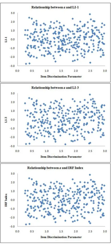
Also, the bivariate distribution ofa-parameter and LIs for all items in the item pool is depicted in Figure 10. It shows that the a-parameter is uniformly distributed and the different LIs are uniformly distributed as well, which is expected as the category parameters are generated originally from a uniform distribution. It is noticeable that there is no positive relationship betweena-parameter and the proposed LIs in the item pool.
Measurement precision. Table 4 presents the overall measurement precision indices. It is expected that the maximum information method will be the most preferable with respect to measurement precision. It is considered as a baseline here for high
precision. Also, it is obvious that the four matching-LI methods using different item indices result in a slight loss in measurement precision compared with the maximum information method. Among these four forms of matching methods, the IRF-index based method is slightly more precise than the other three matching methods; the IRF-index method yields slightly smaller bias, MSE, and largerρθ,θˆ. It is more adequate to claim
Table 4
Overall Measurement Precision Indices Under Different Item Selection Methods (N=1000, M= 300, L=15)
Methods Bias MSE ρθ,θˆ
Matching-LImean 0.004 0.086 .953
Matching-LItrimmed mean 0.008 0.078 .957 Matching-LImedian 0.008 0.078 .957
Matching-LIIRF 0.002 0.076 .958
MI 0.002 0.029 .984
Note. MSE=mean squared error; LI=location index; MI=maximum information. that these four matching methods are comparable in terms of measurement precision.
Conditional Bias and MSE are reported in Table 5. It is clear that the MI method surpasses all the other methods across different ability levels. Also, the overall conditional bias and MSE at different levels are of very low level for all considered item selection methods; conditional bias reaches a maximum of 0.12 in absolute value and conditional MSE reaches a maximum of 0.10. In general, at all levels of θ, the loss in measurement precision for the four LI methods is very small compared to the MI method. The overall measurement precision indices supports the claim that the matching-LI methods are comparable, and this also applied to conditional bias and MSE. All selection methods work slightly better at the three intermediate groups than at the lowest- and highest-20% groups of examinees.