2010/75
■
Low-rank matrix approximation
with weights or missing data is NP-hard
Nicolas Gillis and François Glineur
Center for Operations Research
and Econometrics
Voie du Roman Pays, 34
B-1348 Louvain-la-Neuve
Belgium
http://www.uclouvain.be/core
D I S C U S S I O N P A P E R
CORE DISCUSSION PAPER 2010/75
Low-rank matrix approximation with weights or missing data is NP-hard Nicolas GILLIS 1 and François GLINEUR2
November 2010
Abstract
Weighted low-rank approximation (WLRA), a dimensionality reduction technique for data analysis, has been successfully used in several applications, such as in collaborative filtering to design recommender systems or in computer vision to recover structure from motion.
In this paper, we study the computational complexity of WLRA and prove that it is NP-hard to find an approximate solution, even when a rank-one approximation is sought. Our proofs are based on a reduction from the maximum-edge biclique problem, and apply to strictly positive weights as well as binary weights (the latter corresponding to low-rank matrix approximation with missing data).
Keywords: low-rank matrix approximation, weighted low-rank approximation, missing data, matrix completion with noise, PCA with missing data, computational complexity, maximum-edge biclique problem.
1 Université catholique de Louvain, CORE, B-1348 Louvain-la-Neuve, Belgium. E-mail: [email protected]. 2 Université catholique de Louvain, CORE, B-1348 Louvain-la-Neuve, Belgium. E-mail: [email protected]. This
author is also member of ECORE, the association between CORE and ECARES.
We thank Chia-Tche Chang for his helpful comments. The first author is a research fellow of the Fonds de la Recherche Scientifique (f.R.S.-FNRS).
This paper presents research results of the Belgian Program on Interuniversity Poles of Attraction initiated by the Belgian State, Prime Minister's Office, Science Policy Programming. The scientific responsibility is assumed by the authors.
1
Introduction
Approximating a matrix with one of lower rank is a key problem in data analysis and is widely used for linear dimensionality reduction. Numerous variants exist emphasizing different constraints and objective functions, e.g., principal component analysis (PCA) [15], independent component analysis [5], nonnegative matrix factorization [17], . . . and other refinements are often imposed on these models, e.g., sparsity to improve interpretability or increase compression [6].
In some cases, it might be necessary to attach a weight to each entry of the data matrix corre-sponding to its relative importance [7]. This is for example the case in the following situations:
⋄ The matrix to be approximated is obtained via a sampling procedure and the number of samples and/or the expected variance vary among the entries, e.g., 2-D digital filter design [18], or microarray data analysis [19].
⋄ Some data is missing/unknown, which can be taken into account assigning zero weights to the missing/unknown entries of the data matrix. This is for example the case in collaborative filtering, notably used to design recommender systems [22] (in particular, the Netflix prize com-petition has demonstrated the effectiveness of low-rank matrix factorization techniques [16]), or in computer vision to recover structure from motion [23, 14], see also [3]. This problem is often referred to asPCA with missing data[23, 12], and can be viewed as alow-rank matrix completion problem with noise, i.e., approximate a given noisy data matrix featuring missing entries with a low-rank matrix1.
⋄ A greater emphasis must be placed on the accuracy of the approximation on a localized part of the data, a situation encountered for example in image processing [13, Chapter 6].
Finding a low-rank matrix that is the closest to the input matrix according to these weights is an optimization problem called weighted low-rank approximation (WLRA). Formally, it can be formulated as follows: first, given an m×n nonnegative weight matrix W ∈ Rm+×n, we define the weighted Frobenius norm of anm×n matrix A as ||A||W = (Pi,jWijA2ij)
1
2. Then, given an m×n real matrixM ∈Rm×nand a positive integerr≤min(m, n), we seek anm×nmatrixXwith rank at mostrthat approximatesM as closely as possible, where the quality of the approximation is measured by the weighted Frobenius norm of the error:
p∗= inf
X∈Rm×n||M−X|| 2
W such thatX has rank at mostr.
Since any m×n matrix with rank at most r can be expressed as the product of two matrices of dimensions m×r and r ×n, we will use the following more convenient formulation featuring two unknown matricesU ∈Rm×r and V ∈Rn×r but no explicit rank constraint:
p∗= inf U∈Rm×r,V∈Rn×r ||M−U V T ||2W = X ij Wij(M−U VT)2ij . (WLRA)
Even though (WLRA) is suspected to be NP-hard [14, 24], this has never, to the best of our knowledge, been studied formally. In this paper, we analyze the computational complexity in the rank-one case2 (i.e., forr= 1) and prove the following two results.
Theorem 1. WhenM ∈ {0,1}m×n, andW ∈]0,1]m×n, it is NP-hard to find an approximate solution of rank-one (WLRA) with objective function accuracy less than 2−11(mn)−6.
1
In our settings, the rank of the approximation is fixed a priori. 2
Theorem 2. WhenM ∈[0,1]m×n, andW ∈ {0,1}m×n, it is NP-hard to find an approximate solution of rank-one (WLRA) with objective function accuracy less than 2−12(mn)−7.
It is then NP-hard to find an approximate solution to the following problems: (1) rank-one (WLRA) with positive weights, and (2) rank-one approximation of a matrix with missing data.
The paper is organized as follows. We first review existing results about the complexity of (WLRA) in Section 2. In Section 3.1, we introduce the maximum-edge biclique problem (MBP), which is NP-hard. In Section 3, we prove both Theorems 1 and 2 using a polynomial-time reduction from MBP. We conclude with a discussion and some open questions.
Notation. The set of real matrices with dimension m-by-n is denoted Rm×n; the set Rm×n with component-wise nonnegative entries is denoted Rm+×n; and R0 is the set of nonzero reals. For A ∈
Rm×n, we note A:i theith column ofA, Aj: thejth row ofA, and Aij the entry at position (i, j); for
b∈ Rm×1 =Rm, we note bi the ith entry of b. The transpose of A is AT. The Frobenius norm of a matrixA is defined as||A||2
F = P
i,j(Aij)2, and ||.||2 is the usual Euclidean norm with ||b||22 =
P ib2i. ForW ∈Rm+×n, the weighted Frobenius ‘norm’ of a matrix A is defined3 as||A||2W =
P
i,jWij(Aij)2. The m-by-n matrix of all ones is denoted 1m×n, the m-by-nmatrix of all zeros 0m×n, and In is the identity matrix of dimensionn. The smallest integer larger or equal to x is denoted ⌈x⌉.
2
Previous Results
Weighted low-rank approximation is known to be much more difficult than the corresponding un-weighted problem (i.e., whenW is the matrix of all ones), which is efficiently solved using the singular value decomposition (SVD) [11]. In fact, it has been previously observed that the weighted problem might have several local minima which are not global [24].
Example 1. Let M = 1 0 1 0 1 1 1 1 1 , and W = 1 100 2 100 1 2 1 1 1 .
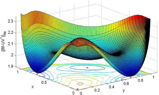
In the case of a rank-one factorization (r = 1) and a nonnegative matrix M, one can impose without loss of generality that U ≥ 0 and V ≥ 0. In fact, one can easily check that any solution U VT is improved by taking its component-wise absolute value |U VT| = |U||V|T. Moreover, we can impose without loss of generality that ||U||2 = 1, so that only two degrees of freedom remain. Indeed, for a given U(x, y) = x y p 1−x2−y2 , with x≥0, y≥0 x2+y2 ≤1 ,
the corresponding optimal V∗(x, y) = argminV ||M −U(x, y)V||2W can be computed easily (it reduces to a weighted least squares problem). Figure 1 displays the surface of the objective function ||M − U(x, y)V∗(x, y)T||W with respect to parametersxandy; we distinguish 4 local minima, close to(√12,0), (0,√1 2), (0,0) and ( 1 √ 2, 1 √
2). We will see later in Section 3 how this example has been generated. However, if the rank of the weight matrix W ∈ Rm+×n is equal to one, i.e., W = stT for some 3
Figure 1: Objective function of (WLRA) with respect to the parameters (x, y).
s∈Rm+ and t∈Rn+, (WLRA) can be reduced to an unweighted low-rank approximation. In fact,
||M −U VT||2W = X i,j sitj(M−U VT)2ij = X i,j sitj(M −U VT)2ij = X i,j p sitjMij −(√siUi:)( p tjVjT:) 2 .
Therefore, if we define a matrix M′ such that M′
ij =√sitjMij ∀i, j, an optimal weighted low-rank approximation (U, V) of M can be recovered from the solution (U′, V′) to the unweighted problem for
matrixM′ usingUi:=Ui′:/√si ∀iandVj:=Vj′:/√tj ∀j.
When the weight matrix W is binary, WLRA amounts to approximating a matrix with missing data. This problem is closely related to low-rank matrix completion (MC), see [2] and references therein, which can be defined as
min
X rank(X) such that Xij =Mij for (i, j)∈Ω⊂ {1,2, . . . , m} × {1,2, . . . , n}, (MC) where Ω is the set of entries for which the values of M are known. (MC) has been shown to be NP-hard [4], and it is clear that an optimal solutionX∗ of (MC) can be obtained by solving a sequence of (WLRA) problems with the same matrixM, with
Wij =
1 if (i, j)∈Ω 0 otherwise ,
and for different values of the target rank ranging fromr = 1 tor= min(m, n). The smallest value of
r for which the objective function ||M −U VT||2W of (WLRA) vanishes provides an optimal solution for (MC). This observation implies that it is NP-hard to solve (WLRA) for each possible value of
r (from 1 to min(m, n)) since it would solve (MC). However, this does not imply that (WLRA) is NP-hard when r is fixed, and in particular when r = 1. In fact, checking whether (MC) admits a rank-one solution can be done easily4.
4
Rank-one (WLRA) can be equivalently reformulated as inf
A ||M−A|| 2
W such that rank(A)≤1,
and, whenW is binary, it is then the problem of finding, if possible, the best rank-one approximation of a matrix with missing entries. To the best of our knowledge, the complexity of this problem has never been studied formally; it will be shown to be NP-hard in the next section.
Another closely related result is the NP-hardness of the structure from motion problem (SFM), in the presence of noise and missing data [20]. Several points of a rigid object are tracked with cameras (we are given the projections of the 3-D points on the 2-D camera planes)5, and the aim is to recover the structure of the object and the positions of the 3-D points. SFM can be written as a rank-four (WLRA) problem with a binary weight matrix6 [14]. However, this result does not imply anything on the complexity analysis of rank-one (WLRA).
An important feature of (WLRA) is exposed by the following example.
Example 2. Let M = 1 ? 0 1
where ? indicates that an entry is missing, i.e., that the weight associated with this entry is 0 (1 otherwise). Observe that ∀(u, v)∈Rm×Rn,
rank(M) = 2 and rank(uvT) = 1 ⇒ ||M −uvT||W >0. However, we have
inf
(u,v)∈Rm×Rn||M−uv T||
W = 0. In fact, one can check that with
u(k)= 1 10−k and v(k)= 1 10k , we have lim k→+∞||M−u (k)v(k)T|| W = 0.
This indicates that when W has zero entries the set of optimal solution of (WLRA) might be empty: there might not exist an optimal solution. In other words, the (bounded) infimum might not be attained. At the other end, the infimum is always attained for W >0 since ||.||W is then a norm.
For this reason, these two cases will be analyzed separately: in Section 3.2, we study the compu-tational complexity of the problem whenW >0, and, in Section 3.3, whenW is binary (the problem with missing data).
3
Complexity of rank-one
(WLRA)
In this section, we use a polynomial-time reduction from the maximum-edge biclique problem to prove Theorems 1 and 2.
5
Missing data arises because the points might not always be visible by the camera, e.g., in case of rotation. 6
3.1 Maximum-Edge Biclique Problem
Abipartite graph is a graph whose vertices can be divided into two disjoint sets such that there is no edge between two vertices in the same set. The maximum-edge biclique problem (MBP) in bipartite graph is the problem of finding a complete bipartite subgraph (abiclique) with the maximum number of edges.
Let M ∈ {0,1}m×n be the biadjacency matrix of a bipartite graph G
b = (V1∪V2, E) with V1 =
{s1, . . . sm},V2 ={t1, . . . tn}and E ⊆(V1×V2) , i.e.,
Mij = 1 ⇐⇒ (si, tj)∈E. The cardinality ofE will be denoted |E|=||M||2F ≤mn.
For example, Figure 2 displays the graph Gb generated by the matrixM of Example 1.
Figure 2: Graph corresponding to the matrix M of Example 1.
With this notation, the maximum-edge biclique problem in a bipartite graph can be formulated as follows [10] min u,v ||M −uv T||2 F uivj ≤Mij, ∀i, j (MBP) u∈ {0,1}m, v ∈ {0,1}n,
whereui= 1 (resp. vj = 1) means that nodesi(resp.tj) belongs to the solution,ui= 0 (resp.vj = 0) otherwise. The constraintuivj ≤Mij, ∀i, j guarantees feasible solutions of (MBP) to be bicliques of
Gb. In fact, it is equivalent to the implication
Mij = 0 ⇒ ui = 0 or vj = 0,
i.e., if there is no edge between vertices si and tj, they cannot simultaneously belong to a solution. The objective function minimizes the number of edges outside the biclique, which is equivalent to maximizing the number of edges inside the biclique. Notice that the minimum of (MBP) is|E| − |E∗|, where|E∗|denotes the number of edges in an optimal biclique.
The decision version of the MBP problem:
GivenK, doesGb contain a biclique with at least K edges?
has been shown to be NP-complete [21] in the usual Turing machine model [8], which is our framework in this paper. Therefore (MBP) is NP-hard.
3.2 Low-Rank Approximation with Positive Weights
In order to prove NP-hardness of rank-one (WLRA) with positive weights (W > 0), let us consider the following instance:
p∗ = min
u∈Rm,v∈Rn||M−uv T
withM ∈ {0,1}m×n the biadjacency of a bipartite graphGb = (V, E) and the weight matrix defined as Wij = 1 if Mij = 1 d ifMij = 0 , 1≤i≤m,1≤j≤n, withd≥1 a parameter.
Intuitively, increasing the value ofdmakes the zero entries of M more important in the objective function, which leads them to be approximated by small values. This observation will be used to show that, fordsufficiently large, the optimal value p∗ of (W-1d) will be close to the minimum |E| − |E∗|
of (MBP) (Lemma 2).
In fact, as the value of parameter d increases, the local minima of (W-1d) get closer to the ‘locally’ optimal solutions of (MBP), which are binary vectors describing the maximal bicliques in
Gb, i.e., bicliques not contained in larger bicliques. Example 1 illustrates the situation: the graph Gb corresponding to matrixM (cf. Figure 2) contains four maximal bicliques{s1, s3, t1, t3},{s2, s3, t2, t3},
{s3, t1, t2, t3}and{s1, s2, s3, t3}, and the weight matrixW that was used is similar to the cased= 100 in problem (W-1d). We now observe that (W-1d) has four local optimal solutions as well (cf. Figure 1) close to (√1 2,0), (0, 1 √ 2), (0,0) and ( 1 √ 2, 1 √
2). There is a one to one correspondence between these solutions and the four maximal bicliques listed above (in this order). For example, for (x, y) = (√1
2,0) we have U(x, y) = (√1 20 1 √ 2)
T, V∗(x, y) is approximately equal to (√2 0√2)T, and this solution corresponds to the maximal biclique{s1, s3, t1, t3}.
Notice that a similar idea was used in [9] to prove NP-hardness of the rank-one nonnegative factor-ization problem minu∈Rm+,v∈Rn+||M−uv
T||
F, where the zero entries ofM were replaced by sufficiently large negative ones.
Let us now prove this formally. It is first observed that for any (u, v) such that||M−uvT||2W ≤ |E|, the absolute value of the row or the column ofuvT corresponding to a zero entry ofM must be smaller than a constant inversely proportional to √4
d.
Lemma 1. Let (i, j) be such that Mij = 0, then ∀(u, v) such that ||M −uvT||2W ≤ |E|,
min max 1≤k≤n|uivk|,1max≤p≤m|upvj| ≤ 4 r 4|E|2 d .
Proof. Without loss of generality uandv can be scaled such that ||u||2 =||v||2 without changing the productuvT. First, observe that since||.||W is a norm,
||uvT||W − p
|E|=||uvT||W − ||M||W ≤ ||M −uvT||W ≤ p
|E|.
Since all entries ofW are larger than 1 (d≥1), we have
||u||2||v||2 =||uvT||F ≤ ||uvT||W ≤ p 4|E|, and then||u||2 =||v||2 ≤ 4 p 4|E|. Moreover d(0−uivj)2 ≤ ||M −uvT||2W ≤ |E|, so that |uivj| ≤ q |E|
d which implies that either
|ui| ≤ 4 q |E| d or |vj| ≤ 4 q |E|
d . Combining above inequalities with the fact that (max1≤k≤n|vk|) and (max1≤p≤m|up|) are bounded above by||u||2 =||v||2 ≤ 4
p
4|E| completes the proof.
Using Lemma 1, we can associate any point (u, v) such that||M −uvT||2
W ≤ |E| with a biclique ofGb, the graph generated by the biadjacency matrix M.
Corollary 1. For any pair(u, v) such that ||M−uvT||2W ≤ |E|, the set
Ω(u, v) =I ×J, with I ={i| ∃j s.t. |uivj|> α} and J ={j | ∃i s.t. |uivj|> α},
where α=q4 4|E|2
d , defines a biclique ofGb.
We can now provide lower and upper bounds on the optimal valuep∗ of (W-1d), and show that it is not too different from the optimal value|E| − |E∗|of (MBP).
Lemma 2. Let 0< ǫ≤1. For any value of parameter dsuch that d≥ 26|ǫE4|6, the optimal value p∗ of (W-1d) satisfies
|E| − |E∗| −ǫ < p∗≤ |E| − |E∗|.
Proof. Let (u, v) be an optimal solution of (W-1d) (there always exists at least one optimal solution, cf. Section 2), and let us note p= |E| − |E∗| ≥ 0. Since any optimal solution of (MBP) plugged in (W-1d) also achieves an objective function equal top, we must have
p∗ =||M−uvT||W2 ≤p=|E| − |E∗|,
which gives the upper bound.
By Corollary 1, the set Ω = Ω(u, v) defines a biclique of (MBP) with |Ω| ≤ |E∗| edges. By construction, the entries in M which are not in Ω are approximated by values smaller than α. If
α=q4 4|E|2
d ≤1, i.e., d≥4|E|2 which is satisfied for 0< ǫ≤1, the error corresponding to a one entry ofM not in the biclique Ω is at least (1−α)2. Since there are at leastp=|E| − |E∗|such entries, we
have
(1−α)2p≤ ||M−uvT||2W. (3.1) Moreover
(1−α)2p >(1−2α)p=p−2αp≥p−2α|E| ≥p−ǫ,
since 2α|E| ≤ǫ ⇐⇒ d≥ 26|ǫE4|6, which gives the lower bound.
This result implies that for ǫ= 1, i.e., for d≥(2|E|)6, we have |E| − |E∗| −1< p∗ ≤ |E| − |E∗|, and therefore computing p∗ exactly would allow to recover |E∗| (since ⌈p∗⌉ = |E| − |E∗|), which is NP-hard. Since the reduction from (MBP) to (W-1d) is polynomial (it uses the same matrixM and a weight matrixW whose description has polynomial length), we conclude that solving (W-1d) exactly is NP-hard. The next result shows that even solving (W-1d) approximately is NP-hard.
Corollary 2. For any d > (2mn)6, M ∈ {0,1}m×n, and W ∈ {1, d}m×n, it is NP-hard to find an approximate solution of rank-one (WLRA) with objective function accuracy less than1−(2mn)3/2
d1/4 . Proof. Let d >(2mn)6, 0< ǫ = (2mn)3/2
d1/4 <1, and (¯u,¯v) be an approximate solution of (W-1d) with objective function accuracy (1−ǫ), i.e.,p∗≤p¯=||M−u¯v¯T||2W ≤p∗+1−ǫ. Sinced= (2mnǫ4)6 ≥
(2|E|)6 ǫ4 , Lemma 2 applies and we have
|E| − |E∗| −ǫ < p∗ ≤ p¯ ≤ p∗+ 1−ǫ ≤ |E| − |E∗|+ 1−ǫ.
We finally observe that ¯p allows to recover |E∗|, which is NP-hard. In fact, adding ǫ to the above
inequalities gives |E| − |E∗|<p¯+ǫ≤ |E| − |E∗|+ 1, and therefore
We are now in position to prove Theorem 1, which deals with the hardness of rank-one (WLRA) with bounded weights.
Proof of Theorem 1. Let us use Corollary 2 withW ∈ {1, d}m×n, and defineW′ = 1
dW ∈ {1d,1}m×n. Clearly, replacing W by W′ in (W-1d) simply amounts to multiplying the objective function by 1d, with ||M −uvT||2W′ = 1
d||M −uvT||2W. Taking d1/4 = 2(2mn)3/2 in Corollary 2, we obtain that for
M ∈ {0,1}m×n andW ∈]0,1]m×n, it is NP-hard to find an approximate solution of rank-one (WLRA) with objective function accuracy less than 1d1−(2mnd1/)43/2
= 21d = 2−11(mn)−6.
Remark 1. Using the same construction as in [10, Theorem 3], this rank-one NP-hardness result can be generalized to any factorization rank, i.e., approximate (WLRA) for any fixed rank r is NP-hard.
Remark 2. The bounds on d have been quite crudely estimated, and can be improved. Our goal was only to show existence of a polynomial-time reduction from (MBP) to rank-one (WLRA).
3.3 Low-Rank Matrix Approximation with Missing Data
Unfortunately, the above NP-hardness proof does not include the case whenW is binary, corresponding to missing data in the matrix to be approximated (or to low-rank matrix completion with noise). This corresponds to the following problem
inf U∈Rm×r,V∈Rn×r ||M −U V T||2 W = X ij Wij(M−U VT)2ij , W ∈ {0,1}m×n. (LRAMD) In the same spirit as before, we consider the following rank-one version of the problem
p∗ = inf
u∈Rm,v∈Rn||M−uv T||2
W, (MD-1d)
with input data matrices M andW defined as follows
M = Mb 0s×Z 0Z×t dIZ and W = 1s×t B1 B2 IZ ,
where Mb ∈ {0,1}s×t is the biadjacency matrix of the bipartite graph Gb = (V, E), d > 1 is a parameter, Z = st− |E| is the number of zero entries in Mb, m = s+Z and n = t+Z are the dimensions ofM and W.
Binary matricesB1∈ {0,1}s×Z and B2 ∈ {0,1}Z×t are constructed as follows: assume the Z zero entries ofMb can be enumerated as{Mb(i1, j1), Mb(i2, j2), . . . , Mb(iZ, jZ)}, and letkij be the (unique) indexk (1 ≤k ≤Z) such that (ik, jk) = (i, j) (therefore kij is only defined for pairs (i, j) such that
Mb(i, j) = 0, and establishes a bijection between these pairs and the set{1,2, . . . , Z}). We now define matricesB1 and as follows: for every index 1≤kij ≤Z, we have
B1(i, kij) = 1, B1(i′, kij) = 0∀i′ 6=iand B2(kij, j) = 1, B2(kij, j′) = 0 ∀j′ 6=j .
Equivalently, each column of B1 (resp. row ofB2) corresponds to a different zero entry Mb(i, j) = 0, and contains only zeros except for a one in positioniwithin the column (resp j within the row).
In the case of Example 1, we get
M = 1 0 1 0 1 1 1 1 1 03×2 02×3 d I2 and W = 13×3 1 0 0 1 0 0 0 1 0 1 0 0 I2 ,
i.e., the matrix to be approximated can be represented as 1 0 1 0 ? 0 1 1 ? 0 1 1 1 ? ? ? 0 ? d ? 0 ? ? ? d .
For any feasible solution (u, v) of (MD-1d), we also note
u= ub ud ∈Rm, ub ∈Rs andud∈RZ, v= vb vd ∈Rn, vb ∈Rt and vd∈RZ.
We will show that this formulation ensures that, asdincreases, the zero entries of the matrixMb (upper left of matrixM, which is the biadjacency matrix ofGb) have to be approximated with smaller values. Hence, as for (W-1d), we will be able to prove that the optimal valuep∗ of (MD-1d) will have to get close to the minimum|E| − |E∗|of (MBP), implying its NP-hardness.
Intuitively, when d is large, the lower right matrix dIZ of M will have to be approximated by a matrix with large diagonal entries since they correspond to one entries in the weight matrixW. Hence
ud(kij)vd(kij) has to be large for all 1≤kij ≤Z. We then have at least eitherud(kij) orvd(kij) large for all kij (recall each kij corresponds to a zero entry inM at position (i, j), cf. definition of B1 and
B2 above). By construction, we also have two entries M(s+kij, j) = 0 and M(i, t+kij) = 0 with nonzero weights corresponding to the nonzero entries B1(i, kij) andB2(kij, j), which then have to be approximated by small values. Ifud(kij) (resp.vd(kij)) is large, then vb(j) (resp. ub(i)) will have to be small since ud(kij)vb(j) ≈0 (resp.ub(i)vd(kij) ≈0). Finally, either ub(i) orvb(j) has to be small, implying thatMb(i, j) is approximated by a small value, because (ub, vb) is bounded independently of the value of d.
We now proceed as in Section 3.2. Let us first give an upper bound for the optimal value p∗ of (MD-1d).
Lemma 3. For d >1, the optimal value p∗ of (MD-1d) is bounded above by|E| − |E∗|, i.e.,
p∗= inf
u∈Rm,v∈Rn||M −uv T||2
W ≤ |E| − |E∗|. (3.2) Proof. Let us build the following feasible solution (u, v) of (MD-1d) where (ub, vb) is an optimal solution of (MBP) and (ud, vd) is defined as
ud(kij) = dK if ub(i) = 0, d1−K if u b(i) = 1, and vd(kij) = dK if vb(j) = 0, d1−K if v b(j) = 1,
withK∈Rand kij the index of the column of B1 and the row ofB2 corresponding to the zero entry (i, j) of Mb (i.e., (i, j) = (ikij, jkij)).
One can check that
(uvT)◦W = ubvb T d1−KB 1 d1−KB2 dIZ ! ,
where◦ is the component-wise (or Hadamard) product between two matrices, so that
p∗ ≤ ||M−uvT||2W =|E| − |E∗|+ 2Z
d2(K−1), ∀K. (3.3)
We now prove a property similar to Lemma 1 for any solution with objective value smaller that
|E|.
Lemma 4. Let d > p|E| and (i, j) be such that Mb(i, j) = 0, then the following holds for any pair (u, v) such that ||M−uvT||2W ≤ |E|: min max 1≤k≤n|uivk|,1≤maxp≤m|upvj| ≤ √ 2|E|34 d−p|E|12. (3.4)
Proof. Without loss of generality we set ||ub||2 = ||vb||2 by scaling u and v without changing uvT. Observing that ||ub||2||vb||2− p |E|=||ubvbT||F − ||Mb||F ≤ ||Mb−ubvTb||F ≤ ||M−uvT||W ≤ p |E|, we have||ub||2||vb||2≤2 p |E|, and ||ub||2=||vb||2 ≤√2|E| 1 4.
Assume Mb(i, j) is zero for some pair (i, j) and let k = kij denote the index of the corresponding column ofB1 and row ofB2 (i.e., such thatB1(i, k) =B2(k, j) = 1). By construction,ud(k)vd(k) has to approximatedin the objective function. This implies (ud(k)vd(k)−d)2 ≤ |E| and then
ud(k)vd(k)≥d− p
|E|>0.
Suppose |ud(k)| is greater than |vd(k)| (the case |vd(k)| greater than |ud(k)|is similar), this implies
|ud(k)| ≥ (d− |E| 1 2)
1
2. Moreover u
d(k)vj has to approximate zero in the objective function, since
B2(k, j) = 1, implying (ud(k)vj−0)2 ≤ |E| ⇒ |ud(k)vj| ≤ p |E|. Hence |vj| ≤ p |E| |ud(k)| ≤ |E|12 d−p |E|12 , (3.5)
and since (max1≤p≤m|up|) is bounded by||ub||2≤√2|E| 1
4, the proof is complete.
One can now associate to any point with objective value smaller than |E| a biclique of Gb, the graph generated by the biadjacency matrixMb.
Corollary 3. Let d >p
|E|, then for any pair (u, v) such that ||M−uvT||2
W ≤ |E|, the set Ω(u, v) =I×J, with I ={i | ∃j s.t. |uivj|> β} and J ={j | ∃is.t. |uivj|> β}, (3.6) where β = √2|E| 3 4 d−√|E| 1 2 , defines a biclique of Gb.
The next lemma gives a lower bound for the value ofp∗.
Lemma 5. Let 0< ǫ≤1. For any value of parameter dthat satisfies d > 8|E|
7 2 ǫ2 +|E| 1 2, the infimum p∗ of (MD-1d)satisfies |E| − |E∗| −ǫ < p∗.
Proof. If|E|=|E∗|, the result is trivial sincep∗= 0. Otherwise, supposep∗≤ |E| − |E∗| −ǫand let
β =
√
2|E|43 d−√|E|
1
2. First observe that d > 8|E|72
ǫ2 +|E| 1
2 is equivalent to 2|E|β < ǫ. Then, by continuity of (MD-1d), for any δ such thatδ < ǫ, there exists a pair (u, v) such that
In particular, let us takeδ= 2|E|β < ǫ. We can now proceed as for Lemma 2. By Corollary 3, Ω(u, v) corresponds to a biclique of Gb, with at most |E∗| edges. Then, for β ≤1, i.e., for d≥2|E|
3 2 +|E| 1 2 satisfied for 0< ǫ≤1, (1−β)2(|E| − |E∗|)≤ ||M−uvT||2W ≤ |E| − |E∗| −δ.
Dividing the above inequalities by |E| − |E∗|>0, we obtain 1−2β <(1−β)2 ≤1− δ
|E| − |E∗|≤1−
δ
|E| ⇒δ <2|E|β,
a contradiction.
Corollary 4. For any d >8(mn)7/2+√mn, M ∈ {0,1, d}m×n, and W ∈ {0,1}m×n, it is NP-hard to find an approximate solution of rank-one (WLRA) with objective function accuracy 1− 2
√
2(mn)7/4 (d−√mn)1/2. Proof. Let d > 8(mn)7/2 +√mn, 0 < ǫ = 2√2(mn)7/4
(d−√mn)1/2 < 1, and (¯u,¯v) be an approximate solution of (W-1d) with absolute error (1−ǫ), i.e., p∗ ≤ p¯= ||M −u¯v¯T||2W ≤ p∗+ 1−ǫ. Lemma 5 applies becaused= 8(mnǫ2)7/2+
√mn
≥ 8(stǫ)27/2 +
√
st≥ 8|Eǫ|27/2 +|E|1/2. Using Lemmas 3 and 5, the rest of the proof is identical as the one of Theorem 1. Since the reduction from (MBP) to (MD-1d) is polynomial (description of matrices W and M has polynomial length, since the increase in matrix dimensions fromMb to M is polynomial), we conclude that finding such an approximate solution for (MD-1d) is NP-hard.
We can now easily derive Theorem 2, which deals with the hardness of rank-one (WLRA) with a bounded matrixM.
Proof of Theorem 2. Replacing M by M′ = 1dM in (MD-1d) gives an equivalent problem with objective function multiplied by d12, since d12||M−uvT||2W =||M′−uv
T
d ||2W. Taking d= 25(mn)7/2+
√
mn in Corollary 4, we find that it is NP-hard to compute an approximate solution of rank-one (WLRA) for M ∈ [0,1]m×n and W ∈ {0,1}m×n, and with objective function accuracy less than
1 d2 1− 2 √ 2(mn)7/4 (d−√mn)1/2 = 21d2 ≥2−12(mn)−7.
4
Concluding Remarks
In this paper, we have studied the complexity of the weighted low-rank approximation problem (WLRA), and proved that finding an approximate solution is NP-hard, already in the rank-one case, both for positive and for binary weights (the latter also corresponding to low-rank matrix completion with noise, or PCA with missing data).
Nevertheless, some questions remain open. In particular,
⋄ When W is the matrix of all ones, WLRA can be solved in polynomial-time. We have shown that, when the ratio between the largest and the smallest entry inW is large enough, the problem is NP-hard (Theorem 1). It would be interesting to investigate the gap between these two facts, i.e., what is the minimum ratio of the entries ofW so that WLRA is NP-hard?
⋄ When rank(W) = 1, WLRA can be solved in polynomial-time (cf. Section 2) while it is NP-hard for general matrix W (with rank up to min(m, n)). But what is the complexity of (WLRA) if the rank of the weight matrixW is fixed and greater than one, e.g., if rank(W) = 2?
⋄ When data is missing, the rank-one matrix approximation problem is NP-hard in general. Nev-ertheless, it has been observed [1] that when the given entries are sufficiently numerous, well distributed in the matrix, and affected by a relatively low level of noise, the original uncorrupted low-rank matrix can be recovered accurately, with a technique based on convex optimization (minimization of the nuclear norm of the approximation, which can be done efficiently). It would then be particularly interesting to analyze the complexity of the problem given additional assumptions on the data matrix, for example on the noise distribution, and deal in particular with situations related to applications.
References
[1] E.J. Cand`es and Y. Plan,Matrix Completion with Noise, in Proceedings of the IEEE, 2009.
[2] E.J. Cand`es and B. Recht, Exact Matrix Completion via Convex Optimization, Foundations of Com-putational Mathematics, 9 (2009), pp. 717–772.
[3] P. Chen, Optimization Algorithms on Subspaces: Revisiting Missing Data Problem in Low-Rank Matrix, International Journal of Computer Vision, 80(1) (2008), pp. 125–142.
[4] A.L. Chistov and D.Yu. Grigoriev,Complexity of quantifier elimination in the theory of algebraically closed fields, Proceedings of the 11th Symposium on Mathematical Foundations of Computer Science, Lecture Notes in Computer Science, Springer, 176 (1984), pp. 17–31.
[5] P. Comon,Independent component analysis, A new concept?, Signal Processing, 36 (1994), pp. 287–314. [6] A. d’Aspremont, L. El Ghaoui, M.I. Jordan, and G.R.G. Lanckriet, A Direct Formulation for
Sparse PCA Using Semidefinite Programming, SIAM Rev., 49(3) (2007), pp. 434–448.
[7] K.R. Gabriel and S. Zamir,Lower Rank Approximation of Matrices by Least Squares With Any Choice of Weights, Technometrics, 21(4) (1979), pp. 489–498.
[8] M.R. Garey and D.S. Johnson, Computers and Intractability: A guide to the theory of
NP-completeness, Freeman, San Francisco, 1979.
[9] N. Gillis and F. Glineur,Nonnegative Factorization and The Maximum Edge Biclique Problem. CORE Discussion paper 2008/64, 2008.
[10] , Using underapproximations for sparse nonnegative matrix factorization, Pattern Recognition, 43(4) (2010), pp. 1676–1687.
[11] G.H. Golub and C.F. Van Loan, Matrix Computation, 3rd Edition, The Johns Hopkins University Press Baltimore, 1996.
[12] B. Grung and R. Manne, Missing values in principal component analysis, Chemom. and Intell. Lab. Syst., 42 (1998), pp. 125–139.
[13] N.-D. Ho, Nonnegative Matrix Factorization - Algorithms and Applications, PhD thesis, Universit´e catholique de Louvain, 2008.
[14] D. Jacobs,Linear fitting with missing data for structure-from-motion, Vision and Image Understanding, 82 (2001), pp. 57–81.
[15] I.T. Jolliffe,Principal Component Analysis, Springer-Verlag, 1986.
[16] Y. Koren, R. Bell, and C. Volinsky, Matrix Factorization Techniques for Recommender Systems, IEEE Computer, 42(8) (2009), pp. 30–37.
[17] D.D. Lee and H.S. Seung,Learning the Parts of Objects by Nonnegative Matrix Factorization, Nature, 401 (1999), pp. 788–791.
[18] W.-S. Lu, S.-C. Pei, and P.-H. Wang, Weighted low-rank approximation of general complex matrices and its application in the design of 2-D digital filters, IEEE Trans. Circuits Syst. I, 44 (1997), pp. 650–655. [19] I. Markovsky and M. Niranjan,Approximate low-rank factorization with structured factors,
[20] D. Nister, F. Kahl, and H. Stewenius, Structure from Motion with Missing Data is NP-Hard, in IEEE 11th Int. Conf. on Computer Vision, 2007.
[21] R. Peeters,The maximum edge biclique problem is NP-complete, Discrete Applied Mathematics, 131(3) (2003), pp. 651–654.
[22] B.M. Sarwar, G. Karypis, J.A. Konstan, and J. Riedl,Item-Based Collaborative Filtering Recom-mendation Algorithms, in 10th International WorldWideWeb Conference, 2001.
[23] H. Shum, K. Ikeuchi, and R. Reddy,Principal component analysis with missing data and its application to polyhedral object modeling, IEEE Trans. Pattern Anal. Mach. Intelligence, 17(9) (1995), pp. 854–867. [24] N. Srebro and T. Jaakkola,Weighted Low-Rank Approximations, in 20th ICML Conference
Recent titles
CORE Discussion Papers
2010/35. Jean-Jacques DETHIER, Pierre PESTIEAU and Rabia ALI. The impact of a minimum pension on old age poverty and its budgetary cost. Evidence from Latin America.
2010/36. Stéphane ZUBER. Justifying social discounting: the rank-discounting utilitarian approach. 2010/37. Marc FLEURBAEY, Thibault GAJDOS and Stéphane ZUBER. Social rationality, separability,
and equity under uncertainty.
2010/38. Helmuth CREMER and Pierre PESTIEAU. Myopia, redistribution and pensions.
2010/39. Giacomo SBRANA and Andrea SILVESTRINI. Aggregation of exponential smoothing processes with an application to portfolio risk evaluation.
2010/40. Jean-François CARPANTIER. Commodities inventory effect.
2010/41. Pierre PESTIEAU and Maria RACIONERO. Tagging with leisure needs.
2010/42. Knud J. MUNK. The optimal commodity tax system as a compromise between two objectives. 2010/43. Marie-Louise LEROUX and Gregory PONTHIERE. Utilitarianism and unequal longevities: A
remedy?
2010/44. Michel DENUIT, Louis EECKHOUDT, Ilia TSETLIN and Robert L. WINKLER. Multivariate concave and convex stochastic dominance.
2010/45. Rüdiger STEPHAN. An extension of disjunctive programming and its impact for compact tree formulations.
2010/46. Jorge MANZI, Ernesto SAN MARTIN and Sébastien VAN BELLEGEM. School system evaluation by value-added analysis under endogeneity.
2010/47. Nicolas GILLIS and François GLINEUR. A multilevel approach for nonnegative matrix factorization.
2010/48. Marie-Louise LEROUX and Pierre PESTIEAU. The political economy of derived pension rights.
2010/49. Jeroen V.K. ROMBOUTS and Lars STENTOFT. Option pricing with asymmetric heteroskedastic normal mixture models.
2010/50. Maik SCHWARZ, Sébastien VAN BELLEGEM and Jean-Pierre FLORENS. Nonparametric frontier estimation from noisy data.
2010/51. Nicolas GILLIS and François GLINEUR. On the geometric interpretation of the nonnegative rank.
2010/52. Yves SMEERS, Giorgia OGGIONI, Elisabetta ALLEVI and Siegfried SCHAIBLE. Generalized Nash Equilibrium and market coupling in the European power system.
2010/53. Giorgia OGGIONI and Yves SMEERS. Market coupling and the organization of counter-trading: separating energy and transmission again?
2010/54. Helmuth CREMER, Firouz GAHVARI and Pierre PESTIEAU. Fertility, human capital accumulation, and the pension system.
2010/55. Jan JOHANNES, Sébastien VAN BELLEGEM and Anne VANHEMS. Iterative regularization in nonparametric instrumental regression.
2010/56. Thierry BRECHET, Pierre-André JOUVET and Gilles ROTILLON. Tradable pollution permits in dynamic general equilibrium: can optimality and acceptability be reconciled?
2010/57. Thomas BAUDIN. The optimal trade-off between quality and quantity with uncertain child survival.
2010/58. Thomas BAUDIN. Family policies: what does the standard endogenous fertility model tell us? 2010/59. Nicolas GILLIS and François GLINEUR. Nonnegative factorization and the maximum edge
biclique problem.
2010/60. Paul BELLEFLAMME and Martin PEITZ. Digital piracy: theory.
2010/61. Axel GAUTIER and Xavier WAUTHY. Competitively neutral universal service obligations. 2010/62. Thierry BRECHET, Julien THENIE, Thibaut ZEIMES and Stéphane ZUBER. The benefits of
cooperation under uncertainty: the case of climate change.
2010/63. Marco DI SUMMA and Laurence A. WOLSEY. Mixing sets linked by bidirected paths. 2010/64. Kaz MIYAGIWA, Huasheng SONG and Hylke VANDENBUSSCHE. Innovation, antidumping
Recent titles
CORE Discussion Papers - continued
2010/65. Thierry BRECHET, Natali HRITONENKO and Yuri YATSENKO. Adaptation and mitigation in long-term climate policies.
2010/66. Marc FLEURBAEY, Marie-Louise LEROUX and Gregory PONTHIERE. Compensating the dead? Yes we can!
2010/67. Philippe CHEVALIER, Jean-Christophe VAN DEN SCHRIECK and Ying WEI. Measuring the variability in supply chains with the peakedness.
2010/68. Mathieu VAN VYVE. Fixed-charge transportation on a path: optimization, LP formulations and separation.
2010/69. Roland Iwan LUTTENS. Lower bounds rule!
2010/70. Fred SCHROYEN and Adekola OYENUGA. Optimal pricing and capacity choice for a public service under risk of interruption.
2010/71. Carlotta BALESTRA, Thierry BRECHET and Stéphane LAMBRECHT. Property rights with biological spillovers: when Hardin meets Meade.
2010/72. Olivier GERGAUD and Victor GINSBURGH. Success: talent, intelligence or beauty?
2010/73. Jean GABSZEWICZ, Victor GINSBURGH, Didier LAUSSEL and Shlomo WEBER. Foreign languages' acquisition: self learning and linguistic schools.
2010/74. Cédric CEULEMANS, Victor GINSBURGH and Patrick LEGROS. Rock and roll bands, (in)complete contracts and creativity.
2010/75. Nicolas GILLIS and François GLINEUR. Low-rank matrix approximation with weights or missing data is NP-hard.
Books
J. GABSZEWICZ (ed.) (2006), La différenciation des produits. Paris, La découverte.
L. BAUWENS, W. POHLMEIER and D. VEREDAS (eds.) (2008), High frequency financial econometrics: recent developments. Heidelberg, Physica-Verlag.
P. VAN HENTENRYCKE and L. WOLSEY (eds.) (2007), Integration of AI and OR techniques in constraint programming for combinatorial optimization problems. Berlin, Springer.
P-P. COMBES, Th. MAYER and J-F. THISSE (eds.) (2008), Economic geography: the integration of regions and nations. Princeton, Princeton University Press.
J. HINDRIKS (ed.) (2008), Au-delà de Copernic: de la confusion au consensus ? Brussels, Academic and Scientific Publishers.
J-M. HURIOT and J-F. THISSE (eds) (2009), Economics of cities. Cambridge, Cambridge University Press. P. BELLEFLAMME and M. PEITZ (eds) (2010), Industrial organization: markets and strategies. Cambridge
University Press.
M. JUNGER, Th. LIEBLING, D. NADDEF, G. NEMHAUSER, W. PULLEYBLANK, G. REINELT, G. RINALDI and L. WOLSEY (eds) (2010), 50 years of integer programming, 1958-2008: from the early years to the state-of-the-art. Berlin Springer.
CORE Lecture Series
C. GOURIÉROUX and A. MONFORT (1995), Simulation Based Econometric Methods. A. RUBINSTEIN (1996), Lectures on Modeling Bounded Rationality.
J. RENEGAR (1999), A Mathematical View of Interior-Point Methods in Convex Optimization.
B.D. BERNHEIM and M.D. WHINSTON (1999), Anticompetitive Exclusion and Foreclosure Through Vertical Agreements.
D. BIENSTOCK (2001), Potential function methods for approximately solving linear programming problems: theory and practice.
R. AMIR (2002), Supermodularity and complementarity in economics. R. WEISMANTEL (2006), Lectures on mixed nonlinear programming.