Air Force Institute of Technology
AFIT Scholar
Theses and Dissertations Student Graduate Works
3-21-2013
Inertial Navigation System Aiding Using Vision
James O. Quarmyne
Follow this and additional works at:https://scholar.afit.edu/etd
Part of theElectrical and Computer Engineering Commons, and theNavigation, Guidance, Control and Dynamics Commons
This Thesis is brought to you for free and open access by the Student Graduate Works at AFIT Scholar. It has been accepted for inclusion in Theses and Dissertations by an authorized administrator of AFIT Scholar. For more information, please [email protected].
Recommended Citation
Quarmyne, James O., "Inertial Navigation System Aiding Using Vision" (2013).Theses and Dissertations. 897. https://scholar.afit.edu/etd/897
INERTIAL NAVIGATION SYSTEM AIDING USING VISION
THESIS
James O. Quarmyne, Second Lieutenant, USAF
AFIT-ENG-13-M-40
DEPARTMENT OF THE AIR FORCE AIR UNIVERSITY
AIR FORCE INSTITUTE OF TECHNOLOGY
Wright-Patterson Air Force Base, Ohio
DISTRIBUTION STATEMENT A.
The views expressed in this thesis are those of the author and do not reflect the official policy or position of the United States Air Force, the Department of Defense, or the United States Government.
This material is declared a work of the U.S. Government and is not subject to copyright protection in the United States
AFIT-ENG-13-M-40
INERTIAL NAVIGATION SYSTEM AIDING USING VISION
THESIS
Presented to the Faculty
Department of Electrical and Computer Engineering Graduate School of Engineering and Management
Air Force Insitute of Technology Air University
Air Education and Training Command in Partial Fulfillment of the Requirements for the Degree of Master of Science in Electrical Engineering
James O. Quarmyne, B.S.E.E. Second Lieutenant, USAF
March 2013
DISTRIBUTION STATEMENT A.
AFIT-ENG-13-M-40
INERTIAL NAVIGATION SYSTEM AIDING USING VISION
James O. Quarmyne, B.S.E.E. Second Lieutenant, USAF
Approved:
Meir Pachter, PhD (Chairman) Date
John F. Raquet, PhD (Committee Member) Date
Abstract
The aiding of an INS using measurements over time of the line of sight of ground features as they come into view of an onboard camera is investigated. The objective is to quantify the reduction in the navigation states’ errors by using bearings-only
measurements over time of terrain features in the aircraft’s field of view. INS aiding is achieved through the use of a Kalman Filter. The design of the Kalman Filter is presented and it is shown that during a long range, wings level cruising flight at constant velocity and altitude, a 90% reduction in the aided INS-calculated navigation state errors compared to a free INS, is possible.
I dedicate this thesis to my loving wife, who supported me every step of the way. I LOVE YOU!
Table of Contents
Page
Abstract . . . iv
Dedication . . . v
List of Figures . . . viii
List of Tables . . . x
List of Symbols . . . xi
List of Abbreviations . . . xiv
1 Introduction . . . 1 1.1 Background . . . 1 1.2 Motivation . . . 2 1.3 Approach . . . 3 2 Literature Review . . . 4 2.1 Introduction . . . 4 2.2 Reference Frames . . . 4
2.2.1 Inertial Reference Frame . . . 4
2.2.2 Earth-Centered, Earth-Fixed Inertial Reference Frame . . . 4
2.2.3 Earth-fixed Reference Frame . . . 5
2.2.4 Navigation Reference Frame . . . 6
2.2.5 The Body Frame . . . 7
2.2.6 Sensor Frame . . . 8
2.3 Coordinate System Transformations . . . 8
2.4 Inertial Navigation . . . 11
2.5 Specific Force and Gravity . . . 11
2.5.1 Specific Force . . . 11
2.5.2 Gravity . . . 12
2.6 INS Equation . . . 13
2.6.1 INS Equations for Common Frames . . . 14
2.6.1.1 Strapdown INS Equation in i-frame . . . 14
2.6.1.2 Strapdown INS Equation in e-frame . . . 14
2.6.1.3 Strapdown INS Equation in n-frame . . . 14
2.7 SLAM . . . 14
2.9 Recent Research . . . 16 3 Methodology . . . 19 3.1 Introduction . . . 19 3.2 Development . . . 19 3.2.1 Aircraft Trajectory . . . 19 3.2.2 INS Alignment . . . 19
3.2.3 Terrain Features Assumptions . . . 19
3.3 Approach and Model Description . . . 20
3.3.1 Dynamics . . . 20
3.3.2 Modeling/Calibrating the Free INS . . . 26
3.3.3 Measurement Equation . . . 28
3.3.4 Synthesis of the Measurement Sent to the KF in Epoch n . . . 38
3.4 Performance of Aided INS . . . 40
3.4.1 Initialization of the KF . . . 42 3.4.2 Kalman Filter . . . 44 3.4.3 Summary . . . 56 4 Simulation Results . . . 58 4.1 Introduction . . . 58 4.2 Simulation . . . 58 5 Conclusion . . . 64
Appendix A: Simulation Results . . . 65
Appendix B: Ground Feature Calculations . . . 73
List of Figures Figure Page 2.1 The I-frame . . . 5 2.2 The i-frame . . . 6 2.3 The e-frame . . . 7 2.4 The n-frame . . . 8
2.5 The b-frame for Airplane . . . 9
2.6 s-frame for INS Sensor and Camera . . . 10
2.7 Relationship Between g, G and Earth’s Rate of a Point Mass . . . 12
2.8 Basic SLAM Problem . . . 15
2.9 Pinhole Camera Geometry . . . 16
3.1 Relationship between the body and inertial frame. . . 21
3.2 Measurement Geometry in General Position. . . 29
3.3 Showing the scenario set up. . . 41
3.4 INS Aiding Using a Kalman Filter . . . 44
4.1 The development of the KF predicted standard deviation and realized position estimates of the unaided INS in the first three measurement epochs. . . 60
4.2 The development of the KF predicted standard deviation and realized position estimates of the aided INS for the first three measurement epochs. . . 61
A.1 The development of the KF predicted standard deviation and realized position estimate of the aided INS during a one hour flight. . . 65
A.2 The development of the KF predicted standard deviation and realized position estimates of the aided INS during a one hour flight for ground features arranged in a straight line. . . 66 A.3 The development of the KF predicted standard deviation and realized position
A.4 The development of velocity estimates in the aided INS during a one hour flight. 68 A.5 The development of attitude estimates in the aided INS during a one hour flight. 69 A.6 The calculated position of the first ground feature. . . 70 A.7 The geolocated second ground feature’s position. . . 70 A.8 A zoomed in view of the development of the KF predicted standard deviation
of the first ground feature’s position in first seven measurement epochs. . . 71 A.9 A zoomed in view of the development of the KF predicted standard deviation
of the second ground object’s position in first seven measurement epochs. . . . 71 A.10 Aircraft and ground objects’ position estimates with KF predicted standard
List of Tables
Table Page
4.1 Standard Deviations and Errors for Simulations . . . 62 B.1 Ground Features on X-Axis: X Position . . . 73 B.2 Ground Features on X-Axis: Y Position . . . 73 B.3 Y Positions of Laterally Staggered Ground Features on Both Sides of X-Axis . 73
List of Symbols Symbol Page Cab DCM fromb toa Frame . . . 10 h Altitude . . . 19 v Velocity . . . 19 x xDirection . . . 19 y yDirection . . . 19 z zDirection . . . 19
yp Inertial FrameyPosition of Ground Feature . . . 20
ψ Aircraft Yaw Angle . . . 20
θ Aircraft Pitch Angle . . . 20
φ Aircraft Roll Angle . . . 20
δx Navigation Error State Vector . . . 21
δP Position Error Vector . . . 21
δV Velocity Error Vector . . . 21
δΨ Angle Error Vector . . . 21
δu Disturbance Vector . . . 21
b Indicates Body Frame . . . 21
(n) Indicates Navigation Frame . . . 23
→ f Specific Force Measured by Accelerometer . . . 23
→ a Total Aircraft Acceleration . . . 23
→ g Specific Gravity Vector . . . 23
fx(n) Specific Force Measured by Longitudinal Accelerometer . . . 23
fy(n) Specific Force Measured by Lateral Accelerometer . . . 23
fz(n) Specific Force Measured by Vertical Accelerometer . . . 23
a Longitudinal Acceleration of Aircraft . . . 23
t Current Time . . . 24
T Duration of a Measurement Epoch . . . 24
Aa Continuos-Time Dynamics Matrix . . . 25
∆T Sampling Interval . . . 25
l Discrete Time Step Counter . . . 25
L Number of Bearing Measurements in an Epoch . . . 25
Aad Discrete-Time Dynamics Matrix . . . 25
xp Inertial Frame xPosition of Ground Feature . . . 25
m Number of Unknown Tracked Features . . . 25
σa Standard Deviation of the Uncertainty of the Accelerometer Bias . . . 26
σg Standard Deviation of the Uncertainty of the Gyroscope Bias . . . 26
N Number of Measurement Epochs . . . 27
α Accelerometer Bias Constant . . . 27
β Gyroscope Bias Constant . . . 27
xf xCoordinate of Ground Feature on Camera Focal Plane . . . 28
yf yCoordinate of Ground Feature on Camera Focal Plane . . . 28
f Focal Length . . . 28
zp Ground Feature Elevation . . . 30
c Indicates Calculated Value from INS . . . 31
m Indicates a Measured Value . . . 31
H(l) Time Dependent Measurement Matrix . . . 33
u Indicates Ground Feature’s Position is Unknown . . . 33
k Indicates Ground Feature’s Position is Known . . . 34
z Measurements . . . 36
x True Navigation State . . . 37
δxF Navigation State Error of Free INS . . . 37
(n) Current Measurement Epoch . . . 38
P Covariance Matrix . . . 42
ˆ δx Kalman Filter Estimates . . . 44
K Kalman Gain . . . 45
List of Abbreviations
Abbreviation Page
GPS Global Positioning System . . . 1
INS Inertial Navigation Systems . . . 1
LO Low Observable . . . 2
HVT High Value Target . . . 2
SLAM Simultaneous Localization and Mapping . . . 3
CG center of gravity . . . 7
DCM Direction Cosine Matrix . . . 10
KF Kalman Filter . . . 15
SS State Space . . . 15
LOS Line Of Sight . . . 17
UAVs Unmanned Aerial Vehicles . . . 20
RHS Right Hand Side . . . 32
LHS Left Hand Side . . . 32
Inertial Navigation System Aiding Using Vision
1 Introduction
1.1 Background
Navigation can be defined as the process of reading, and controlling the movement of a craft or vehicle from one place to another[1]. Navigation is achieved by comparing the navigator’s position to known locations and this can be done in many different ways. These include but are not limited to an individual using a map, a vehicle using Global Positioning System (GPS), or an aircraft using an Inertial Navigation Systems (INS) in combination with a GPS to provide very precise navigation.
An aircraft using an Inertial Navigation Systems (INS) aided by GPS measurements is afforded very precise navigation. GPS is very accurate but may be occasionally denied due to outages. It is therefore prudent to have workarounds for situations where the precision available from GPS is denied. Aiding INS using the measurements of terrain features’ bearings render the integrated navigation system less dependent on GPS. This is desirable since the vision-aided INS will be an autonomous navigation system which is self-contained and not susceptible to jamming and spoofing. The crucial issues of detection of ground features in a camera’s field of view and the autonomous tracking of these features/image registration, [5], [7], and [6] are not addressed in this paper. The focus is on gaining an understanding of the INS aiding action afforded by bearings measurements over time of possibly unknown ground features.
In [12] it was shown using covariance analysis that the rate of growth of position uncertainty is significantly reduced when the aircraft uses terrain features bearing
measurements to aid the INS. The same applies to the uncertainty in velocity and the aircraft’s Euler angles.
This paper focuses on the mechanization of the Kalman Filter (KF) for vision aided INS. It is shown that using the measurement over time of the bearings of ground features in an aircraft’s field of view, a KF can significantly reduce the errors in the aircraft’s navigation states in a GPS denied environment. A cross country navigation scenario using the concept of “bootstrapping” where new ground features as they come in the camera’s field of view are sequentially geolocated and then tracked during their residence in the camera’s field of view, is analyzed. The Kalman Filter is mechanized in the context of Simultaneous Localization and Mapping (SLAM).
It is shown that the synergetic action of the designed Kalman Filter and the
geolocation algorithm makes SLAM possible and using the “bootstrapping” concept long range flight which entails INS aiding using bearing measurements of unknown ground features is feasible-this, provided that the image registration problem is solved.
1.2 Motivation
Consider a Low Observable (LO) aircraft carrying a LO munition on a mission into a territory to eliminate a High Value Target (HVT). The objective is to eliminate the target with as minimal collateral damage as possible, so precision is of utmost importance. The HVT is limited to a small area such that it takes approximately an hour to fly from the origin of the military base. The adversary actively uses anti-GPS technologies, thus denying the precision and accuracy of GPS. The aircraft has a navigation quality INS but the duration of the flight is long enough that the errors produced by the INS are too large for precise lock onto the HVT. The pilot needs a better navigation solution, but does not want to inform the enemy of the aircraft’s presence by using active navigation techniques, such as radar. The autonomy of the INS is good for stealth but is not enough to provide precise navigation solution given the errors that accumulate over time.
The proposed solution is to use the bearing measurements of known and unknown ground features to aid the navigation provided by the INS. The aircraft uses its camera to geolocate ground features, track those features to aid the INS, and using that aided estimate geolocate new features as the original features leave the camera’s FOV. This aiding scheme constrains the error enough to obtain target solution. The on board
munition, with its lower quality INS, uses a similar visual scheme. It looks within the area given during the mission briefing for the HVT. The munition impacts the HVT and the aircraft leaves the scene without emitting any signal that will give away its location.
1.3 Approach
This paper will be structured such that each chapter will begin with a brief description of topics that will be forthcoming. Chapter 2 provides information on the various coordinate frames of reference that is used when working with an INS, the transformations between the coordinate frames, INS mechaniztion equations, a brief discussion of Simultaneous Localization and Mapping (SLAM) and concludes with recent research in the field. Chapter 3 shows the mathematical development of the 2-D case, including the dynamics and measurement model development, the state space
representation and the use of the KF mechanization. This information is then extended to look at the 3-D case for both a horizontal flight and a vertical fall. Chapter 4 looks at the results of the covariance analysis. Finally, Chapter 5 summarizes the key points of the paper, focusing on the impact the INS aiding scheme provided.
2 Literature Review
2.1 Introduction
This section provides information on the various coordinate frames of reference that is used when working with INS. Section 2.2 discusses the different coordinate frames of reference. Section 2.3 discuses the transformations between the various coordinate frames. Section 2.4 discusses the fundamentals of inertial navigation, including a brief discussion of the sensors used and how they work. Section 2.6 discusses the fundamental INS equation and the INS equations for some common frames. Section 2.7 discusses SLAM. Section 2.8 discusses the camera model that will be used as a sensor. Finally, Section 2.9 reviews recent research that contributed to this paper.
2.2 Reference Frames
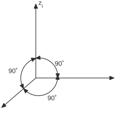
2.2.1 Inertial Reference Frame. The Inertial Reference Frame which is also
known as the “true” inertial frame is denoted as the I-frame. The I-frame is located in the sky and it is in this frame that Newton’s laws apply. All reference frames used in this paper follow the right handed reference system. The I-frame is shown in Figure 2.1.
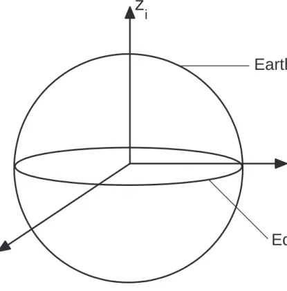
2.2.2 Earth-Centered, Earth-Fixed Inertial Reference Frame. The Earth-centered,
Earth-Fixed (ECEF) inertial reference frame, as the name imply, has its origin fixed to the center of the earth. It is denoted as the i-frame and moves with the earth relative to the I-frame. With the Earth modelled as an ellipsoid, the axes of the i-frame are partially fixed to the I-frame and are defined as follows:
• xi-axis,along the Equator and pointing towards the first star in the Aries
• zi-axis,points towards the North Pole
90˚
90˚
90˚
z
ix
iy
iFigure 2.1: The I-frame
The i-frame in the earth model is shown in Figure 2.2.
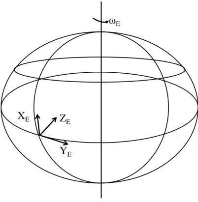
2.2.3 Earth-fixed Reference Frame. The Earth-fixed reference frame has its origin
fixed to an arbitrary point on the surface of the Earth. The axes of the e-frame are defined as follows:
• xe-axis points to the North
• ye-axis points to the east
• ze-points to the gravitational center of the Earth.
The e-frame is shown in Figure 2.3. Since the e-frame is fixed to an arbitrary point on the
surface of the earth, it moves at the earth rate. The rotation between the i-frame and the e-frame is denoted byθe ie, whereθ e ieis given by: θe ie =ωe(t−t0)
z
i
x
i
y
i
Equator
Earth
Figure 2.2: The i-frame
andωeis the sidereal rate of the earth≈360◦/day
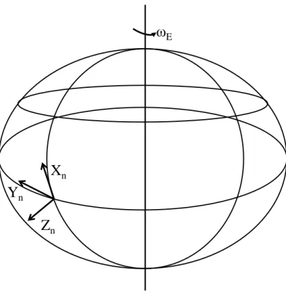
2.2.4 Navigation Reference Frame. The navigation frame, also known as the local
level frame is denoted as the n-frame. The origin of this reference frame is located on a plane which is tangential to the surface of the Earth, wherez=0 is for the surface of the Earth. The e-frame is fixed to the earth, but the n-frame is not. The axes of the n-frame are defined as follows:
• xn-axis,points from the origin to the North pole
• yn-axis,points to the west
• zn-axis,points down away from the center of the Earth
X
EY
EZ
Eω
EFigure 2.3: The e-frame
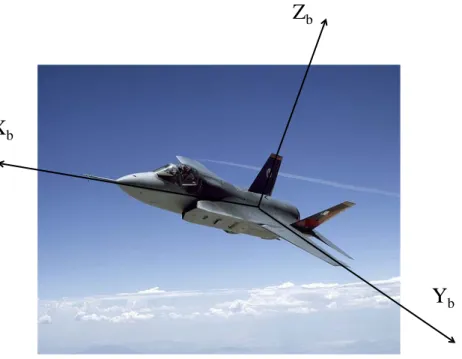
2.2.5 The Body Frame. The body frame, denoted as the b-frame is rigidly attached
to the body of a vehicle (airplane, car, ship, etc.). The origin is located somewhere on the body, either the center of gravity (CG) or something measurable. The axes do not change with changes to an aircraft’s trajectory or orientation of a car. Due to the fact that an aircraft loses fuel in the cause of flight and the center of gravity will consequently change, the origin of the body frame will be fixed to the origin of the camera in this paper. The body axes are defined as follows:
• xb-axis,points out of the nose of the aircraft
• yb-axis,points out of the left wing of the aircraft
• zb-axis,points out of the top of the aircraft
X
nY
nZ
nω
EFigure 2.4: The n-frame
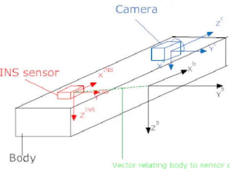
2.2.6 Sensor Frame. The sensor frame, denoted as the s-frame is defined by the
designer using the right handed reference system. It is completely up to the designer to define the origin and axes of the s-frame. Figure 2.6 shows two sensors (INS and camera) with their respective s-frames in relation to the b-frame of an object whose origin is at the CG. Again, for reasons discussed in sub-section 2.2.5 the origin of the body frame will be co-located with the origin of the camera frame in this paper.
2.3 Coordinate System Transformations
In INS computations, it is often convenient to convert the different frames to a single frame (often the navigation frame) for easy calculations. In order to transform points and vectors from one frame to the other, there is the need to perform either translation, rotation, or both. Translation is ann×1 vector that relates the origins of two frames of
X
bY
bZ
bFigure 2.5: The b-frame for Airplane
interest. The translation of a pointP, from a-frame to b-frame in the a-frame is denoted by Pa
ab. Rotations on the other hand are defined with respect to the orthogonal right-handed axis set. Rotation of a set of axes in one frame to another frame can be done in one of three ways, namely:
1. Euler angles(φ, θ, ψ): This is a transformation of one frame to another by three successive rotations about three different axes taken in turn [13]. It is worth noting that the order of rotation matters; rotation in the order (φ, θ, ψ) is different from rotation in the order (θ, ψ, φ).
2. Quaternions (4×1 vector): The quaternion attitude representation allows a transformation from one coordinate frame to another to be effected by a single rotation about a vector defined in the reference frame. The quaternion is a
Figure 2.6: s-frame for INS Sensor and Camera
four-element vector representation, the elements of which are functions of the orientation of this vector and the magnitude of the rotation.
3. Direction Cosine Matrix (DCM) (3×3 matrix): The Direction Cosine Matrix (DCM), is a 3×3 matrix, the columns of which represent unit vectors in body axes projected along the reference axes. The DCM from a b-frame to an a-frame is denoted by Ca
b, which is written as follows:
Cab = C11 C12 C13 C21 C22 C23 C31 C32 C33 (2.1)
Where the element in theith row and thejth column represents the cosine of the angle between thei-axis of the a-frame and thej-axis of the b-frame.
This paper uses DCM for coordinate system transformations. For right-handed, orthonormal reference frames, some DCM rules are as follows:
Det Cba= C a b = 1 (Cba) −1 =( Cab) T = Cab Cac =C a bC b c 2.4 Inertial Navigation
This section provides an overview of the basic principles of inertial systems. To navigate, knowledge of the measurements of specific force and angular rates are required. These measurements are provided by an INS, which consists of accelerometers and gyros. Accelerometers measure specific force, while gyros measure angular rate. An INS is a self-contained and nonjammable navigation instrument that provides redundancy for radio navigation systems that can experience interference or be jammed; however, an INS does suffer from drift, the unbounded growth of errors over time. Even, with perfect alignment, accelerometer biases and gyro drift causes the errors in INS to grow over time [10].
2.5 Specific Force and Gravity
2.5.1 Specific Force. From Newton’s Second Law of Motion, the force,FIacting
on a body of massm, moving with an acceleration of ¨pI in the inertial frame is given by:
FI =mp¨I (2.2)
Accelerometers, as was mentioned earlier, measure specific force,fI, and it is defined as the inertial force,FI, per unit massm,required to produce the acceleration ¨pI. This relationship is given by Equation 2.3.
fI , FI
m ≈ fi (2.3)
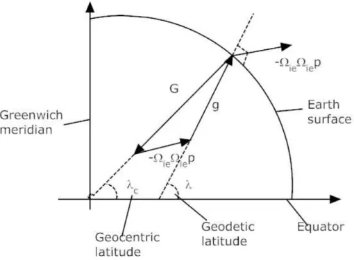
Figure 2.7: Relationship Between g, G and Earth’s Rate of a Point Mass
2.5.2 Gravity. The acceleration ¨pI,acting on a particle in a gravitational field is given by the fundamental equation of inertial navigation as:
¨
pI = fi+Gi (2.4)
Gravityg, is then defined by equation 2.5 below.
g=G(p)−ΩieΩiep (2.5)
where G is the Earth’s gravitational force acting on the particle at positionpandΩieis the centrifugal force pulling outward due to the rotation of the earth. It is worth noting that gravity is not an inertial force. This relationship is as depicted in Figure 2.7.
This effect is not very significant, since the centrifugal force is only a fraction of the gravitational force:
kΩieΩiepk ≈
1
2.6 INS Equation
Consider relating the time derivative of vectors in rotating reference frames. From vector addition: raa 0p =r a a0b0 +r a b0p (2.7) wherera a0p andr a
a0b0 and it is the desire to findr a b0p in theb-frame: rbb 0p = C b ar a b0p =C b a(r a a0p−r a a0b0)= C b ar a a0p+r b b0a0 (2.8)
For short-hand, write as
pb= Cbapa+rbba (2.9)
Taking the time derivative ofpbyields:
d dt p b ! ,vb= d dt C b a ! pa+Cba d dt p a ! + d dt r b ba ! (2.10) = CbaΩaabpa+Cba d dt p a ! + d dt r b ba ! (2.11) vb= d dt r b ba ! +Cba(Ω a abp a+ va) (2.12)
where dtd(rbba) accounts for the relative velocity betwwen thea-frame andb-frame, CbaΩ
a abp
a
is the instantaneous velocity of prelative to theb-frame due to the relative rotation of thea-frame, andCb
av
ais the instantaneous velocity of
pin thea-frame transformed intob-frame. Taking another time derivative of Eq. 2.12 results in:
d dt v b ! ,ab = d 2 dt2r b ba+ d dt " Cba (Ωaabpa+va) # (2.13) =r¨bba+ dC b a dt (Ω a abp a+ va)+Cbad(Ω a abp a+ va) dt (2.14) =r¨bba+ CbaΩaab (Ωaabpa+va)+Cba(Ω˙aabpa+Ωaabva)+Cbaaa (2.15) ab =r¨bba+Cba[(Ω a abΩ a ab+Ω˙ a ab)p a+ 2Ωaabva+aa] (2.16) Eq. 2.16 represents the fundamental relationship for an INS.
2.6.1 INS Equations for Common Frames. The previous section dealt with INS equations for some arbitrary frames. This section will briefly provide the strapdown INS equations for the following frames:
2.6.1.1 Strapdown INS Equation in i-frame. In the i-frame, Eq. 2.16 reduces
to
d2pi
dt2 =C
i
bfb+gi (2.17)
2.6.1.2 Strapdown INS Equation in e-frame. In the e-frame, Eq. 2.16 reduces
to d2pe dt2 =C e bfb+ge−2Ω e ieve (2.18)
2.6.1.3 Strapdown INS Equation in n-frame. In the n-frame, Eq. 2.16 reduces
to d2p n dt2 =C n bfb+gn−(2Ωienvn+ Ωnen)vn (2.19) 2.7 SLAM
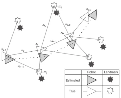
Maps are needed to depict an environment for planning and navigation. They may or may not be readily available depending on the environment of interest. In the case that they are not readily available (due to topographical changes or an unfamiliar indoor environment), the techniques of SLAM come in very handy. SLAM is a process by which a mobile robot or an autonomous vehicle can build a map of an environment and at the same time use this map to deduce its location [2]. The essential SLAM problem is shown in Figure 2.8 [2]
To understand SLAM, consider a mobile robot having an onboard sensor, a camera for example, moving through an unknown environment with noa prioriinformation about the environment. The robot probabilistically estimates its own position and uses the onboard camera to estimate the position of unknown landmarks. It is a recursive process
Figure 2.8: Basic SLAM Problem. The essential problem of SLAM requires the simultaneous estimation of both robot or autonomous vehicle and landmark positions. Neither position is truly known[2].
where the robot uses its position to estimate the position of unknown ground features and then uses the the estimates of the ground features to estimate its own position. This recursive process is typically achieved through the use of a Kalman Filter (KF).
With the introduction of each additional unknown ground feature, the states used in the State Space (SS) equation of the KF increases depending on the type information required by the KF for its estimation. In this paper, thexandypositions of stationary ground features are the informtation of interest so with the addition of an unknown ground feature whose position is to be estimated, the states in the SS of the KF increase by two. This is because stationary ground features are at zero elevation, so only the xandy positions of the ground features are considered. Likewise, with the drop of ground feature by the sensor (camera) because it is no longer in its FOV the states in the SS of the KF decrease by two.
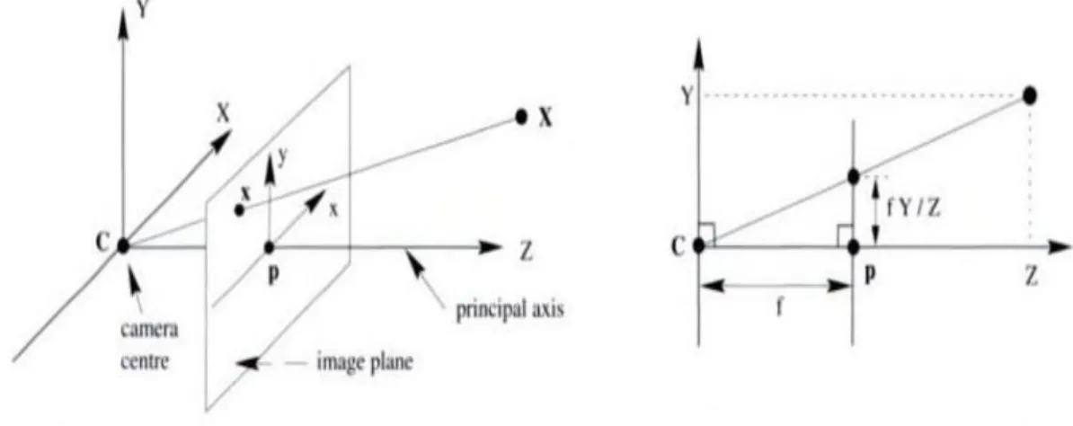
2.8 Camera Model
In this paper, the camera will be modelled as the basic pinhole camera where it is assumed that there are no camera distortions. Camera caliberation will therefore not be considered. The basic pinhole camera is shown in Figure 2.9. The focal length of the
Figure 2.9: Pinhole Camera Geometry. C is the camera centerand p the principal point. The camera center is placed at the coordinate origin [4].
camera is f. Features are considered as points which are projected in space onto an image plane. A point in space with coordinatesX=(X,Y,Z)T is projected onto the image plane. From the geometry, it can be computed by similar triangles that (X,Y,Z)T maps onto the point (fX/Z,fY/Z,f)T on the image plane[4]. Ignoring the final image coordinate, it can be seen that
(X,Y,Z)T 7→(fX/Z,fY/Z)T (2.20)
2.9 Recent Research
In [10], Pachter et. al researched the idea of using bearings-only measurements for aiding INS. This was a theoretical work, where no simulations or empirical data were used to substantiate the theory. The significance of this research was the development of the
mathematics for observing the Line Of Sight (LOS) angle measurements to a ground feature over time and using that information to update an INS. The update was theorized to constraining the unbounded errors developed by an INS if it were allowed to operate freely.
In [3], Giebner aided an aircraft INS using visual measurements when the aircraft flies in a circular orbit around a several ground features. A KF was used to achieve the aiding and this was done both in simulation and in an actual test environment. It was found that the uncertainty in the aircraft’s position after six minutes of flight time, was reduced from 350 meters, in the unaided INS case, down to 50 meters, in the aided INS case, when the visual measurements were combined with barometric altimeter readings.
In [9], Pachter and Mutlu explored the observability of a vision-aided INS. The bearing measurements used were time dependent because the position of the ground feature(s) being tracked by the aircraft changed with time. The time dependent
measurement matrix prompted the use of observability Grammian. It was determined that using the bearings-only visual measurements of a single ground feature to aid the INS, the observability Grammian was rank deficient, making the INS aiding action incomplete. In order for full rank observability Grammian and thereby have complete INS aiding action, a second ground feature had to be simultaneously tracked. Complete INS aiding action means all of the navigation states receive some improvement from the measurement when compared to the unaided INS.
In [2], Durrant-Whyte and Bailey provided the origins of SLAM. It was shown how various filter methods can be used to implement SLAM using the limited information in a robot’s environment. The uncertainty of detected features, as well as the navigation estimate, was shown to be dependent on the number of measurements taken. The more measurements that were taken, the less the uncertainty. In a scenario where a robot was remotely piloted through an indoor environment, a pilot with no visual access of the robot,
the robot autonomously returned to its starting point using map that it build up during the navigation process.
In [14], Veth looked at the fusion of imaging and inertial sensors for navigation. A statistical feature projection technique was developed which utilizes inertial
measurements to predict vectors in the feature space between images. The feature matches and inertial measurements were used to estimate the navigation trajectory on-line using an extended Kalman filter.
This paper is a continuation of [12]. In [12] it was shown using covariance analysis that the rate of growth of position uncertainty is significantly reduced when the aircraft uses terrain features bearing measurements to aid the INS. The same applies to the uncertainty in velocity and the aircraft’s Euler angles. The method used for geolocating new ground features were crude, where only the aircraft position was used in the geolocation process. This paper will look at a more accurate method (include the other navigation states in the geolocation of ground features) of calculating the covariances and implement a KF in a simulation analysis to substantiate the theory.
3 Methodology
3.1 Introduction
This chapter is broken up into three main sections. Section 3.2 discusses the navigation scenario that is considered for the dynamics model development. Section 3.3 discusses the approach that is taking in calibrating the unaided INS with small angle assumptions, measurement model development, the measurement equations that are sent to the KF, and how the calculations are accomplished. Section 3.4 discusses the
performance of the aided INS, which includes the KF and its initialization at the beginning of each epoch.
3.2 Development
The navigation scenario is as follows:
3.2.1 Aircraft Trajectory. The aircraft is flying wings-level at a constant altitudeh.
The ground speed of the aircraft is constant and the aircraft flies in the positivexn direction.
3.2.2 INS Alignment. The initial INS alignment is considered to be “perfect”.
That is, at the start of the flight at altitudehand velocityvin the positivexndirection, the exact aircraft’s position, velocity, and attitude are known with very small errors. The emphasis is on the contribution of the inertial instruments’ errors to the INS navigation state errors. In this respect it is assumed that thex,y, andzaccelerometers are of the same quality; also thex,y, andzgyroscopes are of the same quality and the instruments’
measurement error is modeled as a random bias.
3.2.3 Terrain Features Assumptions. At all time two ground features need to be
features to come into the aircraft camera’s field of view are known. The position of
subsequent features are not known but these are geolocated as they come into the camera’s field of view `a la SLAM. Bearing measurements to these newly acquired features are subsequently taken, hence the “bootstrapping” concept. Obviously, for vision-aided navigation to be possible, one cannot fly over featureless terrain and the features need to be more or less regularly spaced. Hence, without loss of generality it is assumed that the features are nominally equally spaced in the positive xndirection and are at zero, a.k.a. known, elevation. Two scenarios are considered. First the ground features are arranged in a perfect straight line along the aircraft’s trajectory, and second, the ground features are laterally staggeredyp meters about thexn axis. Thus, in the first navigation scenario,ypis zero meters and all the terrain features are on thexn axis. The Earth is assumed flat and nonrotating. This assumption is reasonable considering the relatively short range and/or the tactical grade specification of the gyros and accelerometers of small Unmanned Aerial Vehicles (UAVs) for which this autonomous navigation system is being developed.
Kalman filtering in a SLAM scenario where the aircraft uses inertial navigation is considered. Our novel approach to SLAM is rooted in the theory of inertial navigation, as opposed to robotics or computer science.
3.3 Approach and Model Description
3.3.1 Dynamics. The navigation n-frame is the Earth fixed “inertial” (xn,yn,zn) frame. The aircraft’s body axes are (xb,yb,zb). The aircraft’s and camera’s position in the navigation frame is (x,y,z), withψ,θ, andφas its Euler angles. A strapdown [13] INS arrangement is considered. When flying over a non-rotating and flat Earth as shown in Figure 3.1, the INS error dynamics can be considerably simplified [11], [12], [13]. The simplified dynamics of the INS errors in state space notation, also known as the error
equations, areδ˙x= Aδx+Γδu, where the navigation error state vectorδxgiven by
δx=[ δP δV δΨ ]T (3.1)
are the errors in the navigation state’s positionδP, velocityδV, and anglesδΨ, and the disturbancesδuare the three accelerometers’ and the three rate gyroscopes’ random biases
δu=[ δfb
x δfyb δfzb δωbx δωby δωbz ] T
(3.2)
The superscriptbindicates that the body frame of reference is being used. The errors in
Figure 3.1: Level Flight at Constant Altitude Along the xn-axis
the angles,δΨ, are given by
δΨ=−δCnbCbn (3.3)
and
whereCbnis the DCM andδΨis the skew symmetric matrix formed from the angle errors vectorδΨaccording to Eq. (3.4).
For small Euler anglesψ, θ, φ,the DCM
Cnb(ψ, θ, φ)= 1 −ψ θ ψ 1 −φ −θ φ 1 (3.5)
and therefore its perturbation
δCnb= 0 −δψ δθ δψ 0 −δφ −δθ δφ 0 (3.6)
For constant altitude flight in the direction of thexnaxis, the nominalCbn= I3. Thus, using Eq. (3.3) the following is calculated
δΨ= 0 δψ −δθ −δψ 0 δφ δθ −δφ 0 (3.7)
and sinceδΨ=δΨ×the errors in the aircraft’s Euler angles are recovered
δΨ =[ −δφ −δθ −δψ ]T (3.8)
Hence, the navigation state’s error vector is
δx= [ δx δy δz δvx δvy δvz −δφ −δθ −δψ ]T (3.9) and the INS error state equations are
δ˙x= 03×3 I3×3 03×3 03×3 03×3 F( n) 3×3 03×3 03×3 03×3 δx+ 03×3 03×3 Cb n 03×3 03×3 −Cb δu (3.10)
whereF(n) =f(n)×is the skew symmetric matrix form of the specific force vectorf(n). The superscript(n)indicates that the inertial navigation frame of reference is being used. The specific force measured by the accelerometer
→
f, total aircraft acceleration→a, and the specific gravity vector→gare related according to Eq. 2.4 by→f = →a−→g, that is, f(n)= a(n)−g(n). During wings level flight
a(n) = a 0 0 , g(n) = 0 0 −g
Therefore the nominal specific force components during constant altitude, wings level flight are fx(n)=a, fy(n)=0 and fz(n)= g, wheregis the acceleration of gravity andais the longitudinal acceleration of the aircraft. Thus,
f(n) = fx(n) fy(n) fz(n) = a 0 g (3.11)
Eqs. (3.10) and (3.11) represent the dynamics of the navigation state’s error, (δP, δV, δΨ), under the assumption that the Earth is flat and non-rotating. The meaning of the angular errors’ vectorδΨ, that is, its relationship to the Euler angles’ errors, is determined by the aircraft’s trajectory, that is, the nominal DCMCnb. In the special case of wings level flight when the body and navigation frames are aligned as shown in Figure 3.1, the angular errors are the Euler angles. However, having negative angle error states is unorthodox. In order for the navigation state error to be
δx= [ δx δy δz δvx δvy δvz δφ δθ δψ ]T (3.12)
the dynamics Eq. (3.10) is modified as follows
δ˙x= 03×3 I3×3 03×3 03×3 03×3 −F( n) 3×3 03×3 03×3 03×3 δx+ 03×3 03×3 Cb n 03×3 03×3 Cbn δu (3.13)
and for “perfect” INS alignment with very small uncertainties, δx(0)= δP(0) δV(0) δΨ(0) 9×1 where (δP(xb)(0), δP(yb)(0), δPz(b)(0) ∼ N(03×1,1×10−6I3) (δV(xb)(0), δV(yb)(0), δVz(b)(0)∼ N(03×1,1×10−16I3) (δΨ(φb)(0), δΨ(θb)(0), δΨ(ψb)(0)∼ N(03×1,1×10 −8 I3)
Since this is wings level, constant altitude flight, in the direction of the xnaxis, the nominal, true navigation variables are
x= x0+vxt+ 12at2,y= 0,z= h,φ=θ=ψ =0. These variables are non-dimensionalized as follows x→ x h, y→ y h, z→ z h, vx → vx v , vx → vx v, vz → vz v, δfx → δfx g , δfy → δfy g , δfz → δfz g , δωb x →h δωb x v , δω b y →h δωb y v , δω b z →h δωb z v , t→tv h, T →T v h,
wheretis the current time, andT is the length of a measurement epoch. The non-dimensional parameters are
g, hg
v2 and a,
ha v2 During cruise,a≡0. If, for example,
h=1000[m], v=100 m sec , g= 10 m sec2 ,
the non-dimensional parameterg=1. Since the ground features are spaced 1 [km] apart, the duration of a nondimensional measurement epochT =1.
It is assumed that the sensor errors are constant, albeit random biases that are Gaussian distributed. This allows the state error vector to be augmented with the disturbance vectorδu; the augmented state is
δxa = δx . . . δu 15×1 (3.14)
and the dynamics matrix is augmented by theΓmatrix, as shown
Aa= A Γ 06×9 06×6 15×15 (3.15)
One obtains a dynamic system in “free fall”. When converted to discrete time,
Aa→Aad= eAa∆T, where∆T is the sampling interval. The augmented discrete time state
dynamics become
δxa(l+1)=Aadδxa(l), l=0, . . . ,L−1 (3.16)
wherelis the discrete time step counter andLis the total time during a measurement epoch during which the two ground features are being tracked. The non-dimensional time step is∆T = TL := ∆Thv. The discrete-time dynamics matrixAadcan be analytically
derived.
This dynamics equation applies as long as the ground objects’ positions (xp,yp) are known. Assuming the ground objects are stationary, but their position is not known, two additional states, thexandyhorizontal coordinates of the tracked ground objects, must be added to the navigation state for each tracked ground object whose position will be
the augmented navigation state is δxa := δxa . . . δxp1 ... δypm (15+2m)×1 (3.17) and Aad:= Aad 015×2m 02m×15 I2m×2m (15+2m)×(15+2m) (3.18)
If, for example, one unknown ground feature is being tracked, as is the case during the second measurement epoch, then the dimension of the augmented navigation state’s error is 17. Two unknown ground features are being tracked during the measurement epoch n≥3, whereupon the dimension of the navigation state’s error is 19. On one hand, state augmentation reduces the degree of observability, which decreases the strength of INS aiding action. On the other hand, however, the inclusion of additional features to be tracked increases the number of measurement equations, which helps wash out the bearing angles measurement error.
3.3.2 Modeling/Calibrating the Free INS. With the dynamics from
Subsection 3.3.1, the values for the standard deviationσaandσg, the uncertainty in the bias of the accelerometers and gyroscopes, respectively, are set such that the free INS is a 1kmhr navigation system. Since the dynamics are not forced, that is, there is no controlled input, the calibration is performed by using the solution to the Lyapunov difference equation
with the initial covariance matrix P(0)= 09×9 0 0 0 diag(σ2 a, σ2a, σ2a) 0 0 0 diag(σ2 g, σ2g, σ2g) 15×15 (3.20)
Note: During 1hrthe number of measurement epochs isN= 360.
Since the Lyapunov difference equation is linear, there is a linear relationship
between the uncertainty in the sensors’ biases variances and the ensuing uncertainty in the aircraft’sxposition:
P1,1(LN)= ασ2a+βσ 2
g (3.21)
where the coefficientsαandβare constants. Therefore, Eq. (3.19) is solved for one non-dimensional hour twice to calculate the values of the constantsαandβ. The first time,σais set to 1 andσgis set to 0. The second time,σais set to 0 andσgis set to 1. Then assigning the errors in the accelerometers and gyroscopes an equal role in the uncertainty of the aircraft’s position at the nondimensional time 360, the values for the nondimentionalized variances of the sensors’ biases are calculated as
σa = 1 √ 2α = 1.0912 ×10⁻⁵ (3.22) σg = 1 p 2β = 9.0935 ×10⁻⁸ (3.23)
Using the calculatedσaandσg, the errors of the free INS,δxaare generated through the
solution of the linear difference equation (3.16) with
δxa(0)= δP(0) δV(0) δΨ(0) δf(0) δω(0) 15×1 (3.24)
where (δP(xb)(0), δP(yb)(0), δPz(b)(0) ∼ N(03×1,1×10−6I3) (δV(xb)(0), δV(yb)(0), δVz(b)(0)∼ N(03×1,1×10−16I3) (δΨ(φb)(0), δΨ(θb)(0), δΨ(ψb)(0)∼ N(03×1,1×10 −8 I3) (δfx(b)(0), δfy(b)(0), δfz(b)(0)) ∼ N(03×1, σ2aI3) (δω(xb)(0), δω(yb)(0), δωz(b)(0))∼ N(03×1, σ2gI3)
Thus, it is assumed that the initial uncertainty in the aircraft position is ca. 1 [m], the uncertainty in its velocity is ca. 10−3[mm/sec], and the uncertainty in pitch, roll, and yaw is a ca. 20 arc seconds. The ensuing navigation state error of the free INS is given by the solution of Eq. (3.16) solved over the planning horizon 360L−1. These are the errors of an unaided/free INS and will serve as a benchmark to be compared to the errors when, using SLAM the INS is aided by the measurement over time of the bearings of terrain features.
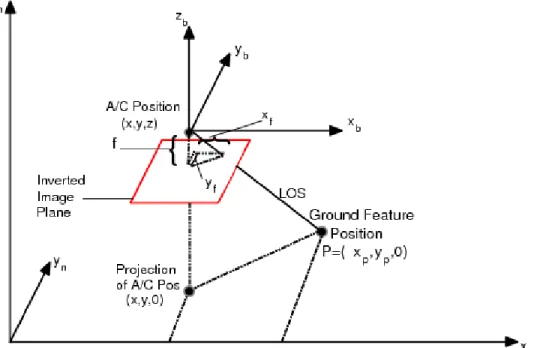
3.3.3 Measurement Equation. The relationship of the inertial position and attitude
of the aircraft to that of the ground object/featurePis x y z = xp yp zp − |RLOS| q x2f +y2f + f2 Cnb xf yf −f (3.25)
wherexf andyf are the projections of the ground feature’s respectivexandycoordinates onto the focal plane of the camera and f is the camera’s focal length - see Figure 3.2. For
the case when the aircraft flies wings level at a constant altitude in the direction of thexn axis and the Euler angles are small, the DCM for relating the body frame to the navigation frame is given in Eq. (3.5). The relationship (3.25) has the appearance of three equations but in fact has the strength of two independent equations. The first two equations in the
Figure 3.2: Measurement Geometry in General Position.
relationship given by Eq. (3.25) are non-linearly dependent on the third. Now, the third equation yields zp−z= |RLOS| q x2f +y2f + f2 0 0 1 Cnb xf yf −f and thus |RLOS| q x2 f +y 2 f + f2 = zp−z 0 0 1 Cn b xf yf −f (3.26)
Substituting Eq. (3.26) into Eq. (3.25) yields the two measurement equations for the three dimensional case: x y = xp yp − zp−z 0 0 1 Cnb xf yf −f 1 0 0 0 1 0 Cnb xf yf −f
Multiplying out the matrices yields x y = xp yp −(zp−z) 1 −f −θxf +φyf xf −ψyf − fθ yf +xfψ+ fφ
and nondimensionalizing such that
xf → xf f , yf → yf f yields x y = xp yp −(zp−z) 1 −1−θxf +φyf xf −ψyf −θ yf +xfψ+φ
Thus, two separate nonlinear measurement equations are obtained
xp−x=−(zp−z) xf −ψyf −θ 1+θxf −φyf (3.27) yp−y=−(zp−z) yf +ψxf +φ 1+θxf −φyf (3.28)
Due to the small angles assumption, the denominator in Eqs. (3.27) and (3.28) can be moved up such that
xp− x≈ −(zp−z)(xf −ψyf −θ)(1−θxf +φyf) (3.29) yp−y≈ −(zp−z)(yf +xfψ+φ)(1−θxf +φyf) (3.30) Since the aircraft is using ground objects to aid its INS, it can be assumed, without loss of generality, that the terrain elevation is known andz = 0. Due to the small values of the
angles, when the former fraction is distributed out, the products of the angles are negligible, yielding
xp−x= z[xf −θ(1+ x2f)+φxfyf −ψyf] (3.31) yp−y=z[yf −θxfyf +φ(1+y2f)+ψxf] (3.32) Next, perturb the states and the measurements
x= xc−δx y=yc−δy z=zc−δz
θ= θc−δθ φ=φc−δφ ψ=ψc −δψ
xp = xpc−δxp yp =ypc−δyp
xf = xf m−δxf yf =yf m−δyf
where the subscriptcindicates the navigation states components provided by the free INS and the subscriptmindicates measured quantities. The calculation of the “nominal” position (xpc,ypc) of a geolocated ground feature will be discussed in the sequel. Inserting the perturbation equations into the measurement Eqs. (3.31) and (3.32) yields
xpc−xc+δx−δxp =(zc−δz)
xf m−δxf −(θc−δθ)(1+x2f m−2xf mδxf +δx2f)
+(φc−δφ)(xf m−δxf)(yf m−δyf)−(ψc−δψ)(yf m−δyf)
Due to the small error in the measurements and the small angles, the products of these terms can be neglected.
xpc−xc+δx−δxp=(zc−δz)
xf m−δxf −(θc−δθ)(1+ x2f m)
+(φc−δφ)xf myf m−(ψc−δψ)yf m
Similarly, in the second measurement equation
ypc−yc+δy−δyp=(zc−δz) yf m−δyf −(θc−δθ)(xf m−δxf)(yf m−δyf)+(φc−δφ) (y2f m−2yf mδyf +δy2f)+(ψc−δψ)(xf m−δxf) =(zc−δz) yf m−δyf −(θc−δθ)xf myf m+(φc−δφ)(1+y2f m) +(ψc−δψ)xf m
Moving all the error terms to the Right Hand Side (RHS) of the equation and all the non-error terms to the Left Hand Side (LHS) yields
xpc−xc−zc[xf m−θc(1+x2f m)+φcxf myf m−ψcyf m]= −δx−δz[xf m−θc(1+x2f m)+φcxf myf m−ψcyf m] +δθ(1+x2f m)zc−δφxf myf mzc+δψyf mzc+δxp−zcδxf (3.33) and ypc−yc−zc[yf m−θcxf myf m+φc(1+y2f m)+ψcxf m]= −δy−δz[yf m−θcxf myf m+φc(1+y2f m)+ψcxf m] +δθxf myf mzc−δφ(1+y2f m)zc−δψxf mzc+δyp−zcδyf (3.34)
Finally, nondimensionalizing such that
xp → xp h yp → yp h zp → zp h,
we also note that the nominal nondimensional altitude isz= 1. In addition, for the purpose of covariance and Kalman Filtering analysis, set all of the calculated and measured values on the RHS equal to the nominal/true values. This causes all of the angles to go to zero, simplifying the measurement Eqs. (3.33) and (3.34). Also, on the RHS setxf m := xf and yf m:= yf, where, in view of the nondimensionalization, and since in the KF
mechanization in each measurement epochtis the time elapsed from the beginning of the epoch, xf = xp−t, yf = yp- see Figure 3.1. Hence, for the first ground object,
xf1(t)=1−t, yf1(t)=yp1and for the second ground objectxf2(t)=2−t, yf2(t)=yp2. Thus, Eqs. (3.33) and (3.34) yield the linearized measurement equations
xpc−xc−zc[xf m−θc(1+ x2f m)+φcxf myf m−ψcyf m]=
−δx− xfδz+δθ(1+x2f)−xfyfδφ+yfδψ+δxp−δxf
(3.35)
and
ypc−yc−zc[yf m−θcxf myf m+φc(1+y2f m)+ψcxf m]=
−δy−δzyf + xfyfδθ−δφ(1+y2)−xfδψ+δyp−δyf
Hence, the time dependent observation matrixH(l) during a measurement epoch with one unknown ground feature is
Hu(l)= −1 0 0 −1 −xf −yf 0 0 0 0 0 0 −xfyf −(1+y2f) 1+x2 f xfyf yf −xf 0 0 0 0 0 0 0 0 0 0 0 0 1 0 0 1 T (3.37)
where the subscriptuindicates that the position of the ground object being tracked is unknown. The nondimensional measurement error is [δxf, δyf]T.
Since, for the sake of observability [9], in each measurement epoch two ground objects will be tracked, there will be two subscripts 1 and 2. The first corresponds to the ground object that is closer to the aircraft and the second to the ground object that is further away. In the first measurement epoch it is assumed that both ground objects are
known. If both ground objects are known, the observation matrix is Hkk(l)= −1 0 −1 0 0 −1 0 −1 −xf1 −yf1 −xf2 −yf2 0 0 0 0 0 0 0 0 0 0 0 0 −xf1yf1 −(1+y2f1) −xf2yf2 −(1+y 2 f2) 1+x2f1 xf1yf1 1+ x2f2 xf2yf2 yf1 −xf1 yf2 −xf2 0 0 0 0 0 0 0 0 0 0 0 0 0 0 0 0 0 0 0 0 0 0 0 0 T (3.38)
where the subscriptk indicates that the position of the ground object is known. In the second measurement epoch a new ground feature is acquired so that in the field of view of the camera there is one known and one unknown ground object. When there is one known
and one unknown ground object, the observation matrix is Hku(l)= −1 0 −1 0 0 −1 0 −1 −xf1 −yf1 −xf2 −yf2 0 0 0 0 0 0 0 0 0 0 0 0 −xf1yf1 −(1+y2f1) −xf2yf2 −(1+y 2 f2) 1+x2f1 xf1yf1 1+x2f2 xf2yf2 yf1 −xf1 yf2 −xf2 0 0 0 0 0 0 0 0 0 0 0 0 0 0 0 0 0 0 0 0 0 0 0 0 0 0 1 0 0 0 0 1 T (3.39)
Finally, starting at measurement epoch three when neither ground object’s position is known, the observation matrix
Huu(l)= −1 0 −1 0 0 −1 0 −1 −xf1 −yf1 −xf2 −yf2 0 0 0 0 0 0 0 0 0 0 0 0 −xf1yf1 −(1+y2f1) −xf2yf2 −(1+y 2 f2) 1+ x2 f1 xf1yf1 1+x 2 f2 xf2yf2 yf1 −xf1 yf2 −xf2 0 0 0 0 0 0 0 0 0 0 0 0 0 0 0 0 0 0 0 0 0 0 0 0 1 0 0 0 0 1 0 0 0 0 1 0 0 0 0 1 T (3.40)
Two ground objects,P1 andP2 are tracked. The measurementszgiven to the Kalman Filter during thenthmeasurement epoch at each time step,l=1,2=L, are generated from
the LHS of Eqs. (3.35) and (3.36) as z= xp1c−xc−zc(xf m1−θc(1+x2f m1)+φcxf m1yf m1−ψcyf m1) yp1c−yc−zc(yf m1−θcxf m1yf m1+φc(1+y2f m1)+ψcxf m1) xp2c−xc−zc(xf m2−θc(1+x2f m2)+φcxf m2yf m2−ψcyf m2) yp2c−yc−zc(yf m2−θcxf m2yf m2+φc(1+y2f m2)+ψcxf m2) (3.41) where xf1(t)=1−t, xf2(t)=2−t, t =l∆T, 1≤ l≤ L and xf m1 =xf1(t)+ξ1, xf m2 =xf2(t)+ξ2, ξ1 ∼ N(0, σ2), ξ2 ∼N(0, σ2), yf m1 =yf1+η1, yf m2 =yf2+η2, η1 ∼ N(0, σ2), η2 ∼N(0, σ2)
whereσ= 13×10−3 (for a 9 mega pixels camera with an aspect ratio of 1). The calculated navigation state is output by the free INS and given by
xc = xF =x+δxF
wherexis the true (nondimensional) navigation state given by
x=[ t 0 1 1 0 0 0 0 0 ]T
andδxFis the navigation state error of the free INS. Thus, the sequenceδxF is obtained as
follows: δxF(l+1)= AadδxF(k), δxa(0)= δP(0) δV(0) δΨ(0) δf(0) δω(0) 15×1
l= 0, . . . ,LN−1 where (δP(xb)(0), δP(yb)(0), δPz(b)(0)∼ N(03×1,1×10−6I3) (δV(xb)(0), δV(yb)(0), δVz(b)(0)∼ N(03×1,1×10−16I3) (δΨ(φb)(0), δΨ(θb)(0), δΨ(ψb)(0)∼ N(03×1,1×10 −8I 3) (δfx(b)(0), δfy(b)(0), δfz(b)(0))∼ N(03×1, σ2aI3) (δω(xb)(0), δω(yb)(0), δωz(b)(0))∼ N(03×1, σ2gI3)
During a measurement epochxp1c, xp2c,yp2c, andyp2cwhich feature in measurements zgiven to the KF are held constant. At the end of the measurement epoch they are updated for the next measurement epoch. They are calculated according to Tables B.1 - B.3 in Appendix B.
3.3.4 Synthesis of the Measurement Sent to the KF in Epoch n. In epoch 1,
xp1c =1,yp1c =−yp, and xp2c = 2,yp2c =yp. In epoch 2,xp1c =2,yp1c = yp.
Consider measurement epochn, 3≤n≤ N,N=360. In total,n+1 ground features are used.n−1 new ground features are geolocated.
The meaning ofx(pcn)andy( n)
pc used during epochn≥2 to calculate the measurement given to the KF - we refer to Eq. (3.41): they are kept constant during the measurement epoch (n) and were calculated at the conclusion of epoch (n−1) using
Eqs. (3.27) and (3.28) and setting thereinzp≡ 0:
x(pn2)c = x+z xf −ψyf −θ 1+θxf −φyf (3.42) y(pn2)c =y+zyf +ψxf +φ 1+θxf −φyf (3.43)
Since the scenario considered is wings level flight at constant altitude, in Eqs. (3.42) and (3.43) set
x=n−1+δxF|n−1−δxˆ |n−1, y=δyF|n−1−δyˆ|n−1, z=1+δzF|n−1−δzˆ|n−1, ψ=δψF|n−1−δψˆ |n−1, θ=δθF|n−1−δθˆ|n−1, φ=δφF|n−1−δφˆ |n−1
and since at the end of an epoch the newly acquired ground feature’sxf =2, yf = ±yp, in Eqs. (3.42) and (3.43) set
xf =2+ξ, ξ ∼ N(0, σ2), yf =±yp+η, η∼ N(0, σ2) where σ= 1 3 ×10 −3, δxF|n−1 ≡δxF((n−1)L), δyF|n−1 ≡δyF((n−1)L) whereas ˆ δx|n−1 ≡δxˆ (n−1) (L), δyˆ|n−1 ≡δyˆ (n−1) (L)
and the same applies to the navigation statesz, ψ, θ, φ. In addition, at the end of the measurement epochn−1, set
x(pn1)c :=x(pn2−c1)−δxˆ (pn2−1)(L), y(pn1)c :=y(pn2−c1)−δyˆ(pn2−1)(L),
Also, at the end of the measurement epoch 1 set
x(2)p1c =2, y(2)p1c =0
Also, during measurement epochn, at timel, in Eq. (3.41)
xc =t+δxF(t), yc =δyF(t), zc = 1+δzF(t), θc =δθF(t), φc =δφF(t), ψc = δψF(t) where t=n−1+ ∆T ∗l, l=1,· · · ,L, ∆T =1/L and xf1m = xf1+ξ1, ξ1 ∼ N(0, σ2), xf2m = xf2+ξ2, ξ2 ∼ N(0, σ2), yf1m =±yp+η1, η1 ∼ N(0, σ2), yf2m =∓yp+η2, η2 ∼ N(0, σ2) where, during the measurement epoch (n)
xf1= 1−l∆T, xf2= 2−l∆T, l=1,· · · ,L
3.4 Performance of Aided INS
The performance of the aided INS is evaluated for the nominal scenario described in Section 3.2 and illustrated in Figure 3.3. The aircraft is flying wings-level, at a constant speed with ground features spaced at one kilometer apart. The first two ground features are known and the aircraft starts one kilometer behind the first ground feature. In the observation matricesH,
If ground features are arranged in a straight line on the positivexn axis, then in theH matrix
yf1(t)= yf2(t)= 0
However, if the ground features are laterally staggered at equal distanceypabout the positivexn axis, then in theHmatrix
yf1(t)=yp yf2(t)=−yp
Aircraft using measurement
Aircraft geo-locates unknown ground object Aircraft stops using ground object
Zi
Xi
Known Ground Points Unknown Ground Points
Pos(t3) Pos(t2) Pos(t1) Pos(t4) Xp3 Xp4 Xp1 Xp2 Pos(t0) 1 1 1 1 2 2 2
Epoch 1 Epoch 2 Epoch 3
Xp1 Xp2
Epoch 1
Epoch 2
Epoch 3
Figure 3.3: In the first measurement epoch the two ground objects’ position are known, but in the second measurement epoch there is one known and one unknown ground object, where the unknown object’s position was estimated by the aircraft at the end of the first epoch. From epoch 3 onward both ground objects’ locations are estimated using the aircraft’s navigation state at the end of the preceding epoch and therefore are not exactly known.
3.4.1 Initialization of the KF. In the first measurement epoch the Kalman Filter is initialized according to Eq. (3.44)
(δˆx+a(0))(1)= 015×1 (3.44) while the covariance matrix is initialized as (P(0))(1) by usingPas in the equation
following Eq. (3.24) where it is assumed that the position, velocity, and orientation are known with an uncertainty ofa= 1×10⁻⁶,b=1×10⁻¹⁶, andc= 1×10⁻⁸, respectively as in, Eq. (3.45). (P(0))(1) = A 0 0 0 0 0 B 0 0 0 0 0 C 0 0 0 0 0 D 0 0 0 0 0 E 15×15 (3.45) where A=diag(a,a,a) B=diag(b,b,b) C =diag(c,c,c) D=diag(σ2a, σ2a, σ2a) E =diag(σ2g, σ2g, σ2g)
The superscripts in (δˆx+a(0))(1) and (P(0))(1)represents the epoch number (epoch 1 in this case). The three accelerometer and the three gyroscope set are of the same quality: the random biases in the sensors are
δfxb∼ N(0, σ2a) δfyb ∼N(0, σ2a) δfzb ∼ N(0, σ2a) δωb x ∼ N(0, σ 2 g) δω b y ∼N(0, σ 2 g) δω b z ∼ N(0, σ 2 g)
In each measurement epoch the KF is re-initialized. Since in measurement epochn,n≥ 2, one navigates offa newly acquired ground feature, the KF is being re-initialized as