R E S E A R C H
Open Access
The effect of spatial structure of forests
on the precision and costs of plot-level
forest resource estimation
Henrike Häbel
1, Mikko Kuronen
1, Helena M. Henttonen
1, Annika Kangas
2and Mari Myllymäki
1*Abstract
Background: We investigated how the precision and costs of forest resource estimates for sample plots of different type and size depend on the spatial structure of forests and jointly studied the effects of tree density and size distribution. Statistically thinking, the trees in a forest can be regarded as a point pattern. Based on the spatial properties of the point pattern, we classified the forests into clustered, random, and regular. We used empirical data from 396 mapped forest plots from Finland. The variance of the unbiased Horvitz-Thompson estimator and expected costs of the basal area and tree density estimation were calculated for 99 different sample plots of different type and size in each of the 396 forest plots. Further, we considered the estimation of the change between two time points for a subset of the data.
Results: The precision and expected cost depended on the tree size distribution and spatial pattern of trees. While large sample plots are advisable for clustered forests or the monitoring of young forests with small trees, we see potential for measuring smaller sample plots in regular forests. The choice of sample plot was more important in clustered forests, where also the variability of the expected costs was higher.
Conclusions: If the spatial structure of forests could be predicted accurately and precisely prior to field measurements, for instance from remote sensing data, the precision of forest inventories could potentially be improved or costs decreased by allowing the sample plot size and type to vary from one forest stand to another. When using a compromise sample plot over a large region and a long inventory rotation, optimizing the sample plot for one time point ignores possible changes in forest structures caused by changes in forest management practices.
Keywords: Concentric circular plot, Expected costs, Fixed radius plot, Forest inventory, Horvitz–Thompson estimator, Relascope plot, Sample plot, Spatial pattern of trees, Spatial structure
Background
Typically, a sampling-based national forest inventory (NFI) is carried out to provide statistics, for example for national or regional forest programs, sustainability assessments, investment calculations for forest indus-try, and reporting to international conventions (Tomppo et al.2010). Forest management inventories (FMI), on the other hand, are carried out to support forest owners in their strategic planning as well as aid decision making concerning harvests and silvicultural measures.
*Correspondence:[email protected]
1Natural Resources Institute Finland (Luke), Latokartanonkaari 9, FI-00790 Helsinki, Finland
Full list of author information is available at the end of the article
NFIs are based on a set of field plots, for instance in Finland about 15 000 plots are measured each year (Kangas et al.2018) totaling to 75 000 plots during each five year inventory rotation. In recent years the forest manage-ment inventories have been carried out using airborne laser scanning (ALS) data and field plots (e.g. Næsset (2004)). The field plots used may be the NFI field plots or plots measured as a separate measurement campaign. Thus, the field plot measurement is a large investment, and it is important to make it as cost-efficiently as possible.
In NFI, the inventory design is optimized in the sense that we wish to have the highest accuracy and precision given a fixed budget or we wish to have the lowest cost
for a given precision (Päivinen1987). In a cluster design, that entails selecting the number of clusters or distance between them, the number of plots in each cluster and the distance between them, and the type and size of plots within each cluster. Optimization is possible, if we make assumptions concerning the population (Mandallaz2007). In an analytic setting, we need to be able to anticipate the between-plot variance (Mandallaz and Ye1999).
Defining optimal sample plot size and type analytically would require that we can anticipate the effects of the plot size and type on the between-plot variance. If the expected between-plot variation could be expressed as a function of plot size (see Zeide (1980)) the optimal plot size could be calculated analytically. The optimal size, however, also depends on the size distributions of the forest stands as well as on the spatial patterns of trees.
While some factors affecting the accuracy and preci-sion can be accounted for analytically, other aspects like the spatial structure of forests are more complicated. The analytic calculations usually assume a random pattern (Mandallaz2007). In Finland, however, regular patterns of trees have been observed more commonly (57%) than ran-dom (25%) and clustered (18%) patterns (Tomppo1986). Therefore, the optimal plot is typically addressed using simulation (e.g. Henttonen and Kangas (2015)).
In this study based on field data from different types of forests, we compared the precision of the basal area and tree density estimation and costs for various sam-ple plots of different type and size. We used the unbiased Horvitz-Thompson estimator to estimate the basal area and tree density and obtained its variance by integrating over the forest plot. The resulting standard deviation and corresponding costs of various sample plots were investi-gated with respect to the spatial structure of forests and other stand variables such as tree density, basal area and diameter distribution that are potentially correlated with the spatial structure (see e.g. Tomppo (1986) p. 40 ff.). By classifying our data, we studied how the spatial struc-ture of forests and other stand variables affect precision and costs of different sample plots. Further, we examined the effect of small trees on the spatial structure, precision and costs.
Methods Materials
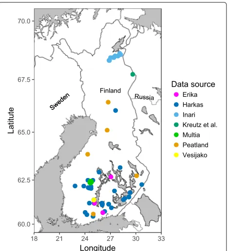
We used data of tree locations and diameters measured at 1.3 m (dbh) from different types of forest stands, including experiments of uneven-aged forest management and thin-nings from below resulting in different spatial patterns of trees. Also data from natural forests and peatlands were included. The total number of forest plots from different data sources was 396 (Fig.1). In order to distinguish this data from the sample plots, they are henceforth referred to as forest plots.
Fig. 1Locations of 396 forest plots from different Finnish data sources
Erika
The Erika data set consists of 21 experimental plots of 40 m×40 m in managed, uneven-aged Norway spruce dominated forests at five locations in southern Finland (Eerikäinen et al.2014). Between 1991 and 2012, the plots were measured usually four to five times with five years’ intervals, recording the locations, tree species, and size characteristics (dbhand height) of all trees≥10 cm tall. Trees withdbh≥0.1 cm were included in our calculations. Only the fourth measurement of each plot was included in our main study. These measurements were taken either in 2007 or 2012. From one plot with only two measurements, the data from 1992 was used.
Harkas
exactly equal to those presented in earlier reports. The median area of the plots was 1004 m2(range 788 m2- 2460 m2). The minimumdbhin the Harkas measurements was 4.5 cm.
Inari
The Inari data setconsists of 18 forest plots of size 50 m×50 m measured on the locations of plots from the 8th Natio-nal Forest Inventory in northernmost Finland (Henttonen and Kangas 2015). The coordinates (tachymeter mea-surement) anddbh of all trees with dbh ≥2.5 cm were recorded.
Multia
The Multia data setconsists of 30 field plots of size 32 m
×32 m measured in 2014 in Multia and Keuruu, southern Finland (Tomppo et al.2016). These data were collected for validation of a remote-sensing based forest resource estimation. Therefore, plots were subjectively located to young thinning stands, advanced thinning stands and mature stands. The coordinates anddbhs of trees withdbh ≥2.5 cm were measured using Sonar caliper.
Various additional data sets
The Various additional datasets consist of large plots measured in different types of forests. Data from Vesijako, southern Finland, comprises two plots of size 100 m
×100 m and 70 m ×130 m. The plots were located in mixed coniferous advanced thinning stands dominated by Norway spruce and Scots pine, respectively. The coordi-nates (tachymeter measurement) and size characteristics (dbhand height) of all trees were recorded. The smallest observeddbhin these plots was 5.7 cm.
The data from Kreutz et al. (2015) was collected from Värriö Strict Nature Reserve in northeastern Finland and it consists of three plots of size 300 m×40 m located in natural forests at different successional stages. In measur-ing treedbhs they were rounded to the closest cm. The minimumdbhwas 1 cm.
Hökkä et al. (2008) collected mapped tree data from seven Scots pine dominated stands growing on drained peatlands in different parts of Finland. We used their data from a total of 10 plots in five stands. Similarly to the processing of Harkas data set, we left out some parts of the data because of missing or unclear plot corner or tachymeter location measurements and the plot areas were thus not equal to the report of Hökkä et al. (2008). The median area of plots in our calculations was 6392 m2(range 1604 m2- 15620 m2). The minimumdbhwas 4.5 cm.
Sample plot types and sizes
We considered 99 different sample plots, including differ-ent specifications for the circular fixed radius determining the overall size, relascope and circular concentric plots specifying the type as follows:
(i) Fixed radius plots with the radiusrmax=3, 4,. . ., 11
m in which all trees above a certaindbh are measured (9 different plots).
(ii) Relascope plots with the maximum radius
rmax=3, 4,. . ., 11m and basal area factors q=1, 1.5, 2, 2.5, 3(45 different plots). A tree is included in the sample plot if its distance to the sample plot center is at mostmin(rmax, 50dbh/√q)
(see Tomppo et al. (2011, p. 25 f.) for more details). (iii) Concentric plots with radii(r1,rmax)=(1, 3),(2, 4),
(3, 5),(4, 6),(5, 7),(5, 8),(6, 9),(6, 10),(7, 11)m for the two circles where the trees with thedbh smaller than 5, 7.5, 10, 12.5, 15 cm are measured only from the smaller circle with radiusr1(45 different plots).
Precision of forest resource estimation
We assumed that the sample plot locationsis chosen uni-formly randomly from the observed forest plot window
W ⊂ R2 and that the forest characteristic Y is esti-mated using the unbiased Horvitz–Thompson estimator (Horvitz and Thompson1952)
ˆ
Y(s)= 1 |W|
n
i=1 Ii(s)Yi
πi
, (1)
where n is the finite number of observed trees in the observation windowWof the forest plot,Ii(s)is the indi-cator that treeiis in the sample plot centered ats, Yi is the characteristic of treei,πiis the inclusion probability of treei, and|W|denotes the forest plot area. We considered the estimation of the tree density measured in number of stems per hectare (Yi =1) and the basal area per hectare
Yi=π(dbhi/2)2
.
We measured the precision of the forest resource esti-mation by the variance of the estimator (1). Based on Theorem 4.2.1. from Mandallaz (2007), the variance is
V[Yˆ(s)]= 1
|W|2
n i=1 n j=1
YiYj(πij−πiπj) πiπj
, (2)
whereπijis the inclusion probability for the pair of treesi andj, given by
πij=E[Ii(s)Ij(s)]= |
B(xi,ri)∩B(xj,rj)∩W|
|W| , (3)
wherexiis the location of treei,riis the inclusion radius for tree i given by the sample plot type and size, and
We further considered the estimation of the change from a time point 1 to time point 2 for the Erika data with measurements repeatedly over time, and estimated the change simply as the difference of the estimates at the two time points, Yˆ(2)(s) − ˆY(1)(s). The formula for the variance of the difference is
V[Yˆ(2)(s)− ˆY(1)(s)]=V
ˆ Y(2)(s)
+V
ˆ Y(1)(s)
−2Cov
ˆ
Y(1)(s),Yˆ(2)(s) , (4) where Cov ˆ
Y(1)(s),Yˆ(2)(s)
= | 1 W|2
n1 i=1 n2 j=1
Yi(1)Yj(2)(π1i2j−π1iπ2j) π1iπ2j
,
(5)
where 1iand 2jrefer to treeiat time point 1 and treejat time point 2, respectively.
Costs for the comparison of sample plot types and sizes We assumed that the cost (time in minutes) to measure treeiin the sample plot of certain type and size was
ci=0.5·1(s∈B(xi,ri)∩W)
+0.5·1(s∈[B(xi, 1.1ri)\B(xi, 0.9ri)]∩W), (6)
where s is the sampling location andri is the inclusion radius of treei. Thus, we assumed simply a fixed cost per measured tree (0.5 min) and an additional cost per border-line tree (0.5 min). A tree was defined to be a borderborder-line tree if its distance from the sample location was between 0.9riand 1.1ri. Given the single tree cost (6), the expected cost for measuring the sample plot is
E n
i=1 ci=
n
i=1
Eci, (7)
where
Eci=0.5|
B(xi,ri)∩W| |W|
+0.5|[B(xi, 1.1ri)\B(xi, 0.9ri)]∩W|
|W| .
Similarly as the variance (2), the expected cost (7) was calculated for each sample plot in each forest plot.
The expected cost for trees of the sample plot in a size classDk=[dk,dk+1),k=1,. . .,K, is
E n
i=1
ci1(dbhi ∈Dk)= n
i=1
1(dbhi ∈Dk)Eci.
Classification of forest structure
In order to study the effect of spatial structure of forests on the precision and costs of different sample plots, the forest plots were divided into different groups of similar stand variables.
For the classification of the spatial structure of a for-est plot, tree locations (at stem center) are mathematically expressed as point patterns(x1,. . .,xn)with a finite num-ber ofntrees observed on a forest plot windowW. Each point pattern is analyzed as a realization of a point process
X, which is assumed to be translation and rotation invari-ant. In what follows, the terms point and tree location can be used interchangeably. Likewise, the intensity λof the point process is equal to the tree density, albeit per m2.
The tree locations were divided into clustered, random and regular patterns by utilizing the L-function, which is the variance stabilizing transformation of Ripley’s K -function (Chiu et al.2013, Chapter 4.6) given by
L(r)=
K(r)
π ∀r≥0. (8)
The functionλK(r)gives the expected number of points ofX within a circleB(o,r) around a typical pointoand radiusr(in m) without countingoitself given that there is a point ofXino.
In the completely spatially random (CSR) case with no interaction between the points,L(r)−r=0 for allr≥0. This fact can be used in a test for CSR based on the test statistic
τ =max
r≤rt |L(r)−r| (9)
with Ripley’s isotropic edge corrected estimatorL. The CSR hypothesis can be rejected at a 5% significance level if
τ >1.45
√ |W|
n (10)
(Chiu et al. 2013, pp. 57 f., 139 ff.). Due to size limita-tions of some forest plots in the Harkas data, distances up to rt = 5 m were taken into account for a short range classification.
For the analysis, the statistical software R version 3.4.4 (Core Team 2018) was used together with the package
spatstat(Baddeley et al.2015).
Results
Table 1Average tree density (standard deviation) in trees/ha, average basal area weighted meandbhin cm (standard deviation), average basal area (standard deviation) in m2/ha, and number of clustered, random, and regular plots for the Erika (21 plots), Harkas (312 plots), Inari (18 plots), Multia (30 plots), and various other data sources (15 plots)
Tree Min Mean Basal Structure
density dbh dbhBA area Clustered Random Regular
Erika 1571 (630) 0.1 26 (3) 23 (4) 15 4 2
Harkas 949 (536) 4.5 23 (4) 30 (9) 2 2 308
Inari 711 (392) 2.5 18 (6) 8 (5) 12 4 2
Multia 2855 (1866) 2.5 15 (6) 23 (8) 10 2 18
Various 1000 (386) 0.5-5.7 16 (7) 17 (8) 6 0 9
and mean dbh. The Harkas data including the thinning experiments have regular tree patterns, a lower average tree density, and the largest basal area. The Inari data with a minimumdbh of 2.5 cm have relatively few trees and appear mostly clustered, whereas the Multia data with the same minimumdbh, but higher tree density, have both clustered and regular patterns. In contrast to Tomppo (1986), where smaller forest plots where considered, only 12 forest plots (3%) were classified as random. This small proportion of random forests results from large forest plots of this study that facilitate the detection of clustering and regularity due to more observations.
Given the classification according to spatial structure, the forest plots were partitioned according to stan-dard deviation ofdbh, basal area and tree density using the recursive partitioning function implemented in the
rpartR package (Therneau et al.2017). We concluded
from the partitioning for forest structure that clustered patterns had a larger dbh range than regular patterns, whereas regular patterns tended to have larger trees with about the same size. Consequently, a grouping with respect todbhstandard deviation was not informative for this study since one group would mainly contain clustered and the other mainly regular forests. In our data, all forest plots with a tree density≥3214 trees/ha were classified as clustered.
Based on the partitioning, each forest plot was classified as a plot with small (< 9.8 m2/ha), medium (in [9.8,32) m2/ha) or large (≥ 32 m2/ha) basal area. We further defined different development classes also taking Tomppo et al. (2011, Table 2.17) into consideration. The result-ing development classes are based on the mean basal area weighteddbh(dbhBA) and tree density:
• seedling stand : meandbhBA<8cm or density
>3214trees/ha,
• young stand : meandbhBAin [8,26] cm and density in
(1500,3214] trees/ha,
• advanced stand : meandbhBAin [8,26] cm and
density in (500, 1500] trees/ha,
• mature stand : meandbhBA>26cm or tree density ≤500trees/ha.
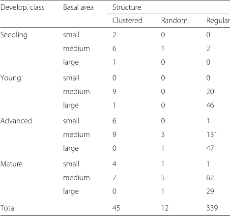
Seedling stands tend to be clustered and forest plots with large basal area regular (Table2).
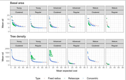
The effect of spatial structure on precision and costs In order to study the effect of clustered and regular pat-terns on precision and costs of different sample plot types and sizes, we focused on forest plots with medium basal area ([ 9.8, 32)m2/ha) not belonging to the seedling class. We selected this group of forest plots as it contains both clustered and regular patterns with more than two obser-vations each. Then, we compared the mean standard deviation of the estimator (1) and mean expected costs (7) per forest structure group and sample plot type and size (Fig.2). The higher the tree density (younger devel-opment classes), the lower the precision of the estimated tree density and the bigger differences between the dif-ferent sample plot types both for clustered and regular forest plots. The differences between different develop-ment classes and different sample plot types in the basal
Table 2Number of plots per group after classification with respect to development class and basal area (small:<9.8, medium: [ 9.8, 32), large:≥32 m2/ha), and spatial structure of forests
Develop. class Basal area Structure
Clustered Random Regular
Seedling small 2 0 0
medium 6 1 2
large 1 0 0
Young small 0 0 0
medium 9 0 20
large 1 0 46
Advanced small 6 0 1
medium 9 3 131
large 0 1 47
Mature small 4 1 1
medium 7 5 62
large 0 1 29
Fig. 2Precision versus expected costs for different fixed radii (maximum radius between 3 and 11 m), relascope (basal area factors from 1 to 3), and concentric plots (dbhlimit from 5 to 15 cm) sample plots for the estimation of basal area and tree density in clustered and regular forest plots of different development classes (see text for description). The precision has been measured by the standard deviation (sd) of the respective estimator (1) averaged over the forest plots. This is a zoomed view and some values have been cut off
area estimation were smaller, largest differences between the sample plot types occurring for clustered patterns and in the youngest development class. In any case, both for clustered and regular forest plots, the relascope sample plots appeared to be the most efficient choice to esti-mate basal area. On the contrary, they were unfeasible for the tree density estimation. In this case, the fixed radius plots seems to be the best design. In general, the precision was lower in clustered forests than in regular forests. Increasing the maximum radiusrmax (increasing the costs) further led to a more pronounced improvement of precision for clustered than for regular patterns (see also Table3).
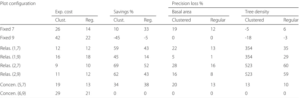
In a more detailed study, we focused on eight different sample plots with two different maximum radii, namely 7 and 9 m. For the relascope plot we considered the basal area factors 1 and 2 for each case. The inner radii of the concentric plots with these maximum radii were 5 and 6 m, respectively, and thedbhlimit was set to 10 cm. We compared the average expected costs for clustered and regular patterns (Table3) and found that the fixed radius plots were almost twice as expensive for clustered than for
Table 3Average expected costs (time in minutes) for measuring eight different sample plots, cost savings (in %), and loss of precision (in %) determined by the increase in standard deviation of the estimator for basal area and tree density
Plot configuration Precision loss %
Exp. cost Savings % Basal area Tree density
Clust. Reg. Clust. Reg. Clustered Regular Clustered Regular
Fixed 7 26 14 10 33 19 12 -5 6
Fixed 9 42 22 -45 -5 0 0 -18 -3
Relas. (1,7) 12 12 59 43 22 13 354 35
Relas. (1,9) 16 18 45 14 5 1 354 29
Relas. (2,7) 9 10 69 52 28 16 523 60
Relas. (2,9) 11 12 62 43 16 8 523 59
Concen. (5,7) 19 13 34 38 20 13 13 10
Concen. (6,9) 29 21 0 0 0 0 0 0
The values are presented separately for clustered and regular patterns. Percentages are calculated in reference to the concentric plot with a 9 m maximum and a 6 m inner radius. For all concentric plots, trees with adbh<10 cm were only measured in the inner circle
basal area estimation among the evaluated sample plots seems to be the relascope plot with a maximum radius of 9 m and the basal area factor 1, but even the basal area factor 2 gave reasonable precision. For tree density, it appeared worth taking the fixed radius plot with a maximum radius of 7 m into account instead of the concentric plot with a 9 m maximum radius. Not only can costs be saved, but there is even an improvement in precision for clustered patterns.
We also studied the distribution of costs and precision among the clustered and regular forests for the selected eight sample plots with boxplots (Fig.3). In general, the precision was higher (lower standard deviation of the esti-mators) for regular patterns than for clustered. Further, the variability was lower for regular than for clustered patterns in all cases, especially for the precision of the relascope estimation of tree density and expected costs of the fixed radius plots. The variability of the basal area estimation appears similar for all sample plots for either clustered or regular forests. Relascope plots had the small-est cost variability, but they showed a large variability in precision for tree density estimation.
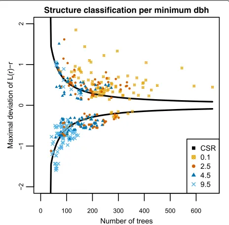
The effect of minimumdbhon spatial structure and change
estimation
We studied the effect of the minimum dbh on the spa-tial structure classification and the estimation of change in tree density between consecutive time measurements using all 98 measurements from the Erika data source. The spatial structure classification depended on the min-imum dbh of the trees measured in the forest plots, where with a minimumdbh of 0.1 cm, most of the pat-terns were classified as clustered (Fig. 4). There was a clear shift towards more regular patterns with increasing
dbhlimit.
The minimum dbh also had an effect on precision and costs in the change estimation, where with increas-ing minimum dbh, precision increased while cost and cost variability decreased (Fig. 5). Consequently, mini-mum dbhs of 2.5 or 4.5 cm decreased the costs con-siderably in comparison to the 0.1 cm limit, but the patterns were still clustered (Fig. 4). With a minimum
dbh of 9.5, the locations of the measured trees mostly formed a regular pattern, where all sample plot types included almost the same trees (Fig.5). If the main inter-est is to study the development of young forinter-ests, e.g. changes in small trees (with dbh ≤ 9.5 cm), the tree density is typically more important than the basal area. In order to minimize the variance (4) of the estimated change such studies should be based on large fixed radius plots (Fig.5).
Discussion
Fig. 3Boxplots of precision measured by the standard deviation (sd) of the estimator (1) and costs for eight sample plots with maximum radii 7 and 9 m, basal area factors 1 and 2, and inner radii 5 and 6 m, where trees with adbh<10 cm were only measured in the inner circle. This is a zoomed view and some values have been cut off
number of trees and borderline trees are the main factors affecting the costs.
If the spatial structure of forests could be predicted prior to field measurements, for instance from remote sensing data (see e.g. Packalen et al. (2013); Pippuri et al. (2012); Häbel et al. (2018)), it would in principle be possible to let the sample plot size and type vary from a forest to another. However, in the current inventories, the same sample plot is used over the whole inventory region and, thus, a compromise solution is needed. Another aspect is the
Fig. 4Maximal deviation of the centeredL-function from zero for all 98 measurement of the 21 Erika forest plots and for different minimumdbhranging from 0.1 to 9.5 cm. The solid black lines give the classification bounds for the CSR case, where values above the upper bound correspond to patterns classified as clustered and values below the lower bound to regular patterns
For selecting a sample plot for an operational NFI, we need to balance the measurements of small trees so that the RMSE of tree density is acceptable while the plot design is cost-efficient and robust. In order to produce an optimal and operational plot, we could introduce a
probabilistic budget constraint, such that P(time used for measuring a cluster of x plots <8 h) > p, and minimize the RMSE of tree density subject to that con-straint. In this approach, the parameters to be defined are the number of plots within a cluster and the required probabilityp.
Measurements from forest plots are not only used in inventory calculations, but they are also used as auxiliary variables in model-assisted stand variable estimation. In FMIs, for instance, the collected data are used to build a model to predict the forest variables of interest to all pix-els (raster cells) for a map of a certain region of interest. In such a case, the quality of sample plots may be assessed based on the performance of those models. Adnan et al. (2017) studied the effect of sample plot size and stand density on the quality of estimation of tree size hetero-geneity from ALS. Tree size heterohetero-geneity can be related to the spatial structure of forests since regular patterns have a tendency to be even-aged with about the same size for all trees and clustered patterns tend to be uneven-aged or show at least a larger variation in tree size. Adnan et al. (2017) concluded that for a reliable field-based esti-mation the smallest sample plot size required is 6 m, but that plot sizes between 9 and 12 m maximize the cor-relation between field values and ALS metrics. Tomppo et al. (2016) also studied ALS-assisted forest resource esti-mation, but not for the spatial structure. They suggested that a relascope plot with a basal area factor 1 or a con-centric plot with a maximum radius of 9 m and an inner radius of 5.64 m and a lowerdbhlimit of 9.5 cm for the outer circle (used in the Finnish NFI) could be used to
reduce the cost in comparison to a fixed radius plot with a 9 m maximum radius while still being feasible for ALS-assisted inventories. Future studies could assess whether case depended optimal sample plots can be found for remote sensing-assisted inventories.
Conclusions
We classified forests according to spatial structure, tree density and size distribution and found that regular and clustered patterns of trees tend to have different forest characteristics. All in all, it can be concluded that both precision and costs vary depending on the tree density, basal area, diameter distribution, and spatial structure of a forest as well as estimated forest variable. Therefore, there seems to be no obvious overall optimal sample plot.
Today’s forests in Finland are most often regular as a result of the silvicultural methods used since the 1950s, which include forest regeneration most often by clear-cut and planting, or due to thinnings from below in younger forests. The amendments to the Forest Act (2013) allow uneven-aged forest management since 2014. This will slowly increase the proportion of clustered forests. This trend makes the monitoring of the development of small trees even more important than before e.g., for the estima-tion of forest growth and for the predicestima-tion of scenarios for the future development of forests. For these purposes, sample plots which give more weight to small trees than relascope plots, where the inclusion probability is pro-portional todbh2, could be considered. For example, this could be achieved by estimating the inclusion probabili-ties of trees as a function of several tree characteristics (instead of onlydbh2) using data from previous invento-ries. Also step functions, leading to multiple concentric circles with the radii depending on tree characteristics, could be used in practice.
Abbreviations
ALS: Airborne laser scanning; dbh: Diameter at breast height measured at 1.3 m; FMI: Forest management inventory; NFI: National forest inventory; RMSE: Root mean squared error
Acknowledgements
We wish to thank Saija Huuskonen, Hannu Hökkä, Harri Mäkinen, Risto Ojansuu and Erkki Tomppo for providing the data as well as Merja Arola and Ville Pietilä for advice in data processing. The authors would also like to thank Kari T. Korhonen for helpful discussions.
Funding
Henrike Häbel, Mikko Kuronen and Helena Henttonen were financially supported by the Academy of Finland (Project Number 304212) and Mari Myllymäki similarly by the Academy of Finland (Project Numbers 295100 and 306875).
Availability of data and materials
The data is not owned by the authors and cannot be shared. The R code is available upon request.
Authors’ contributions
All authors were involved in planning and conducting the study as well as writing the manuscript. HH conducted the classification, statistical analysis and
most of the manuscript writing. MK did the variance and cost calculations. HMH was responsible for the data management. AK mainly contributed to the background and discussion. MM was the principal investigator of this study, had acquired the funding, and supervised HH and MK. All authors read and approved the final manuscript.
Ethics approval and consent to participate
Not applicable.
Consent for publication
Not applicable.
Competing interests
The authors declare that they have no competing interests.
Author details
1Natural Resources Institute Finland (Luke), Latokartanonkaari 9, FI-00790 Helsinki, Finland.2Natural Resources Institute Finland (Luke), Yliopistokatu 6, 80100 Joensuu, Finland.
Received: 19 November 2018 Accepted: 19 February 2019
References
Adnan S, Maltamo M, Coomes D, Valbuena R (2017) Effects of plot size, stand density, and scan density on the relationship between airborne laser scanning metrics and the gini coefficient of tree size inequality. Can J Forest Res 47(12):1590–1602
Baddeley A, Rubak E, Turner R (2015) Spatial Point Patterns: Methodology and Applications with R. Chapman and Hall/CRC Press, London
Chiu SN, Stoyan D, Kendall WS, Mecke J (2013) Stochastic Geometry and its Applications. 3rd edn. Wiley, Chichester
Core Team R (2018) R: A Language and Environment for Statistical Computing, Vienna.https://www.R-project.org/
Eerikäinen K, Valkonen S, Saksa T (2014) Ingrowth, survival and height growth of small trees in uneven-aged picea abies stands in southern finland. Forest Ecosystems 1:5.https://doi.org/10.1186/2197-5620-1-5
Forest Act (2013).http://www.finlex.fi/fi/laki/kaannokset/1996/en19961093.pdf Häbel H, Balázs A, Myllymäki M (2018) Spatial analysis of airborne laser
scanning point clouds for predicting forest variables. arXiv:1805.08907 [stat.AP].,https://arxiv.org/abs/1805.08907
Henttonen HM, Kangas A (2015) Optimal plot design in a multipurpose forest inventory. Forest Ecosystems 2(1):1–14. https://doi.org/10.1186/s40663-015-0055-2
Hökkä H, Koivusalo H, Ahti E, Nieminen M, Laine J, Saarinen M, Laurén A, Alm J, Nikinmaa E, Klöve B, Marttila H (2008) Effects of tree stand transpiration and interception on site water balance in drained peatlands: experimental design and measurements. In: Farrell C, Feehan J (eds). After Wise Use -The Future of Peatlands, Proceedings of the 13th International Peat Congress, Tullamore, vol. 2. pp 169–171
Horvitz DG, Thompson DJ (1952) A generalization of sampling without replacement from a finite universe. J Am Stat Assoc 47(260):663–685. https://doi.org/10.1080/01621459.1952.10483446
Kangas A, Astrup R, Breidenbach J, Fridman J, Gobakken T, Korhonen KT, Maltamo M, Nilsson M, Nord-Larsen T, Næsset E, Olsson H (2018) Remote sensing and forest inventories in nordic countries - roadmap for the future. Scand J Forest Res 33(4).https://doi.org/10.1080/02827581.2017.1416666 Kreutz A, Aakala T, Grenfell R, Kuuluvainen T (2015) Spatial tree community
structure in three stands across a forest succession gradient in northern boreal fennoscandia. Silva Fenn 49(2):397–412.https://doi.org/10.14214/sf. 1279
Mäkinen H, Isomäki A (2004) Thinning intensity and growth of scots pine stands in finland. Forest Ecol Manag 201(2–3):311–325.http://dx.doi.org/ 10.1016/j.foreco.2004.07.016
Mandallaz D (2007) Sampling Techniques for Forest Inventories. CRC Press, Boca Raton
Mandallaz D, Ye T (1999) Forest inventory with optimal two-phase, two-stage sampling schemes based on the anticipated variance. Scand J Forest Res 29(11):1691–1708
Packalen P, Vauhkonen J, Kallio E, Peuhkurinen J, Pitkänen J, Pippuri I, Strunk J, Maltamo M (2013) Predicting the spatial pattern of trees by airborne laser scanning. Int J Remote Sens 34(14):5154–5165.https://doi.org/10.1080/ 01431161.2013.787501
Päivinen R (1987) Metsän inventoinnin suunnittelumalli. [A planning model for forest inventory, In Finnish]. 11th edn. University of Joensuu publications in Sciences, University of Joensuu, Joensuu
Pippuri I, Kallio E, Maltamo M, Peltola H, Packalén P (2012) Exploring horizontal area-based metrics to discriminate the spatial pattern of trees and need for first thinning using airborne laser scanning.https://doi.org/10.1093/ forestry/cps005
Therneau T, Atkinson B, Ripley B (2017) rpart: Recursive Partitioning and Regression Trees.,.https://CRAN.R-project.org/package=rpart, r package version 4.1-11
Tomppo E (1986) Models and methods for analysing spatial patterns of trees. Communicationes Instituti Forestalis Fenniae 138
Tomppo E, Gschwantner T, Lawrence M, McRoberts RE (eds) (2010) National Forest Inventories. Pathways for Common Reporting. Springer, Heidelberg Tomppo E, Heikkinen J, Henttonen HM, Ihalainen A, Katila M, Mäkelä H,
Tuomainen T, Vainikainen N (2011) Designing and Conducting a Forest Inventory - case: 9th National Forest Inventory of Finland. Springer, Dordrecht
Tomppo E, Kuusinen N, Mäkisara K, Katila M, McRoberts RE (2016) Effects of field plot configurations on the uncertainties of ALS-assisted forest resource estimates. Scand J Forest Res 32(6):488–500.https://doi.org/10. 1080/02827581.2016.1259425