Research Article
Robust Color Image Superresolution:
An Adaptive M-Estimation Framework
Noha A. El-Yamany and Panos E. Papamichalis
Department of Electrical Engineering, School of Engineering, Southern Methodist University, P.O. Box 750338, Dallas, TX 75275, USA
Correspondence should be addressed to Noha A. El-Yamany, [email protected]
Received 2 August 2007; Revised 19 November 2007; Accepted 7 February 2008
Recommended by Shoji Tominaga
This paper introduces a new color image superresolution algorithm in an adaptive, robust M-estimation framework. Using a robust error norm in the objective function, and adapting the estimation process to each of the low-resolution frames, the proposed method effectively suppresses the outliers due to violations of the assumed observation model, and results in color superresolution estimates with crisp details and no color artifacts, without the use of regularization. Experiments on both synthetic and real sequences demonstrate the superior performance over using theL2andL1error norms in the objective function.
Copyright © 2008 N. A. El-Yamany and P. E. Papamichalis. This is an open access article distributed under the Creative Commons Attribution License, which permits unrestricted use, distribution, and reproduction in any medium, provided the original work is properly cited.
1. INTRODUCTION
Image super-resolution (SR) is a popular research area for producing high-resolution (HR) images with better details. The approach taken is to combine the information in a se-quence of low-resolution (LR) images which have subpixel shifts with respect to each other. Most image SR algorithms assume a mathematical model for the imaging process, which could have generated the sequence of LR frames from the un-knownHR image. However, these models are only approxi-mations to reality, and model violations often occur because of the approximate nature of the model itself, because of in-accuracies in its parameter estimation (such as blur and mo-tion parameters) and because of accidental scene changes. These model violations even small in number can be detri-mental to SR estimation.
Robust statistics [1–4] has emerged as a family of theo-ries and techniques for estimation while dealing with devi-ations from the idealized model assumptions. In particular, robust M-estimation has been found very effective in many computer vision applications such as optical flow estimation [5], robust denoising [6], and robust anisotropic diffusion [7]. The reader is referred to [8] for a review of the appli-cations of robust statistics in computer vision. Robust M-estimation has been explored recently in SR reconstruction.
Capel [9] used Huber functions in the prior term in the con-text of MAP (maximuma posteriori) estimation. El-Yamany et al. [10] developed an adaptive M-estimation scheme using the robust Lorentzian error norm in the data fidelity term, without regularization. Patanavijit et al. [11,12] also demon-strated the use of the Lorentzian error norm in both the data fidelity and regularization terms of the objective function. In this paper, we attempt to address the problem of color im-age SR in a robust, adaptive M-estimation framework. The proposed approach was first introduced in [13].
2. PROBLEM FORMULATION
A number of observation models have been proposed in the literature for image SR reconstruction [9–28]. In this paper, we employ the following observation model for color image SR
Yi,k=DHFi,kXi+Zi,k, k=1, 2,. . .,L, i=R,G,B, (1)
where L is the number of LR frames. Xi and Yi,k are the
space-invariant response, and henceDandH are assumed to be the same for all the LR frames.Fi,kis the warping
ma-trix that represents the motion between the LR frames and the unknown HR frame. Zi,k represents the system noise.
It is worth mentioning that in (1), the LR and HR images are represented as vectors obtained from the 2D images by lexicographical ordering. Following the observation model in (1) and recasting the SR problem in the generalized M-estimation framework, the color SR output is the solution of the following minimization:
X∗=arg min X
i L
k=1
ρDHFi,kXi−Yi,k
=arg min X
i L
k=1
ρEi,k
, i=R,G,B,
(2)
where X = [XR XGXB]T,Ei,k is the vector of the
projec-tion errors corresponding to theith component of thekth LR frame, andρis an even-symmetric function which has a unique minimum at zero and satisfies the following condi-tion:
∂ ∂Xi
L
k=1
ρEi,k
=0=⇒
L
k=1
DHFi,k
T
ψEi,k
=0, (3)
whereρ(E)=jρ(ej) andψ(E)=[ψ(e1) · · · ψ(ej) · · ·]T.
ρ(ej) is a function applied to the elementejof the vectorE.
ψ(e) is the first derivative ofρwith respect toe, and is re-ferred to as theinfluence function[1–3].
The robustness of image SR reconstruction has been ad-dressed recently in the literature [9–13,17,18,21–27,29,30]. In the context of M-estimation, [17,18] have addressed the solution of (2) as a least-square (LS) estimation problem us-ing theL2error norm, and the SR estimate is the solution of
the minimization
X∗=arg min X
i L
k=1
ρ2
Ei,k
=arg min X
i L
k=1
Ei,k2
2, i=R,G,B,
(4)
whereρ2(·) refers to theL2error norm. The solution of (4)
can be found iteratively using the gradient descent algorithm as follows:
Xni+1=Xni −β L
k=1
DHFi,k
T
ψ2
Eni,k
=Xni −β L
k=1
DHFi,k
T
Eni,k, i=R,G,B, (5)
whereψ2(·) refers to influence function of theL2error norm,
andβis a step-size parameter. However, LS estimation ex-hibits a poor performance in the presence of model viola-tions. The reason for the nonrobustness of theL2error norm
lies in its influence function (its first derivativeψ2). As shown
inFigure 1and in (5),ψ2is linear, assigning larger weights to
larger errors, and hence it is very vulnerable in the face of outliers.
To increase the robustness of SR estimation, Farsiu et al. [20–22] proposed the use of theL1error norm as a robust
alternative to theL2error norm, and the SR estimate is the
solution of the following minimization:
X∗=arg min X
i L
k=1
ρ1
Ei,k
=arg min X
i L
k=1
Ei,k1, i=R,G,B,
(6)
whereρ1(·) refers to theL1error norm. The solution of (6)
can also be found iteratively using the gradient descent algo-rithm as follows:
Xni+1=Xni −β L
k=1
DHFi,k
T
ψ1
Eni,k
=Xni −β
L
k=1
DHFi,k
T
signEni,k, i=R,G,B, (7)
whereψ1(·) refers to influence function of theL1error norm.
As shown inFigure 1and in (7), theL1 influence function,
ψ1, is the sign function, and so all errors (small or large) are
assigned the same weights either 1 or−1, depending only on their sign. TheL1 error norm is definitely more robust
than theL2in the presence of outliers because of its bounded
200 100 0 −100 −200
e 0
0.2 0.4 0.6 0.8
ρ2
(
e
):
the
L2
er
ro
r
n
or
m
(a)
200 100 0 −100 −200
e −1
−0.5 0 0.5
ψ2
(
e
):
the
L2
infl
uenc
e
function
(b)
200 100 0 −100 −200
e 0
0.2 0.4 0.6 0.8 1
ρ1
(
e
):
the
L1
er
ro
r
n
or
m
(c)
200 100 0 −100 −200
e −1
−0.5 0 0.5 1
ψ1
(
e
):
the
L1
infl
uenc
e
function
(d)
200 100 0 −100 −200
e 0
0.2 0.4 0.6 0.8 1
ρlor
(
e
;
τ
):
the
lor
entzian
er
ro
r
n
or
m
τ=30 τ=70 τ=150
(e)
200 100 0 −100 −200
e −1
−0.5 0 0.5 1
ψlor
(
e
;
τ
):
the
lor
entzian
infl
uenc
e
function
τ=30 τ=70 τ=150
(f)
Figure1:Plot of theL1,L2, and Lorentzian error norms and their corresponding influence functions.(All functions are normalized to demon-strate the relative weight assigned to different error values.)
been taken advantage of to enhance the resolution of the tar-get frame. On the other hand, if a large threshold is selected, the contributions from incorrectly registered frames can be detrimental to the reconstruction process, leading to poor SR estimates.
Most of the methods that have been developed recently in the literature for color image SR in the context of M-estimation [28–31] use the L2 or theL1 error norm in the
data fidelity term of the objective function, and incorporate
in an M-estimation framework, without the use of color reg-ularization in the objective function. The proposed approach was first introduced in [13].
3. THE PROPOSED ALGORITHM
To improve the robustness of SR reconstruction, we propose the use of robust error norms in the data fidelity term of the objective function, in particular, the robust error norms which correspond to the class of M-estimators known as re-descending M-estimators[1–4]. For these estimators, the in-fluence functionψincreases up to a point, which is referred to as the outlier threshold, after which it starts to decrease (redescend) as the error grows. Because of this behavior, large errors falling beyond the outlier threshold are assigned weights that decrease as the errors increase, thus providing a soft outlier suppression or rejection if the weights are too small. Of all redescending M-estimators, we are particularly interested in estimators whose influence functions are diff er-entiable and have only one parameter, which will be deter-mined from the available observations as shown later. Exam-ples of these estimators are the Lorentzian, Geman & Mc-Clure, and Tukey’s biweight [1–8]. In this paper, only the use of the Lorentzian estimator is demonstrated. The Lorentzian error norm is defined as
ρ(e;τ)=log
e2+τ2
τ2
, (8)
whereeandτare the error and the outlier threshold param-eter, respectively. The Lorentzian influence function (which is proportional to the first derivative of (8)) is given by
ψ(e;τ)= 2τe
e2+τ2. (9)
Note that the influence function in (9) is scaled, by multi-plying byτ, to have a maximum weight of unity indepen-dent of the outlier threshold value. This normalization is particularly important in the proposed adaptive formulation to ensure that all influence functions have the same weight at their respective outlier thresholds. Figure 1depicts plots of the Lorentzian error norm and its influence function for three different values ofτ. These plots show how the influ-ence function decreases faster for smallerτ, assigning lower weights to the errors falling beyond the outlier threshold.
3.1. The objective function
Recasting the problem of color image SR in a robust M-estimation framework using redescending M-estimators, the SR estimate is the solution of the following minimization:
X∗=arg min X
i L
k=1
ρDHFi,kXi−Yi,k;τ
=arg min X
i L
k=1
ρEi,k;τ
, i=R,G,B,
(10)
whereρis the Lorentzian (robust) error norm whose influ-ence function is redescending [1–4], andτis the correspond-ing outlier threshold.
Violations to the assumed mathematical model for the imaging process in (1) result in large projection errors (Ei,k),
which are referred to asoutliers, and can be detrimental to the reconstruction process if the estimation procedure does not suppress or eliminate their contributions. The choice of the outlier thresholdτfor a redescending M-estimator plays a vi-tal role in dealing with these outliers. As shown inFigure 1, the errors falling beyondτare assigned smaller weight as the error grows, thus providing soft outlier suppression, or rejec-tion if the weight is too small. Also for smallerτ, the influ-ence function decays faster, assigning smaller weights to the errors greater than the outlier threshold. Because of this be-havior of redescending influence functions, choosing a fixed outlier threshold for all the LR frames (and all color compo-nents) would not be appropriate. If a smallτis selected, the contributions from all frames (inliers and outliers) will be suppressed or rejected, leading to a poor SR estimate because of the insufficient information to increase the spatial resolu-tion of the target LR frame. On the other hand, if a largeτis selected, the outliers will contribute to the estimation proce-dure, resulting in a poor SR estimate suffering from various artifacts.
To appreciate this fact, Figures2(f)and2(g)display the SR estimates forτ = 10 andτ = 70, respectively, for the SMU Helmet sequence experiment detailed in Section 4.1. From these results, it is shown that for a small threshold (τ= 10), the outliers are successfully eliminated, but the resulting SR estimate is blurry and of poor quality because there are no sufficient contributions from all the frames. On the other hand, for a relatively large threshold (τ=70), the resulting SR estimate suffers from noticeable artifacts due to the outliers.
From these results, it is concluded that an adaptive proce-dure is necessary to deal effectively with the outliers, yet con-sider the contributions from all thegoodframes to enhance the resolution of the target frame. In this adaptive proce-dure, different outlier thresholds are assigned to different LR frames depending on their similarity to the target frame, as discussed later inSection 3.2. Recasting the problem of color image SR in an adaptive, robust M-estimation framework us-ing redescendus-ing M-estimators, the SR estimate is the solu-tion of the following minimizasolu-tion:
X∗=arg min X
i L
k=1
ρEi,k;τi,k
, i=R,G,B, (11)
where ρ(Ei,k;τi,k) is the Lorentzian error norm associated
with theith color component of thekth LR frame, andτi,kis
the corresponding outlier threshold. It is worth noting that in the adaptive formulation in (11), different sets of
out-lier thresholds are calculated for each color component in each of the LR frames. This strategy helps in dealing effec-tively with the outliers that might appear in one color chan-nel/frame and not in the other channels/frames (as shown later inSection 4.2).
(a) (b) (c)
(d) (e) (f)
(g) (h) (i)
Figure2: 4×superresolution reconstruction results for the16-frames SMU Helmet sequence: (a) original HR image (ground truth), (b) LR frame #1, (c) LR frame #4, (d) SR estimate usingL2error norm + Tikhonov regularization, (e) SR estimate usingL1error norm + Tikhonov
regularization, (f) SR estimate using the Lorentzian error norm with a fixed outlier thresholdτ=10 for all the LR frames. (g) SR estimate using the Lorentzian error norm with a fixed outlier thresholdτ=70 for all the LR frames, (h) SR estimate using the proposed adaptive scheme without regularization, and (i) with Tikhonov regularization.
estimateτi,kfrom the LR frames, which is described in detail
in the following subsection.
3.2. Calculation of the outlier thresholds
3.2.1. Calculation ofτi,1
In image SR reconstruction, we are interested in increasing the resolution of a LR reference frame (Y1) using the
infor-mation in that frame and other available LR frames (Yk). In
this sense, the projection errors corresponding to the refer-ence frame should all be considered in the estimation pro-cess, that is, they are allinliers. For 8-bit data, the maximum absolute value for the projection errors is 255 and hence a reasonable choice for the outlier threshold for the reference frame is 255. Therefore, we have set the outlier threshold for the three color components of the reference frame (τi,1) to
255.
3.2.2. Calculation ofτi,k
To compute the outlier thresholds for the rest of the LR frames, a metric that measures the similarity between the reference frame and thekth motion-compensated LR frame (Yk) is first computed. This metric is denoted by dk =
d(Y1,Yk), wherek = 1, 2, 3,. . .,L, and Lis the number of
LR frames. The outlier threshold for a given LR frame is then calculated as a function of this metric such that ifdk → 0,
τk →τ1, ifdk → ∞, theoretically,τk →0 and ifdk →dmax
(upper bound on d), τk → τmin (lower bound onτ).
Un-der these constraints, we consiUn-der the following exponential function as a reasonable choice to calculateτkfromdk:
τk=τ1e−αdk=255e−αdk. (12)
The parameterαin (12) controls the decay of the exponential function, and, given the two constraints above, it is calculated as
α= 1
dmax
log
255 τmin
. (13)
The lower bound on the outlier thresholdτminis chosen to
be an arbitrarily very small number. In the experiments pre-sented in this paper,τminwas set to 10−8. For the similarity
metric, we have used the normalized average sum of absolute differences (SAD) betweenY1andYk, which is defined by
dk= 1
255×MN
M
x=1
N
y=1
y1(x,y)−yk(x,y). (14)
The normalized average SAD has an upper bound of unity, that is,dmax=1. Thereforeαis computed as
α=log255×108≈24. (15)
The outlier thresholds for the three color components of the LR frames are thus computed as follows:
τi,k=255e−24di,k, i=R,G,B, k=2, 3,. . .,L, (16)
where di,k is the normalized average SAD between the ith
16 14 12 10 8 6 4 2
k(frame index) 0
10 20 30 40 50 60 70 80
dk
Red component Green component Blue component
(a)
16 14 12 10 8 6 4 2
k(frame index) 0
50 100 150 200 250
τk
Red component Green component Blue component
(b)
200 100 0 −100 −200
er −1
−0.5 0 0.5 1
ψk
(
er
)
(c)
200 100 0 −100 −200
eg −1
−0.5 0 0.5 1
ψk
(
eg
)
(d)
200 100 0 −100 −200
eb −1
−0.5 0 0.5 1
ψk
(
eb
)
(e)
Figure3:Superresolution reconstruction results of the16-frames SMU Helmet sequence using the proposed approach: (a) plot of average SAD values (dk’s) for the three color components, (b) plot of the outlier thresholds (τk’s) for the three color components, and plot of the Lorentzian
influence functions (ψk’s) for (c) the red component, (d) green component, and (e) blue component. From (c) to (e), the red, green, and
magenta curves correspond to LR frame #4, LR frame #10, and LR frame #13, respectively.
motion-compensated LR frame (Yk).Figure 3depicts plots
of the SAD measure values (dk’s) and the outlier thresholds
(τk’s) for the three color components (R,G, andB) of the
SMU Helmet sequence experiment explained inSection 4.1. It is worth mentioning that the average SAD is one possible measure to assess the similarity between the reference frame and each of the motion-compensated LR frames. We have chosen to use this measure because of its low computational
complexity, and because it captures the mismatch between the two LR frames.
increase, providing gradual outlier suppression, or rejection if the weights are too small (the errors are too large with re-spect to the threshold). Second, the outlier thresholds are cal-culated automatically from the available LR frames. Using a distance (similarity) metric between each of the LR frames and the target frame, the outlier thresholds are computed such that the higher the dissimilarity between a given LR frame and the reference frame, the smaller the correspond-ing outlier threshold.
3.3. The update equation
To find the solution of (11), one might use Newton’s algo-rithm. However, the influence function of redescending M-estimators is bounded (as shown inFigure 1), and its deriva-tive is not always posideriva-tive and goes to zero at infinity, which makes using Newton’s algorithm unreliable and convergence is not guaranteed [3]. Therefore, we have chosen to use the gradient descent method as discussed in what follows.
Using the iterative gradient descent algorithm, the update equation minimizing (11) for theith color component is
Xin+1=Xni −ηi L
k=1
∇ρEni,k;τi,k
, i=R,G,B, (17)
whereηiis the step-size parameter corresponding to theith
color component. Following the derivation in the appendix, (17) can be written as
Xni+1=Xni −ηi L
k=1
DHFi,k
T
ψn
i,k, i=R,G,B, (18)
whereψni,k, is a vector whosejth element isψ(enj,i,k;τi,k), the
Lorentzianinfluence function evaluated atenj,i,k (thejth
ele-ment inEni,k).
The choice of the step-size parameterηiplays an
impor-tant role in the convergence behavior of the gradient de-scent method. If the step size is too large, divergence will occur, while if the step size is too small, the rate of conver-gence may be very slow [32]. Choosing a constant step size is the simplest approach. However, constant step-size selection is only useful in cases where an appropriate step-size value is known or can be determined fairly easily [32]. For twice differentiable robust error norms, such as theLorentzian, a proper constant step-size selection can be obtained using the method of simultaneous over-relaxation (SOR) [5,6, 33]. The SOR step size is defined asη =ω/T, where 0< ω <2 andTis an upper bound on the second partial derivative of theρ(e;τ) with respect toe. The exact choice ofωonly affects the rate of convergence. In the proposed approach,ωis set to 1 and the step size is approximated byη=1/T≈τ/2, for the Lorentzianerror norm. To achieve fast convergence, and mo-tivated by the SOR algorithm [5,6,33], we used an adaptive step size for each of theLterms in (18), that is,
Xni+1=Xni − L
k=1
ηi,k
DHFi,k
T
ψn
i,k, i=R,G,B, (19)
where the step-size parameterηi,kis computed as
ηi,k=τi,k
2 (20)
for theLorentzianerror norm. Having set the adaptive step size as in (20), the convergence is also checked after each it-eration, and if the cost function is not improving, thenηi,k
can be reduced by a small amount (e.g., 5%), otherwise it is kept at its current value. In all the experiments we have con-ducted, however, setting the step size as in (20) has shown fast convergence (typically from 7 to 12 iterations), and so there was no need to reduce the step size calculated in (20). In all the experiments presented in this paper, the initial SR esti-mate (X0) was found through bilinear interpolation of the
first (reference) LR frame.
4. EXPERIMENTAL RESULTS
In this section, the performance of the proposed SR recon-struction scheme is evaluated and compared to methods us-ing theL2andL1error norms in the data fidelity term and
Tikhonov regularization in the smoothness prior term in the objective function. In all the experimental results pre-sented here forL2andL1SR estimation, the gradient descent
method is used and is applied to each of the three color com-ponents (R,GandB) separately to obtain the final SR esti-mate, as shown below:
L2:
Xn+1
i =Xin−β
L
k=1
DHFi,k
T
Eni,k+λΓTΓXn i
, L1:
Xni+1=Xin−β
L
k=1
DHFi,k
T
signEni,k+λΓTΓXn i
,
(21)
whereΓis a high-pass operator [20]. In this paper, the Lapla-cian operator is used, which is approximated by the following symmetric convolution kernel:
γ=1
8
⎡ ⎢ ⎢ ⎣
1 1 1 1 −8 1 1 1 1
⎤ ⎥ ⎥
⎦. (22)
Experiments with different values of the step-size parame-ter (β) and Tikhonov regularization parameparame-ter (λ) were con-ducted, and the one that gave the best visual quality is only presented in the paper (sameβandλwere used for all the three color components). For the SR experiments using the proposed scheme without regularization, the algorithm de-scribed inSection 3is followed. For the results using the pro-posed method with the inclusion of Tikhonov regularization, the following update equation is used:
Xni+1=Xni −
L
k=1
ηi,k
DHFi,k
T
ψn i,k+λΓT
ΓXn
i
(a) (b) (c) (d)
(e) (f) (g)
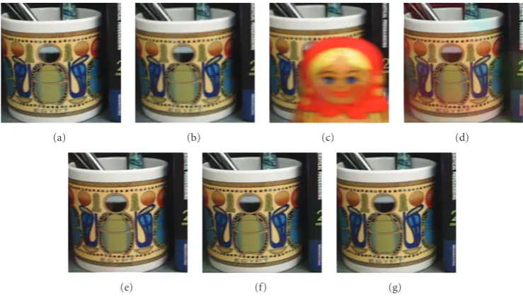
Figure4: 2×superresolution reconstruction results for the12-frames Egyptian Mug sequence:(a) original HR frame #1 (ground truth), (b) LR frame #1, (c) LR frame #5, (d) SR estimate usingL2error norm + Tikhonov regularization. (e) SR estimate usingL1error norm + Tikhonov
regularization, (f) SR estimate using the proposed algorithm without regularization, and (g) with Tikhonov regularization.
It is worth mentioning that although a number of superreso-lution reconstruction algorithms that incorporate color reg-ularization tying the color bands have been introduced in the literature [29–31,34], in this paper, however, we have not in-cluded any such regularization terms in the objective func-tion because this will obscure the impact of the influence function of a given M-estimator. Also, the goal is to empha-size the effect of the influence function on the reconstruction process.
In this section, experiments with both synthetic and real sequences are demonstrated, and the notationr× superreso-lution is used to denote increasing the resosuperreso-lution of the first (reference) frame in a given sequence by a factor ofrin each of thexandydirections.
4.1. 4×SR experiment: the SMU Helmet sequence
In this experiment, a sequence of 16 LR frames is syntheti-cally generated from an HR image (the SMU Helmet image shown inFigure 2(a)) as follows. A set of 16 integer shift pairs (in both thexandydirections) is generated and the HR im-age is shifted by these shift values. Frames #4 and #10 are rotated and zoomed in, respectively, to create general affine motion. The resulting 16 warped frames are then convolved with a normalized 5×5 Gaussian kernel of zero mean and variance of 0.5, and downsampled by a factor of 4 in both thexandydirections. The MATLAB functionfspecialis used to generate the Gaussian kernel. A zero-mean Gaussian noise is then added to the resulting LR frames such that each has a signal-to-noise ratio of 25 dB. The MATLAB function im-noiseis used to add the Gaussian noise. It is worth mention-ing that warpmention-ing, blurrmention-ing, downsamplmention-ing, and noise addi-tion are performed on each of the color components (R,G, andB) of the HR image separately. To simulate motion
es-timation errors, a translational motion model is assumed. In addition, a motion bias of 4 pixels (in the HR grid) is added to the motion vector of frame #13 (to each of its three color components). To simulate blur estimation errors, the PSF is assumed to be a normalized 5×5 Gaussian kernel of zero mean and unity variance. Figures2(b)and2(c)show LR frames #1 and #4, respectively.
The SR estimate using theL2error norm and Tikhonov
regularization is shown inFigure 2(d).βandλwere both set to 0.1. From this result, it is shown that theL2estimate suffers
from noticeable artifacts due to the outliers (the shadows cor-responding to the rotated and zoomed frames appear clearly in the background). This result is not surprising, since theL2
error norm is vulnerable to the outliers because of its linear influence function that assigns larger weights to larger errors, and hence amplifies their influence in the estimation. The SR estimate using theL1error norm and Tikhonov
regulariza-tion is shown inFigure 2(e).βandλwere set to 2 and 0.02, respectively. From this result, it is shown how using theL1
er-ror norm has suppressed the outliers compared to using the L2 error norm. However, as discussed inSection 2, because
of its constant valued influence function (±1), it results in a blurry SR estimate of a relatively poor quality.
The SR reconstruction result using the proposed scheme without regularization is shown in Figure 2(h). From this result, it is observed how the proposed approach has suc-cessfully suppressed the effect of the outliers, resulting in artifacts-free SR estimate of crisp details.Figure 2(i)depicts the SR estimate using the proposed scheme with Tikhonov regularization (λ = 0.2). The use of regularization slightly improved the visual appearance of the SR estimate because of the imposed smoothness constraint.
Figure 3depicts plots of the average SAD (dk’s), the
12 10 8 6 4 2
k(frame index) 0
20 40 60 80
dk
Red component Green component Blue component
(a)
12 10 8 6 4 2
k(frame index) 0
50 100 150 200
τk
Red component Green component Blue component
(b)
200 100 0 −100 −200
er −1
−0.5 0 0.5 1
ψk
(
er
)
(c)
200 100 0 −100 −200
eg −1
−0.5 0 0.5 1
ψk
(
eg
)
(d)
200 100 0 −100 −200
eb −1
−0.5 0 0.5 1
ψk
(
eb
)
(e)
Figure5:Superresolution reconstruction results of the12-frames Egyptian Mug sequence using the proposed approach: (a) plot of average SAD values (dk’s) for the three color components, (b) plot of the outlier thresholds (τk’s) for the three color components, and plot of the
Lorentzian influence functions (ψk’s) for the (c) red component, (d) green component, and (e) blue component. From (c) to (e), the red
curves correspond to LR frames #4, #5, and #6, where the matryoshka doll occludes big parts of the scene.
(ψk’s) for the 16 LR frames of the SMU Helmet sequence. In
Figures3(c)–3(e), the red, green, and magenta curves corre-spond to the LR frames #4, #10, and #13, respectively. From these plots, it is shown how the average SAD measure cap-tures the mismatch between the three outliers’ frames and the reference (first) LR frame. It is also noted that the outlier thresholds corresponding to frame #4 and #10 are consider-ably small because of their extreme violation of the assumed translational motion model. Whereas the outlier threshold
4.2. 2×SR experiment: the Egyptian Mug sequence
In this experiment, a sequence of 12 compressed frames (MJPEG) is captured by a handheld camera, CanonPower Shot A400. This sequence follows approximately the global translation motion. Occlusion is introduced by moving a matryoshka doll into the scene in 4 frames (4–7). The LR se-quence of frames is obtained from the original HR sese-quence captured by the camera via downsampling by a factor of 2 in both thexandydirections. Figures4(a)–4(c)show the origi-nal HR frame #1 (ground truth), LR frame #1, and LR frame #5 in which the matryoshka doll occludes the Egyptian-Mug, respectively. It is worth mentioning that occlusion was intro-duced intentionally in this sequence to simulate accidental scene changes that typically occur in real video sequences. A translational motion model is assumed, and the algorithm in [35] is used to estimate the motion vectors for each ofR,G, andBcomponents, separately. Theunknowncamera PSF is assumed to be a normalized 5×5 Gaussian kernel of zero mean and unity variance and the MATLAB functionfspecial is used to generate this kernel.
The SR estimate using theL2error norm and Tikhonov
regularization is shown in Figure 4(d).βandλwere set to 0.5, and 0.1, respectively. From this result, it is shown that the L2 estimate suffers from excessive false color artifacts.
These artifacts result from the matryoshka doll whose color is mostly yellow and red. The SR estimate using theL1error
norm and Tikhonov regularization is shown inFigure 4(e). βandλwere set to 2 and 0.025, respectively. From this result, it is shown how using theL1 error norm results in a better
estimate than that using theL2error norm. However, the SR
estimate also suffers from noticeable false (reddish) coloring. The SR reconstruction results using the proposed scheme without and with Tikhonov regularization (λ = 0.15) are shown in Figures4(f)and4(g), respectively. From these re-sults, it is observed how the proposed approach results in a SR estimate of crisp details and no color artifacts, even with-out the use of color regularization in the objective function.
Figure 5depicts plots of the average SAD (dk’s), the
out-lier thresholds (τk’s) and the Lorentzian influence functions
(ψk’s) for the 12 LR frames of the Egyptian-Mug sequence.
In Figures 5(c)–5(e), the red curves correspond to the LR frames #4–#6, in which the matryoshka doll occludes big po-tions of the scene. From these plots, it is shown how the av-erage SAD measure captures the mismatch between the out-liers’ frames, in which the matryoshka doll occludes the Mug, and the reference (first) LR frame. It is also noted that the outlier thresholds corresponding to outliers’ frames for the red component are considerably smaller than those for the green and blue components, and those for the green compo-nent are smaller than those for the blue compocompo-nent. This is because the colors of the matryoshka doll are mostly red and yellow. From these results, it is shown that computing differ-ent outlier thresholds for each of the three color compondiffer-ents is very effective in dealing with outliers that might appear in one (or more) color component and not in the rest of the color components.
5. SUMMARY
In this paper, a new adaptive M-estimation framework has been presented for robust color image super-resolution. Us-ing a robust error norm in the data fidelity term of the objec-tive function, and adapting the estimation process to each of the low-resolution frames and each of the color components, the proposed method effectively suppresses the outliers due to model violations, and results in color SR images of crisp details and no artifacts, without the use of regularization. Ex-perimental results on both synthetic and real sequences have demonstrated the superior performance of the proposed al-gorithm over using theL2and theL1error norms in the
ob-jective function. We are currently investigating the extension of the proposed solution to video sequences in which dealing with local outliers will be addressed.
APPENDIX
DERIVATION OF(18)
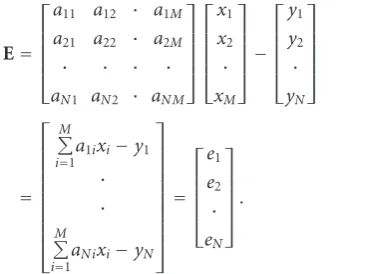
LetE =DHFX−Y =AX−Y, whereAisN×M. ThenE can be written as
E= ⎡ ⎢ ⎢ ⎢ ⎢ ⎣
a11 a12 · a1M
a21 a22 · a2M
· · · ·
aN1 aN2 · aNM
⎤ ⎥ ⎥ ⎥ ⎥ ⎦ ⎡ ⎢ ⎢ ⎢ ⎢ ⎣ x1 x2 · xM ⎤ ⎥ ⎥ ⎥ ⎥ ⎦− ⎡ ⎢ ⎢ ⎢ ⎢ ⎣ y1 y2 · yN ⎤ ⎥ ⎥ ⎥ ⎥ ⎦ = ⎡ ⎢ ⎢ ⎢ ⎢ ⎢ ⎢ ⎢ ⎢ ⎢ ⎣ M
i=1a1ixi−y1 · ·
M
i=1aNixi−yN ⎤ ⎥ ⎥ ⎥ ⎥ ⎥ ⎥ ⎥ ⎥ ⎥ ⎦ = ⎡ ⎢ ⎢ ⎢ ⎢ ⎣ e1 e2 · eN ⎤ ⎥ ⎥ ⎥ ⎥ ⎦. (A.1)
Sinceρ(E) is an error norm, it follows thatρ(E)=jρ(ej)
and the derivative ofρ(E) with respect toXis
∇ρ(E)=
∂ρ(E) ∂x1
∂ρ(E) ∂x2 · · ·
∂ρ(E) ∂xM
T
. (A.2)
Letψ(e) = ∂ρ(e)/∂e, applying chain rule and using (A.1), (A.2) can be written as
∇ρ(E)=
N
j=1aj1ψ
ej
· · · N
j=1ajMψ
ej
T
=ATψe
1
· · · ψeN
T
=⇒ ∇ρ(E)=ATψ(E)=(DHF)T
ψ.
(A.3)
Substituting by (A.3) in (17), we get
Xni+1=Xin−η L
k=1
∇ρEni,k;τi,k
=Xin−η L
k=1
DHFi,k
T
ψn
i,k, n=0, 1, 2,. . ., i=R,G,B.
ACKNOWLEDGMENT
This research was supported in part by the US ARL Grant no. W911NF-06-2-0035.
REFERENCES
[1] P. J. Huber,Robust Statistics, Wiley Series in Probability and Statistics, John Wiley & Sons, New York, NY, USA, 2003. [2] F. R. Hampel, E. M. Ronchetti, P. J. Rousseeuw, and W. A.
Sta-hel,Robust Statistics: The Approach Based on Influence Func-tions, Wiley Series in Probability and Statistics, John Wiley & Sons, New York, NY, USA, 2005.
[3] R. A. Maronna, D. R. Martin, and V. J. Yohai,Robust Statistics: Theory and Methods, Wiley Series in Probability and Statistics, John Wiley & Sons, New York, NY, USA, 2006.
[4] N. Sebe and M. S. Lew,Robust Computer Vision: Theory and Applications, Springer, Berlin, Germany, 2003.
[5] M. J. Black and P. Anandan, “The robust estimation of mul-tiple motions: parametric and piecewise-smooth flow fields,”
Computer Vision and Image Understanding, vol. 63, no. 1, pp. 75–104, 1996.
[6] T. Rabie, “Robust estimation approach for blind denoising,”
IEEE Transactions on Image Processing, vol. 14, no. 11, pp. 1755–1765, 2005.
[7] M. J. Black, G. Sapiro, D. H. Marimont, and D. Heeger, “Ro-bust anisotropic diffusion,”IEEE Transactions on Image Pro-cessing, vol. 7, no. 3, pp. 421–432, 1998.
[8] P. Meer, D. Mintz, A. Rosenfeld, and D. Y. Kim, “Robust re-gression methods for computer vision: a review,”International Journal of Computer Vision, vol. 6, no. 1, pp. 59–70, 1991. [9] D. Capel, Image Mosaicing and Superresolution, Springer,
Berlin, Germany, 2004.
[10] N. A. El-Yamany, P. E. Papamichalis, and W. R. Schucany, “A robust image superresolution scheme based on redescending M-estimators and information-theoretic divergence,” in Pro-ceedings of IEEE International Conference on Acoustics, Speech and Signal Processing (ICASSP ’07), vol. 1, pp. 741–744, Hon-olulu, Hawaii, USA, April 2007.
[11] V. Patanavijit and S. Jitapunkul, “A Lorentzian stochas-tic estimation for a robust iterative multiframe superreso-lution reconstruction with Lorentzian-Tikhonov regulariza-tion,” EURASIP Journal on Advances in Signal Processing, vol. 2007, Article ID 34821, 21 pages, 2007.
[12] V. Patanavijit, S. Tae-O-Sot, and S. Jitapunkul, “A robust iter-ative superresolution reconstruction of image sequences using a Lorentzian Bayesian approach with fast affine block-based registration,” inProceedings of IEEE International Conference on Image Processing (ICIP ’07), vol. 5, pp. 393–396, San Anto-nio, Tex, USA, September-October 2007.
[13] N. A. El-Yamany and P. E. Papamichalis, “An adaptive M-estimation framework for robust image superresolution with-out regularization,” inVisual Communications and Image Pro-cessing, vol. 6822 ofProceedings of SPIE, pp. 1–12, San Jose, Calif, USA, January 2008.
[14] S. C. Park, M. K. Park, and M. G. Kang, “Superresolution im-age reconstruction: a technical overview,”IEEE Signal Process-ing Magazine, vol. 20, no. 3, pp. 21–36, 2003.
[15] M. Elad and A. Feuer, “Restoration of a single superresolution image from several blurred, noisy, and undersampled mea-sured images,”IEEE Transactions on Image Processing, vol. 6, no. 12, pp. 1646–1658, 1997.
[16] M. Elad and Y. Hel-Or, “A fast superresolution reconstruction algorithm for pure translational motion and common space-invariant blur,”IEEE Transactions on Image Processing, vol. 10, no. 8, pp. 1187–1193, 2001.
[17] A. Zomet and S. Peleg, “Efficient superresolution and applica-tions to mosaics,” inProceedings of the 15th International Con-ference on Pattern Recognition (ICPR ’00), vol. 1, pp. 579–583, Barcelona, Spain, September 2000.
[18] A. Zomet, A. Rav-Acha, and S. Peleg, “Robust superresolu-tion,” inProceedings of IEEE Computer Society Conference on Computer Vision and Pattern Recognition (CVPR ’01), vol. 1, pp. 645–650, Kauai, Hawaii, USA, December 2001.
[19] N. Nguyen, P. Milanfar, and G. Golub, “A computationally ef-ficient superresolution image reconstruction algorithm,”IEEE Transactions on Image Processing, vol. 10, no. 4, pp. 573–583, 2001.
[20] S. Farsiu, D. Robinson, M. Elad, and P. Milanfar, “Robust shift and add approach to superresolution,” inApplications of Digi-tal Image Processing XXVI, vol. 5203 ofProceedings of SPIE, pp. 121–130, San Diego, Calif, USA, August 2003.
[21] S. Farsiu, M. D. Robinson, M. Elad, and P. Milanfar, “Fast and robust multiframe superresolution,”IEEE Transactions on Im-age Processing, vol. 13, no. 10, pp. 1327–1344, 2004.
[22] S. Farsiu, D. Robinson, M. Elad, and P. Milanfar, “Advances and challenges in superresolution,” International Journal of Imaging Systems and Technology, vol. 14, no. 2, pp. 47–57, 2004.
[23] E. S. Lee and M. G. Kang, “Regularized adaptive high-resolution image reconstruction considering inaccurate sub-pixel registration,” IEEE Transactions on Image Processing, vol. 12, no. 7, pp. 826–837, 2003.
[24] M. C. W. Zibetti and J. Mayer, “Outlier robust and edge-preserving simultaneous superresolution,” in Proceedings of IEEE International Conference on Image Processing, pp. 1741– 1744, Atlanta, Ga, USA, October 2006.
[25] M. Trimeche, R. C. Bilcu, and J. Yrj¨an¨ainen, “Adaptive outlier rejection in image superresolution,”EURASIP Journal on Ap-plied Signal Processing, vol. 2006, Article ID 38052, 12 pages, 2006.
[26] W.-Y. Zhao and H. S. Sawhney, “Is superresolution with opti-cal flow feasible?” inProceedings of the 7th European Conference on Computer Vision-Part I (ECCV ’02), vol. 2350 ofLecture Notes in Computer Science, pp. 599–613, Copenhagen, Den-mark, May 2002.
[27] Z. A. Ivanovski, L. Panovski, and L. J. Karam, “Robust super-resolution based on pixel-level selectivity,” inVisual Commu-nications and Image Processing, vol. 6077 ofProceedings of SPIE, pp. 1–8, San Jose, Calif, USA, January 2006.
[28] C. A. Segall, A. K. Katsaggelos, R. Molina, and J. Mateos, “Superresolution from compressed video,” inSuperresolution Imaging, S. Chaudhuri, Ed., pp. 211–242, chapter 9, Kluwer Academic Publishers, Dordrecht, The Netherlands, 2001. [29] S. Farsiu, M. Elad, and P. Milanfar, “Multiframe
demosaic-ing and superresolution of color images,”IEEE Transactions on Image Processing, vol. 15, no. 1, pp. 141–159, 2006. [30] S. Farsiu, M. Elad, and P. Milanfar, “Video-to-video
dy-namic superresolution for grayscale and color sequences,”
EURASIP Journal on Applied Signal Processing, vol. 2006, Ar-ticle ID 61859, 15 pages, 2006.
[31] B. C. Tom and A. K. Katsaggelos, “Resolution enhancement of monochrome and color video using motion compensation,”
[32] D. P. Bertsekas, Nonlinear Programming, Athena Scientific, Belmont, Mass, USA, 1999.
[33] A. Blake and A. Zisserman,Visual Reconstruction, MIT Press, Cambridge, Mass, USA, 1987.
[34] N. R. Shah and A. Zakhor, “Resolution enhancement of color video sequences,”IEEE Transactions on Image Processing, vol. 8, no. 6, pp. 879–885, 1999.