A Patch-Based Structural Masking Model with an Application to Compression

(1)

doi:10.1155/2009/649316

Research Article

A Patch-Based Structural Masking Model with

an Application to Compression

Damon M. Chandler,

1

_{Matthew D. Gaubatz,}

2

_{and Sheila S. Hemami}

3 1_{School of Electrical and Computer Engineering, Oklahoma State University, Stillwater, OK 74078, USA} 2_{Print Production Automation Lab, HP Labs, Hewlett-Packard, Palo Alto, CA 94304, USA}

3_{School of Electrical and Computer Engineering, Cornell University, Ithaca, NY 14853, USA}

Correspondence should be addressed to Matthew D. Gaubatz,[email protected]

Received 26 May 2008; Accepted 25 December 2008

Recommended by Simon Lucey

The ability of an image region to hide ormaska given target signal continues to play a key role in the design of numerous image

processing and vision systems. However, current state-of-the-art models of visual masking have been optimized for artificial targets placed upon unnatural backgrounds. In this paper, we (1) measure the ability of natural-image patches in masking distortion; (2) analyze the performance of a widely accepted standard masking model in predicting these data; and (3) report optimal model

parameters for diﬀerent patch types (textures, structures, and edges). Our results reveal that the standard model of masking

does not generalize across image type; rather, a proper model should be coupled with a classification scheme which can adapt the model parameters based on the type of content contained in local image patches. The utility of this adaptive approach is demonstrated via a spatially adaptive compression algorithm which employs patch-based classification. Despite the addition of

extra side information and the high degree of spatial adaptivity, this approach yields an eﬃcient wavelet compression strategy that

can be combined with very accurate rate-control procedures.

Copyright © 2009 Damon M. Chandler et al. This is an open access article distributed under the Creative Commons Attribution License, which permits unrestricted use, distribution, and reproduction in any medium, provided the original work is properly cited.

1. Introduction

Visual masking is a general term that refers to the perceptual phenomenon in which the presence of a masking signal (the mask) reduces a subject’s ability to visually detect another signal (the target of detection). Masking is perhaps the single most commonly used property of the human visual system for image processing. It has found extensive use in image and video compression [1–4], digital watermarking [5–9], unequal error protection [10], quality assessment [11– 14], image synthesis [15,16], in the design of printers and variable-resolution displays [17, 18], and in several other areas (e.g., in image denoising [19] and camera projection [20]). For most of these applications, the original image serves as the mask, and the distortions induced via the processing (e.g., compression artifacts, rendering artifacts, or a watermark) or specific objects of interest (e.g., in object tracking) serve as the target of detection. Predicting an image’s ability to mask a visual target is thus of great interest to system designers.

The amount of masking imposed by a particular image is determined by measuring a human subject’s ability to detect a target in the presence of the mask. A psychophysical experiment of this type would commonly employ a forced-choice procedure in which two images are presented to a subject. One image contains just the mask (e.g., an original image patch), and the other image contains the mask+target (e.g., a distorted image patch). The subject is then asked to select which of the two images contains the target. If the subject chooses the correct image, the contrast of the target is reduced; otherwise, the contrast of the target is increased. This process is repeated until the contrast of the target is at the subject’s threshold of detectability.

(2)

commonly modeled via three stages: (1) a frequency-based decomposition which models the initially linear responses of an array of visual neurons, (2) application of a pointwise nonlinearity to the transform coefficients and inhibition based on the values of other coefficients (gain control [24– 27]), and (3) summation of these adjusted coefficients across space, spatial frequency, and orientation so as to arrive at a single scalar response value for each image. The first two stages, in effect, represent the two images (mask and mask+target) as points in a feature space, and the target is deemed visually detectable if the two points are sufficiently distant (as measured, in part, in the third stage).

Standard approaches to the frequency-based decomposi-tion include a steerable pyramid [22], a Gaussian pyramid [11], an overcomplete wavelet decomposition [28], radial filters [29], and cortex filters [21, 24, 30]. The standard approach to the summation stage employs a p-norm, typically with p ∈ [1.5, 4]. The area of greatest debate lies in the implementation of the second stage which models the pointwise nonlinearity and the gain control mechanism provided by the inhibitory pool [24,27,31]. Letx(u0,f0,θ0) correspond to the transform coeﬃcient at locationu0, center frequency f0, and orientationθ0. In a standard gain-control-based masking model, the (nonlinear) response of a neuron tuned to these parameters,r(u0,f0,θ0), is given by

ru0,f0,θ0

=g·

wf0,θ0

xu0,f0,θ0 p

bq₊ (u,f,θ)∈S

w(f,θ)x(u,f,θ)q, (1)

where g is a gain factor, w(f,θ) represents a weight designed to take into account the human contrast sensitivity function, b represents a saturation constant, p provides the pointwise nonlinearity to the neuron, q provides the pointwise nonlinearity to the neurons in the inhibitory pool, and the setSindicates which other neurons are included in the inhibitory pool.

Although numerous studies have shown that the response of a neuron can be attenuated based on the responses of neighboring neurons (see, e.g., [26, 32]), the actual contributors to the inhibitory pool remain largely unknown. Accordingly, the specific parameters used in gain-control-based masking models are generally fit to experi-mental masking data. For example, model parameters have been optimized for detection thresholds measured using simple sinusoidal gratings [4], to filtered white noise [3], and to threshold-versus-contrast (TvC) curves of target Gabor patterns with sinusoidal maskers [22,24]. Typically, p and q are in the range 2 ≤ q ≤ p ≤ 4, and the inhibitory pool consists of neural responses in the same spatial frequency band (f0), at orientations within ±45◦ of θ0, and within a local spatial neighborhood (e.g., 8-connected neighbors). Indeed, this approach has proved quite successful at predicting detection thresholds for targets placed against relatively simplistic masks such as sinusoidal gratings, Gabor patches, or white noise.

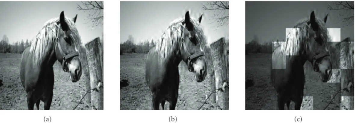
Image-processing applications however, are concerned with the detectability of specific targets presented against naturalistic, structured backgrounds rather than white noise or other artificial masks. It remains an open question of whether the model parameters need to be adjusted for masks consisting of natural images, and if so, what are the proper adjustments? Because very few studies have measured masking data for natural-image stimuli [33–35], the optimal model parameters for natural-image masks have yet to be determined. Consequently, the majority of current algo-rithms simply use the aforementioned standard parameter values (optimized for simplistic masks). Although we have previously shown that the use of these standard model parameters can provide reasonable predictions of masking imposed by textures [6], most natural images contain a mix oftextures, structures, andedges. We have observed that application of these standard model parameters to natural images often leads to overestimates of the ability of edges and object boundaries to mask distortions. This shortcoming is illustrated in Figure 1, which depicts an original image of a horse (a), that same image to which wavelet subband quantization distortions oriented at 90◦ have been been added (b), and the top ten 32×32 patches which contain the most visible distortions (c) as estimated by a standard model of masking ((1) with p = 2.4, q = 2.3, b =

0.03, and g = 0.025; see Section 3 for further details of the model implementation). Notice from the middle image of Figure 1that the distortions are most visible in the flat regions of sky around the horse’s ears. Yet, the masking model overestimates the ability of these structured regions to mask the distortion.

To address this issue, the goals of this paper are threefold. (1) We present the results of a psychophysical experiment which provides masking data using natural-image patches; our results confirm the fact that edges and other structured regions provide less masking than textures. (2) Based on these masking data, we present model parameters which are optimized for natural image content (textures, structures, and edges) and are thus better suited for applications which process natural images. (3) We demonstrate the utility of this model for image processing via a specific application to image compression; a classification-based compression strategy is presented in which quantization step sizes are selected on a patch-by-patch basis as a function of the patch classification into a texture, structure, or edge, and then based upon our masking data. Despite the requirement of additional side information, the use of our image-type-specific masking data results in an average rate savings of 8%, and produces images that are preferred by 2/3 of tested viewers over a standard gain-control-based compression scheme.

(3)

(a) (b) (c)

Figure1: (a) Original 256×256 imagehorse. (b) Distorted version ofhorsecontaining wavelet subband quantization distortions created

via the following: (1) performing a three-level discrete wavelet transform of the original image using the 9/7 biorthogonal filters [36]; (2)

quantizing the HL subband at the third decomposition level with a step size of 400; (3) performing an inverse discrete wavelet transform. (c)

Highlighted regions correspond to the top ten 32×32 patches containing the most visible distortions as deemed by the standard masking

model; these blocks elicit the greatest diﬀerence in simulated neural responses between the original and distorted images (seeSection 3for

details of the model implementation). Notice from (b) that the distortions are most visible in the regions above the horse’s ears, whereas the masking model overestimates the ability of these regions in masking the distortion.

2. Visual Masking Experiment

In this work, atextureis defined as image content for which threshold elevation is reasonably well predicted by current masking models, and roughly matches our intuitive idea of what the term “texture” represents. An edge is one or more boundaries between homogeneous regions. Astructure is neither an edge nor a texture, but which contains some recognizable organization.

To investigate the eﬀects of patch contrast and type (texture, structure, edge) on the visibility of wavelet sub-band quantization distortions, a psychophysical detection experiment was performed. Various patches cropped from a variety of natural images served as backgrounds (masks) in this study. The patches were selected to contain either a texture, a structure, or an edge. We then measured the minimum contrast required for subjects to detect vertically oriented wavelet subband quantization distortions (targets) as a function of both the RMS contrast of each patch and the patch type.

We acknowledge that this division into three classes is somewhat restrictive and manufactured. Our motivation for using three categories stems primarily from our experience in applying masking models to image processing applications (compression [37–39], watermarking [6], and image and video quality assessment [13, 40]). We have consistently observed that the standard model of masking performs well on textures, but this same model always overestimates the masking ability of edges and other object boundaries. Thus, a logical first step toward extending the standard model of masking is to further investigate these two particular image types both psychophysically and computationally.

In addition, we have employed a third class, structures, to encompass regions which would not normally be considered an edge nor a texture. From a visual complexity standpoint, these are regions which are not as simple as an edge, but which are also less random (more structurally organized)

than a texture. We acknowledge that the structure class is broader than the other two classes, and that the term “structure” might not be the ideal label for all nonedge and nontexture patches. However, our motivation for using this additional class stems again from masking. For visual detection, we would expect structures to provide more masking than edges, but less masking than textures; thus, the structure class is a reasonable third choice to investigate. As discussed in this section, our psychophysical results confirm this rank ordering of masking ability. Furthermore, as we demonstrate inSection 4, improvements in visual quality can be achieved by modifying the standard model to take into account these three patch classes.

2.1. Methods

2.1.1. Apparatus and Contrast Metric. Stimuli were displayed on a high-resolution, Dell UltraScan P991 19-inch monitor at a display resolution of 28 pixels/cm. The display yielded minimum and maximum luminances of, respectively, 1.2 and 99.2 cd/m2, and an overall gamma of 2.3. Luminance measurements were made by using a Minolta LS-100 pho-tometer (Minolta Corporation, Tokyo, Japan). The pixel-value-to-luminance response of this monitor was approxi-mated via

L(X)=(0.7 + 0.026X)2.3, (2)

whereLdenotes the luminance in cd/m2, andXdenotes the 8 bit digital pixel value in the range 0–255. Stimuli were viewed binocularly through natural pupils in a darkened room at a distance of approximately 82 cm, resulting in a display visual resolution of 36.8 pixels/degree of visual angle [41].

(4)

contrast has been applied to a variety of stimuli, including noise [42], wavelets [43], and natural images [35,44]. In this paper, results are reported in terms of the RMS contrast of the distortions (target) computed with respect to the mean luminance of the background-image patch (mask). LetIand Idenote an original and distorted image patch, respectively, and, let E = I−I + (1/N)N_i=1Ii denote the mean-oﬀset distortions. The RMS contrast of the distortions,C, is given by

C= 1

μL(I)

1 N

N

i=1

LEi

−μL(E) 2 1/2

, (3)

whereμL(I)=(1/N) N

i=1L

Ii) denotes the average luminance of I, andN denotes the number of pixels in I, and where μL(E) = (1/N)

N i=1L

Ei) denotes the average luminance of the mean-oﬀset distortionsE. The quantitiesLIi) andL

Ei) correspond to the luminance of theith pixel of the image patch and the mean-oﬀset distortions, respectively.

2.1.2. Stimuli. Stimuli used in this study consisted of image patches containing wavelet subband quantization distor-tions. Each stimulus was composed of a mask upon which a target was placed. The masks were 64×64-pixel image patches. The targets were wavelet subband quantization distortions.

Masks. The masks used in this study consisted of 64× 64-pixel patches cropped from 8 bit grayscale images chosen from a database of high-resolution natural images. Fourteen 64 × 64 masks were used, four of which were visually categorized as containing primarily texture, five of which were visually categorized as containing primarily structure, and five of which were visually categorized as containing primarily edges. Figure 2depicts each mask along with its assigned common image name.

To investigate the eﬀect of mask contrast on target detectability, the RMS contrast of each mask was adjusted via

I=αI−μI

+μI, (4)

where I and I denote the original and contrast-adjusted images, respectively, where μI = (1/N)

N

i=1Ii denotes the mean pixel value of I, and where the scaling factor αwas chosen via bisection such that I was at the desired RMS contrast. (The RMS contrast of each mask was computed by using (3) with LIi) and μL(I) in place of, resp., L

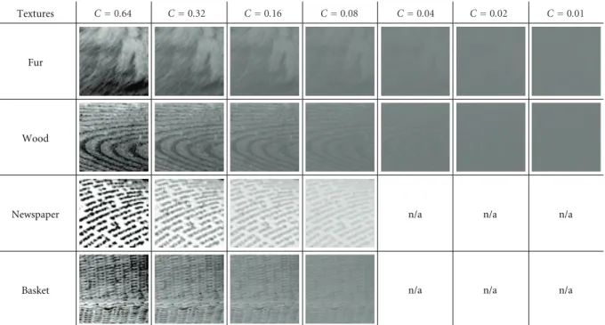
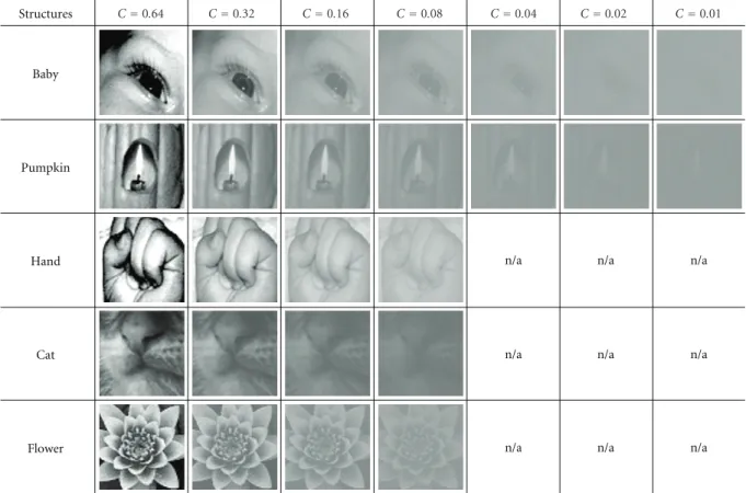
Ei) andμL(E).) RMS contrasts of 0.08, 0.16, 0.032, and 0.64 were used for all masks. To test the low-mask-contrast regime, two masks from each category were further adjusted to RMS contrasts of 0.01, 0.02, and 0.04 (imagesfurandwoodfrom the texture category, images baby and pumpkin from the structure category, and images butterfly and sail from the edges category). Figures 3, 4, and 5 depict the adjusted-contrast textures, structures, and edges, respectively.

Targets. The visual targets consisted of distortions generated via quantization of a single wavelet subband. The subbands

were obtained by applying a discrete wavelet transform (DWT) to each 64×64 patch using three decomposition levels and the 9/7 biorthogonal DWT filters (also used by Watson et al. [41], and by Ramos and Hemami [45], see also [35]). The distortions were generated via uniform scalar quantization of the HL3 subband (the subband at the third level of decomposition corresponding to vertically oriented wavelets). The quantizer step size was selected such that the RMS contrast of the resulting distortions was as requested by the adaptive staircase procedure (described in the following section). At the display visual resolution of 36.8 pixels/degree, the distortions corresponded to a center spatial frequency of 4.6 cycles/degree of visual angle.

Figures 6, 7, and 8 depict the masks from each cate-gory (texture, structure, and edge, resp.) along with each mask+target (distorted image). All masks in these figures have an RMS contrast of 0.32. All targets (distortions) are at an RMS contrast of 0.1. For illustrative purposes, the bottom row of each figure depicts just the targets placed upon a solid gray background set to the mean pixel value of each corresponding mask (i.e., the image patch has been replaced with its mean pixel value to facilitate viewing of just the distortions).

2.1.3. Procedures. Contrast thresholds for detecting the tar-get (distortions) in the presence of each mask (patch) were measured by using a spatial two-alternative forced-choice procedure. On each trial, observers concurrently viewed two adjacent images placed upon a solid gray 25 cd/m2 background. One of the images contained the mask alone (nondistorted patch) and the other image contained the mask+target (distorted image patch). The image to which the target was added was randomly selected at the beginning of each trial. Observers indicated via keyboard input which of the two images contained the target. If the choice was incorrect (target undetectable), the contrast of the target was increased; if the choice was correct (target detectable), the contrast of the target was decreased. This process was repeated for 48 trials, whereupon the final target contrast was recorded as the subject’s threshold of detection.

Contrast threshold was defined as the 75% correct point on a Weibull function, which was fitted to the data following each series of trials. Target contrasts were controlled via a QUEST staircase procedure [46] using software derived from the Psychophysics Toolbox [47,48]. During each trial, an auditory tone indicated stimulus onset, and auditory feedback was provided upon an incorrect response. Response time was limited to within 7 seconds of stimulus onset.

(5)

Textures:

Fur Wood Newspaper Basket

Structures:

Baby Pumpkin Hand Cat Flower

Edges:

Butterfly Sail Post Handle Leaf

Figure2: Image patches used as masks in the experiment. Textures:fur, wood, newspaper, and basket; structures:baby, pumpkin, hand, cat, and flower; edges:butterfly, sail, post, handle, and leaf.

Textures

Fur

Wood

Newspaper

Basket

n/a n/a

n/a

n/a n/a

n/a

C=0.64 C=0.32 C=0.16 C=0.08 C=0.04 C=0.02 C=0.01

Figure3: Contrast-adjusted versions of the textures used in the experiment. Note that only two images were tested in the very-low-contrast regime (RMS contrasts of 0.01, 0.02, and 0.04).

2.1.4. Subjects. Four adult subjects (including one of the authors) participated in the experiment. Three of the subjects were familiar with the purpose of the experiment; one of the subjects was naive to the purpose of the experiment. Subjects ranged in age from 20 to 30 years. All subjects had either normal or corrected-to-normal visual acuity.

2.2. Masking Results and Analysis

(6)

Structures

Baby

Pumpkin

Hand

Cat

Flower

n/a n/a

n/a

n/a n/a

n/a

n/a n/a

n/a

C=0.64 C=0.32 C=0.16 C=0.08 C=0.04 C=0.02 C=0.01

Figure4: Contrast-adjusted versions of the structures used in the experiment. Note that only two images were tested in the very-low-contrast regime (RMS contrasts of 0.01, 0.02, and 0.04).

the contrast of the mask. Figure 9(a) depicts the average results for textures along with individual TvC curves for imagesfurandwood.Figure 9(b)depicts the average results for structures along with individual TvC curves for images baby and pumpkin.Figure 9(c) depicts the average results for edges along with individual TvC curves for imagessail andbutterfly. In each graph, the horizontal axis denotes the RMS contrast of the mask, and the vertical axis denotes the RMS contrast of the target. The dashed line in each graph corresponds to the average TvC curve computed for all masks of a given category (texture, structure, and edge). Data points in the individual TvC curves indicate contrast detection thresholds averaged over all subjects. Error bars denote standard deviations of the means over subjects (individual TvC curves) and over masks (average TvC curves).

As shown in Figure 9, for mask contrasts below 0.04, the thresholds for all three image types (edges, textures, and structures) are roughly the same. Average thresholds when the mask contrast was at the minimum contrast tested of 0.01 were as follows. The error measurement reported for each threshold (represented by a ± sign) denotes one standard deviation of the mean over the tested images.

(i) Textures: 0.0080±0.0002, (ii) Structures: 0.0082±0.0001, (iii) Edges: 0.0089±0.0028.

Notice that the average thresholds for textures and structures are within each other’s standard deviation as well within as the standard deviation of the average threshold for edges. These data therefore suggest that at very low mask contrasts, in the regime in which the mask is nearly undetectable and certainly visually unrecognizable, masking is perhaps due primarily to either noise masking or low-level gain-control mechanisms (e.g., inhibition amongst V1 simple cells) [24], and not due to higher-level visual processing.

As previous masking studies have shown, when the contrast of the mask increases, so does the contrast threshold for detecting a target placed upon that mask. Our results support this finding; in general, the greater the mask contrast, the greater the detection threshold. However, as shown inFigure 9, the TvC curves for the three categories demonstrate a marked divergence as the contrasts of the masks increase. Average thresholds when the mask contrast was 0.64 (the maximum contrast tested) were as follows.

(i) Textures: 0.1233±0.0384, (ii) Structures: 0.07459±0.0218, (iii) Edges: 0.0288±0.0120.

(7)

Edges

Butterfly

Sail

Post

Handle

Leaf

n/a n/a

n/a

n/a n/a

n/a

n/a n/a

n/a

C=0.64 C=0.32 C=0.16 C=0.08 C=0.04 C=0.02 C=0.01

Figure5: Contrast-adjusted versions of the edges used in the experiment. Note that only two images were tested in the very-low-contrast regime (RMS contrasts of 0.01, 0.02, and 0.04).

Textures Fur Wood Newspaper Basket

Mask

Mask+target

Target

(8)

Structures Baby Pumpkin Hand Cat Flower

Mask

Mask+target

Target

Figure7: Structure masks (original images) at an RMS contrast of 0.32. Masks+targets (distorted images) in which the distortions are at an RMS contrast of 0.1. Targets (distortions) shown against a gray background set to the mean pixel value of the corresponding mask (shown for illustrative purposes only).

Edges Butterfly Sail Post Handle Leaf

Mask

Mask+target

Target

Figure8: Edge masks (original images) from each category at an RMS contrast of 0.32. Masks+targets (distorted images) in which the distortions are at an RMS contrast of 0.1. Targets (distortions) shown against a gray background set to the mean pixel value of the corresponding mask (shown for illustrative purposes only).

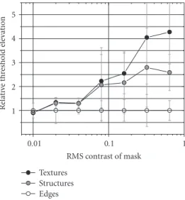
2.2.2. Detection Thresholds as a Function of Mask Category. The influence of patch content (mask category) on detection thresholds is further illustrated in Figures10and11, which depict relative threshold elevations defined as

relative threshold elevation= CT

CTedge

, (5)

where CT denotes the contrast detection threshold for a given mask contrast, and CTedge denotes the contrast detection threshold averaged over all edges of the same contrast. Thus, the relative threshold elevation provides a measure of the extent to which a given mask increases thresholds (for elevations >1.0) or decreases thresholds (elevations<1.0) relative to an edge of the same contrast. The

relative threshold elevation was computed separately for each subject and each mask.

(9)

0.01 0.1

RMS

co

nt

ra

st

of

target

0.01 0.1 1

RMS contrast of mask Fur

Wood Avg. all textures

(a)

0.01 0.1

RMS

co

nt

ra

st

of

target

0.01 0.1 1

RMS contrast of mask Baby

Pumpkin Avg. all structures

(b)

0.01 0.1

RMS

co

nt

ra

st

of

target

0.01 0.1 1

RMS contrast of mask Butterfly

Sail Avg. all edges

(c)

Figure9: Threshold-versus-contrast (TvC) curves obtained from the masking experiment. (a) Average TvC curve for textures (dashed line)

and individual TvC curves forfurandwood. (b) Average TvC curve for structures and individual TvC curves forbabyandpumpkin. (c)

Average TvC curves for edges and individual TvC curves forbutterflyandsail. In each graph, the horizontal and vertical axes correspond to

the RMS contrast of the mask (image) and the RMS contrast of the target (distortion), respectively. Data points in the individual TvC curves indicate contrast detection thresholds averaged over all subjects. Error bars denote standard deviations of the means.

1 2 3 4 5

R

elati

ve

thr

eshold

ele

vation

0.01 0.1 1

RMS contrast of mask Textures

Structures Edges

Figure 10: Average relative threshold elevations for each mask category plotted against mask contrast. For increasingly greater mask contrasts, textures and structures demonstrate increasingly greater threshold elevations over edges at the same contrast.

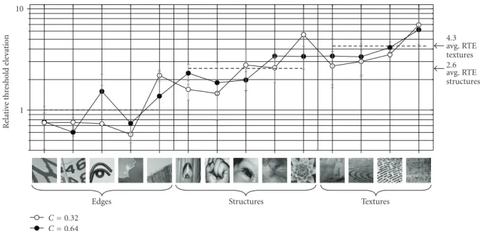
Figure 11 depicts relative threshold elevations for the 0.32 and 0.64 contrast conditions plotted for each of the 14 images. The data points denote relative threshold elevations averaged over all subjects; error bars denote standard deviations of the means over subjects. The dashed lines denote average relative threshold elevations for each of the three image types. The images depicted on the horizontal axis have been ordered by eye to represent a general transition from simplistic edge to complex texture (from left to right). Indeed, notice that the data generally demonstrate a corresponding left-to-right increase in relative threshold elevation.

Thus, on average, high-contrast (0.32–0.64) textures elevate detection thresholds approximately 4.3 times greater than high-contrast edges, and high-contrast structures ele-vate thresholds approximately 2.6 times greater than high-contrast edges. We call this eﬀectstructural masking which attributes elevations in threshold to the structural content (texture, structure, and edge) of the mask. (We are currently investigating the relationship between structural masking

and entropy masking [49]. Entropy masking attributes

elevations in thresholds to a subject’s unfamiliarity with a mask. A computational model of entropy masking has yet to be developed.) These findings demonstrate that a proper measure of masking should account both for mask contrast and for masktype. In the following section, we use these masking data to compute optimal mask-type-specific parameters for use in a gain-control-based masking model.

3. Fitting a Gain-Control Model to

Natural Images

The standard gain-control model, which has served as a cor-nerstone in current understanding of the nonlinear response properties of early visual neurons, has proved quite successful at predicting thresholds for detecting targets placed against relatively simplistic masks. However, gain-control models do not explicitly account for image content; rather, they employ a relatively oblivious inhibitory pool which imposes largely the same inhibition regardless of whether the mask is a texture, structure, or edge. Such a strategy is feasible for low-contrast masks, but, as demonstrated by our experimental results, high-contrast textures, structures, and edges impose significantly diﬀerent elevations in thresholds (i.e., structural masking is observed).

(10)

1 10

R

elati

ve

thr

eshold

ele

vation

Edges Structures Textures

4.3 avg. RTE textures 2.6 avg. RTE structures

C=0.32

C=0.64

Figure11: Relative threshold elevations averaged over all subjects for each of the 14 masks at contrasts of 0.32 and 0.64.

report the optimal model parameters. We demonstrate that when the model is implemented with standard parameter values, the model can perform well in predicting thresholds for textures. However, these same parameters lead to over-estimates of the amount of masking provided by edges and structures. Here, we report optimal model parameters for diﬀerent patch types (textures, structures, and edges) which provide a better fit to the masking data than that achieved by using standard parameter values.

3.1. A Discussion of Gain Control Models. The standard

model of gain control described inSection 1contains many parameters that must be set. However, we emphasize that this model is used extensively in the visual neuroscience community to mimic an underlying physical model consist-ing of an array of visual neurons. This neurophysiological underpinning limits the choice of model parameters to those which are biologically plausible. Here, before discussing the details of our model implementation, we provide general details regarding the selection of these parameters. For convenience, we repeat (1) as follows:

ru0,f0,θ0

=g·

wf0,θ0

xu0,f0,θ0 p

bq₊ (u,f,θ)∈S

w(f,θ)x(u,f,θ)q. (6)

As mentioned previously, this gain-control equation models a nonlinear neural response, which is implemented via a ratio of responses designed to mimic neural inhibition observed in V1 (so-called divisive normalization). The numerator models the excitatory response of a single neuron, and the denominator models the inhibitory responses of the neurons which impose the normalization.

3.1.1. The Input Gain w(f,θ) and Output Gain g. The parameters w(f,θ) and g model the input and output gain of each neuron, respectively. The input gainw(f,θ) is

designed to account for the variation in neural sensitivity to diﬀerent spatial frequencies and orientations. These gains are typically chosen to match the human contrast sensitivity function derived based on detection thresholds measured for unmasked sine-wave gratings (e.g., [21]). Others have selected the gains to match unmasked detection thresholds for Gabor or wavelet targets, which are believed to better probe the sensitivities of visual neurons (e.g., [24]). We have followed this latter approach.

The output gaingcan be viewed as the sensitivity of the neuron following divisive normalization. This parameter is typically left as a free parameter that is adjusted to match TvC curves. We too have leftgas a free parameter.

3.1.2. The Excitatory and Inhibitory Exponents pandq, and the Semisaturation Constant b. The parameters p and q, when used with (1), are designed to account for the fact that visual neurons exhibit a nonlinear response to contrast. A neuron’s response increases with increasing stimulus contrast, but this response begins to level oﬀ at higher contrasts. In [22], p andq were fixed at the same value of p=q=2. (Indeed, in terms of biological plausibility, using the same value for pandqis logical.) However, as noted by Watson and Solomon [24], this setting of p = q leads to premature response saturation in the model. In both [24,26], this side eﬀect is avoided by selecting separate values for p andq, with the condition thatp > qto prevent an eventual decrease in response at high contrast. Typically, pandqare in the range 2≤q≤p≤4. Most often, eitherporqis fixed, and other is left as a free parameter. We have followed this latter approach (pfixed,qfree).

(11)

fixed andbfree, each of which leads to an optimal value near 0.03 which is well within the range reported in [24].

3.2. Model Implementation. As mentioned in Section 1,

computational models of gain control typically employ three stages: (1) a frequency-based decomposition which models the initially linear responses of an array of visual neurons, (2) computation of nonlinear neural responses and inhibition, and (3) summation of modeled neural responses. The individual neural responses were modeled by using (1) with specific details of the model as described in what follows.

The initially linear responses of the neurons (x(f,u,θ) in (1)) were modeled by using a steerable pyramid decom-position with four orientations, 0◦, 45◦, 90◦, and 135◦, and three levels of decomposition performed on the original and distorted images. This decomposition was applied to the luminance values of each image computed via (2). The CSF weightsw(f,θ) were set to values of 0.068, 0.266, and 0.631 for bands from the first through third decomposition levels, respectively, and the same weights were used for all four orientations. These CSF weights were selected based on our previous study utilizing wavelet subband quantization distortions presented against a gray background (i.e., in the absence of a mask) [35].

The inhibitory pool consisted of those neural responses at orientations within ±45◦ of the orientation of the responding neuron and within the same frequency band as the responding neuron. Following from [13] (see also [24]), a Gaussian-weighted summation over space, implemented via convolution, was used for the inhibitory pool. Specifi-cally, the spatial extent of the inhibitory pooling was selected to be a 3×3 window (8 connected neighbors) in which the contribution of each neighbor was determined by the taps of a 3×3 Gaussian filter created via the outer product of one-dimensional filters with impulse response [1/6, 2/3, 1/6].

To determine if a target is at the threshold of detection, the modeled neural responses to the mask are compared with the modeled neural responses to the mask+target. Let{rmask(u,f,θ)}and{rmask+target(u,f,θ)}denote the sets of modeled neural responses computed via (1) for the mask and mask+target, respectively. The model deems the target detectable if{rmask(u,f,θ)}and{rmask+target(u,f,θ)} suﬃciently diﬀer as measured via

d=

u

θ

f

_r_mask₍_u_,_f_,_θ₎

−rmask+target(u,f,θ)βf

βθ/βfβu/βθ1/βu ,

(7)

withβθ =βf =1.5 andβu=2; the value ofβθ =βf =1.5 was selected based on our previous study on summation of responses to wavelet subband quantization distortions [35]. The model predicts the target to be at the threshold of detection when d reaches some chosen critical value, typicallyd=1 [6,24] which is also used here.

To use the model to predict contrast detection thresholds, a search procedure is used in which the contrast of the target

is iteratively adjusted untild=1. Here, for targets consisting of wavelet subband quantization distortions, we have used the following bisection search.

(1) Compute the responses to the original image:

{rmask(u,f,θ)}.

(2) Generate baseline distortions e = I − I, where I denotes the original image, and I denotes the distorted image created by quantizing the HL3 DWT subband with a step size of 100.

(3) Letυlo=0 andυhi=50. (4) Computeυ=(1/2)(υlo+υhi).

(5) Adjust the contrast of the distortions contained in the distorted image viaI=I+υe.

(6) Compute the responses to the distorted image from step (5):{rmask+target(u,f,θ)}.

(7) Computedvia (7).

(8) Ifd≈1, then exit.

(9) Ifd >1 (i.e.,υis too large), then letυhi=υ, and then go to step (4).

(10) Ifd <1 (i.e.,υis too small), then letυlo=υ, and then go to step (4).

This procedure typically converges in less than 10 iterations, whereupon the contrast of the distortions which elicitedd≈

1 is taken to be the contrast detection threshold. The contrast of the distortions is measured via (3).

3.3. Optimal Parameters and Model Predictions. The param-eters which are typically adjusted in a gain-control model are p,q,b, andg. Others have reported that the specific values of pandqhave less eﬀect on model performance than the diﬀerence between these parameters; one of these parameters is therefore commonly fixed. Here, we have used a fixed value ofp=2.4. Similarly, the value ofbis often fixed based on the input range of the image data; we have used a fixed value of b=0.035.

The free parameters, q and g, were chosen via an optimization procedure to the provide the best fit to the TvC curves for each of the separate image types (Figure 9). Specifically, q and g were selected via a Nelder-Mead search [50] to minimize the standard-deviation-weighted cost function

JCt,Ct

=

i

logCt,i−logCt,i 2

σt,i . (8)

(12)

Table1: Model parameters, correlation coeﬃcients, and RMS errors. Parameter values in italics were fixed, while others were optimized.

Correlations coeﬃcients and RMS errors shown in boldface denote maximum correlations and minimum errors for each column.

Textures Structures Edges

Parameters

p 2.4 2.4 2.4

q 2.32 1.94 1.72

b 0.035 0.035 0.035

g 0.020 0.040 0.091

Corr. coeﬀ.

w/texture params 0.943 0.892 0.556

w/structure params 0.891 0.912 0.586

w/edge params 0.674 0.889 0.577

RMS error

w/texture params 0.147 0.213 0.485

w/structure params 0.296 0.176 0.304

w/edge params 0.542 0.444 0.215

Table 1 lists the resulting model parameters and the correlation coeﬃcients and RMS errors between the exper-imental and predicted (log) thresholds using each set of parameters. Notice from these data that the optimal model parameters vary substantially for the three image types. The value ofp=2.4 (fixed) andq=2.3 (optimized for textures) are well within the range of what is considered standard for a gain-control model. However, as evidenced by the decrease in correlation and increase in RMS error when using the incorrect parameters, the parameter values do not generalize across image type. For example, when the texture-optimal parameters are applied to edges, or when the edge-optimal parameters are applied to structures, the resulting RMS error is more than twice the RMS error in prediction performance compared to that achieved by using the correct optimal parameters. Similarly, applying the edge-optimal parameters to textures results in nearly four times the RMS error in prediction performance compared to that achieved by using the texture-optimal parameters.

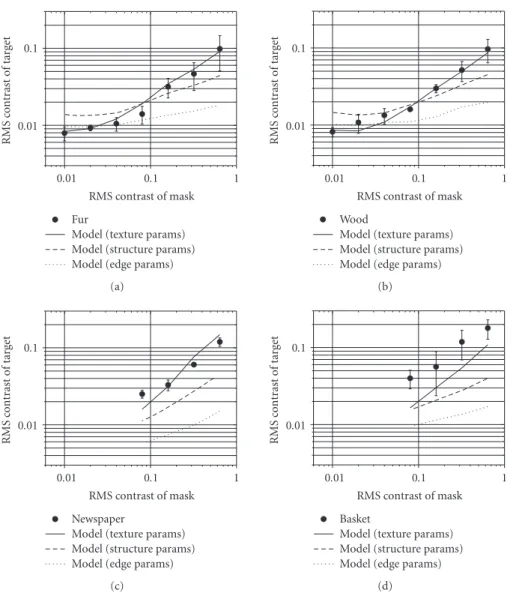
This latter assertion is demonstrated in Figures 12, 13, and 14, which depict model predictions for textures, structures, and edges, respectively, using each set of optimal model parameters. Notice that, as expected, the standard (texture) model performs quite well for textures; in general, the model predictions are within the error bars. Using these same parameters yields reasonably accurate results for structures baby, cat, and flower; however, the predicted thresholds forpumpkinandhandare clearly overestimated in the high-contrast regime. For edges, the standard (texture) model severely overestimates thresholds in the high-contrast regime.

We have experimented with various values of pandb, with generally little eﬀect on model performance if these parameters are set to reasonable (biologically plausible) values. Ifpis adjusted, the optimal value ofqchanges so as to maintain the quantity p-q. Similarly, an optimization in whichbis allowed to vary along withqandg results inb =

0.035, 0.034, and 0.032 for textures, structures, and edges, respectively, and an insignificant change inqandgfrom the values listed in Table 1. Using these optimal values of b as opposed to a fixed value ofb =0.035 results in a negligible eﬀect on model performance for structures and edges. We

have also experimented with a joint optimization of p,q,b, andg, which results in values similar to those listed inTable 1 (while absolute values ofpandqwill vary depending on the initial values of these parameters, the quantity p-qremains consistent).

The model presented here represents an improved ver-sion of a model which we previously proposed in [51]. The primary improvement of our current model over the previous model is that the current model better represents a standard masking model. In particular, our model in [51] took as input pixel-value images as opposed to luminance-value images. The choice of using luminance luminance-values versus pixel values is still debatable, since pixel values more closely correlate with perceived brightness (“lightness” orL∗) [52]. However, the use of luminance is more common in neural modeling, and thus luminance-value images are used in the current model. The model in [51] also used a broad inhibitory pool which consisted of neural responses at all orientations, whereas standard models typically limit the inhibitory pooling over orientation to within ±45◦ of the orientation of the responding neuron [3,4,24], as is used in the current model. In terms of parameter values, our previous model usedp=2.4, as is used in the current model; however, in [51] two diﬀerent values ofqwere used:q=2.75 for textures andq=2.45 for structures and edges; these latter values are nonstandard, since most models, including our current model, employ p > q. In [51], bandg were fixed at b = 0.03 and g = 1, and a new parameter gm (which represented an inhibition modulation term) was employed. In our current model, better fits are achieved without using gm, and instead allowing bothgandqto vary for each image type.

(13)

0.01 0.1

RMS

co

nt

ra

st

of

target

0.01 0.1 1

RMS contrast of mask Fur

Model (texture params) Model (structure params) Model (edge params)

(a)

0.01 0.1

RMS

co

nt

ra

st

of

target

0.01 0.1 1

RMS contrast of mask Wood

(b)

0.01 0.1

RMS

co

nt

ra

st

of

target

0.01 0.1 1

RMS contrast of mask Newspaper

(c)

0.01 0.1

RMS

co

nt

ra

st

of

target

0.01 0.1 1

RMS contrast of mask Basket

(d)

Figure12: Predictions of the gain-control model for textures using parameters optimized for textures (solid line), for structures (dashed line), or for edges (dotted line). The solid circles denote the masking results obtained for each of the textures in the psychophysical experiment.

following section, we demonstrate how adapting a masking model to local image patches can lead to improved results for one common application of masking which is image compression.

4. Application of the Structural Masking Model

to Compression

A wavelet-based image coder that leverages the results of the previous masking study is described in this section. To fully take advantage of the study outlined inSection 2, it is necessary to classify each image patch into one of the three mask types (textures, structures, or edges). Quantization step sizes associated with each patch are derived based on its type and contrast, which jointly make up side information needed by the coder. Explicit as well as implicit compression techniques are applied in order to control the size of a compressed file containing this side information. A block

diagram of the proposed coder is illustrated in Figure 15. Rate-control techniques used to achieve arbitrary target coded rates are also discussed.

(14)

0.01 0.1

RMS

co

nt

ra

st

of

target

0.01 0.1 1

RMS contrast of mask Baby

(a)

0.01 0.1

RMS

co

nt

ra

st

of

target

0.01 0.1 1

RMS contrast of mask Pumpkin

(b)

0.01 0.1

RMS

co

nt

ra

st

of

target

0.01 0.1 1

RMS contrast of mask Hand

(c)

0.01 0.1

RMS

co

nt

ra

st

of

target

0.01 0.1 1

RMS contrast of mask Cat

(d)

0.01 0.1

RMS

co

nt

ra

st

of

target

0.01 0.1 1

RMS contrast of mask Flower

(e)

Figure13: Predictions of the gain-control model for structures using parameters optimized for textures (solid line), for structures (dashed line), or for edges (dotted line). The solid circles denote the masking results obtained for each of the structures in the psychophysical experiment.

side information that must be coded in order to invert the compression process. Thus, a relatively simple rectangular-patch-based approach is used herein that associates a contrast and a type to eachM×Mimage patch. This choice is made for convenience and eﬃciency; mask types and mask contrast values are determined by local, disjoint computations. In order to compensate for the lack of granularity in the segmentation procedure, the contrast of each patch is set to the minimum contrast of all subregions of the patch.

A multistage classifier used to designate each patch as texture, structure, or edge data is described in more detail. A greedy approach to classification is presented. Prior to employing the algorithm, all images patches are labeled as unclassified. During each stage, the classifier selects patches that are associated with only one specific type of mask (texture, structure, or edge content). Only unclassified patches are processed in subsequent stages. Letmindex each patch in the image, letσ2

m denote its variance, and letσm,j2 denote the variance of the jth subpatch of patchm.

(1) The first stage classifies certain patches as edges or textures based on the patch variance. Specifically,

(i) if σ2

m > Kedge× (no. of subpatches such that σ2

m,j> TM), patchmis labeled an edge, or (ii) ifσ2

m > Ktexture×(no. of subpatches such that σ2

m,j> TM), patchmis labeled a texture,

whereKedge,KtextureandTMare constants.

(2) The second stage is composed of three substages, each of which classifies a patch as an edge if a per-patch metric exceeds a threshold similar in form to those used in the first stage. The metrics, in the order in which they are applied, are

(i) average Canny edge-detector output,

(ii) average Laplacian of Gaussian detector output, (iii) variance ofσ2

(15)

0.01 0.1

RMS

co

nt

ra

st

of

target

0.01 0.1 1

RMS contrast of mask Butterfly

(a)

0.01 0.1

RMS

co

nt

ra

st

of

target

0.01 0.1 1

RMS contrast of mask Sail

(b)

0.01 0.1

RMS

co

nt

ra

st

of

target

0.01 0.1 1

RMS contrast of mask Post

(c)

0.01 0.1

RMS

co

nt

ra

st

of

target

0.01 0.1 1

RMS contrast of mask Handle

(d)

0.01 0.1

RMS

co

nt

ra

st

of

target

0.01 0.1 1

RMS contrast of mask Leaf

(e)

Figure14: Predictions of the gain-control model for edges using parameters optimized for textures (solid line), for structures (dashed line), or for edges (dotted line). The solid circles denote the masking results obtained for each of the edges in the psychophysical experiment.

−1

Wavelet coefficient compression Compute

step sizes DWT

DWT DWT

Dead-zone quantize

Code quantized wavelet coefficients

(possibly conditioned on step sizes)

Coded image data Coded classification

map

Entropy code Entropy

decode Dead-zone

dequantize Classification

map

Contrast map

Dead-zone quantize

Entropy code

Coded contrast

map

Side information compression Segmentation

and classification

Image data

Figure15: Block diagram representing the proposed coder. The major components perform segmentation/classification, side information

coding and wavelet coeﬃcient coding. If coding quantized wavelet coeﬃcients conditioned on step size values, more compression gain is

(16)

Table2: Confusion matrix for the example patch type classifier.

Predicted patch type

Texture Structure Edge

Actual patch type

Texture 3450 2137 766

Structure 184 1043 1038

Edge 9 380 1233

(3) The third stage labels all unclassified patches as structures.

This classifier was tuned without using any images in the test set. Performance of this classifier is evaluated in the following way. Ten of the test images were hand-annotated by three expert viewers, classifying each 16×16 block of pixels as a patch of texture, structure, or edge information. This data constitutes a ground truth that can be compared with the classifier. The confusion matrix for the example classifier described above is given inTable 2. In general, the proposed algorithm predicts the correct class in over half the trials. The performance of the classifier can certainly be improved. The main goal of the example coder described herein, however, is to illustrate some of the gains achievable via type-based classification, and the classifier provides enough functionality to accomplish this goal.

After the segmentation and classification phase is com-plete, each patch in the image is associated with a contrast value computed via (3), and a mask type. The set of all patch contrasts, denotedCrms(m), is referred to as acontrast map, and the set of all patch types, denoted type(m), is referred to as aclassification map. Examples of these quantities are illustrated inFigure 16. Samples in the contrast map are from a continuum of values, and elements in the classification map are from a discrete set. Clearly, there is a tradeoﬀbetween the patch size and the amount of auxiliary information produced by this stage. Methods for representing these data eﬃciently are therefore key to the success of utilizing this information.

4.2. Explicit Side Information Coding. In order to generate the step sizes at a decoder, the contrast and classification maps must be conveyed as side information. To improve the eﬃciency of this maneuver, both maps are compressed. The contrast map is compressed in a lossy fashion, and the classification map is losslessly compressed. It is important to perform this compression prior to determining quantization step sizes. Otherwise, the decoder will incorrectly estimate these values during dequantization. The classification map can be represented eﬃciently with an arithmetic entropy coder. Because the contrast map contains relatively low-frequency information (e.g., see Figure 16), a standard wavelet transform coding framework can be used to rep-resent this information economically. A five-level two-dimensional DWT is applied to the contrast map, followed by dead-zone quantization. In doing so, it is important to maintain a high-quality representation of the contrast map, otherwise the perceptual advantage of saving the contrast map is diminished. The compressed contrast map is given by Crms(m). The size of this map must usually be kept

between 2–4 times smaller than the size of uncoded map to achieve this goal. While the explicit coding procedure reduces the overhead associated with the side information, the compressed contrastandclassification maps can still take up a noticeable percentage of the size of the bitstream. An implicit method of rate reduction for the side information is used that is tied closely with the mechanism used to code the quantized wavelet coeﬃcients, and is discussed in Section 4.4.

4.3. Quantization Step Size Computation. Once the

(com-pressed and decom(com-pressed) contrast and classification maps have been established, quantization step sizes for each wavelet coeﬃcient can be derived. With these step sizes, wavelet coeﬃcients in each location are quantized to the threshold of perceived distortion. In other words, the following quantization scheme is designed to createvisually losslessimages. Lossy compression to an arbitrary coded bit rate can also be achieved based on this approach, and is discussed as well.

A quantization step size is derived for each individual wavelet coefficient in each subband as follows. In order to compute this step size, each wavelet coefficient must be associated with a mask type and a contrast value. Because these quantities are computed on a per-patch basis, this assignment proceeds differently depending on the number of coefficients in the subband relative to the patch size. Suppose the image to be compressed is N ×N pixels in size, and that the patch size is M×M pixels. For wavelet subbands with fewer than (N/M) × (N/M) coefficients, there are multiple entries in the contrast map that corre-spond to each wavelet coefficient. In this case, the average contrast computed over all patches corresponding to each coefficient is associated with that coefficient. This operation is conceptually equivalent to resampling the contrast map such that the resampled version is the same size as the wavelet subband. A pictorial representation of this process is illustrated in Figure 17. An analogous method is used to determine contrast values for subbands with more than (N/M)×(N/M) coefficients. Assignment of mask types to each wavelet coefficient proceeds in the same way.

After each wavelet coefficient is associated with a contrast and a mask type, these values are mapped to a set of detection thresholds. CTtype(u0,f0,θ0) denotes the per-type contrast threshold associated with wavelet coefficient x(u0,f0,θ0). The underlying assumption is that if patches of wavelet coefficients are quantized to induce the threshold contrast, the quantization error will be barely visible in the presence of the original image data. The masking model presented earlier can be used for this purpose, but is very computationally intensive. Thus, the following alternative is used for practical reasons. Previous texture masking experiments have demon-strated that TvC curves for images patches with distortions associated with a range of spatial frequencies f [53] can be described with afrequency-adaptivemodel of the form

CTm,f0

=

Hf0

+Crms(m)α(f0) 1/β(f0)

Nf0

(17)

(a) (b) (c)

Figure16: (a) An example imagebug, (b) with a contrast map, and (c) classification map. In the contrast map, dark regions denote low values and light regions denote higher values. In the classification map, black regions denote texture, grey regions denote structure, and white regions represent edges. This information must be transmitted to the decoder.

N×Nimage

(N/M)×(N/M) contrast map

Interpolate for larger subbands Average and

down-sample for smaller subbands

Figure 17: Diagram of relationship between contrast maps and

wavelet subband coeﬃcients. In order to associate each coeﬃcient

in a subband with a contrast value,Crms(u0,f0,θ0) (which is needed

to predict the step size for the coeﬃcient), the contrast mapCrms(m)

is resampled in order to match the number of map entries with

subband coeﬃcients. A similar approach is used to associate each

wavelet coeﬃcient with a patch type.

whereCrms(m) denotes the mask contrast for patchm. This same model is adopted for each patch of coefficients, on a per-mask-type basis. Mask-type-specific TvC data presented herein can be used to fit this model for wavelet subbands with a center spatial frequency of 4.6 cycles/degree; the relative differences between average contrast thresholds for the different frequencies in [53] can be used to derive relationships mapping Crms(u0,f0,θ0) to CTtype(u0,f0,θ0) for different frequencies (and types).

When this value has been computed for each wavelet coeﬃcient, local step sizes may be determined as the step sizes that induce CTtype(u0,f0,θ0) in the distortion image. These values, given byQthreshold₍_u

0,f0,θ0), may be found via iterative bisection search. One diﬃculty with determining Qthreshold₍_u

0,f0,θ0) is that contrast thresholds are measured in the luminance domain. As a result, an iterative approach can be cumbersome. Nevertheless, faster alternatives exist. The contrast threshold can be mapped to an MSE distortion value (using the method described in [53]), and a variety of models for wavelet coeﬃcient data can be used to map this MSE distortion to a step size.

Though the presented experiment and proposed coder yield performance that is optimized for at-threshold (visually lossless) compression, it can be extended to produced coded images at any target rate. The emergence of a number of new rate-control procedures [54,55], which essentially can

be applied on a per-patch basis, yield the ability to do so quickly and accurately. To create coded images at any target rate, the at-threshold step sizes must be modified. One way to do so is the following. Prior to any quantization or coding, each wavelet coefficient is scaled by a spatially-selective weight that is inversely proportional to the step sizes which quantize each coefficient to the threshold of detection. In other words, each wavelet coefficient x(u0,f0,θ0) is first normalized by Qthreshold₍_u

0,f0,θ0), yielding modified coeﬃcients x(u0,f0,θ0) = x(u0,f0,θ0)/Qthreshold(u0,f0,θ0). A traditional (patch-adaptive) MSE-based rate-distortion optimization procedure is carried out to determine step size QMSE(u0,f0,θ0) that will optimally compressx(u0,f0,θ0) at a target rate. Assuming dead-zone quantization where the size of the dead-zone is twice the step size, the final quantization indices are given by

iu0,f0,θ0

= x

u0,f0,θ0

QMSE

u0,f0,θ0

=

_x_u

0,f0,θ0

Qthreshold

u0,f0,θ0

·QMSE

u0,f0,θ0 .

(10)

Note that this operation is equivalent to quantizing the original wavelet coeﬃcients x(u0,f0,θ0) by step sizes

Q(u0,f0,θ0) = Qthreshold(u0,f0,θ0) · QMSE(u0,f0,θ0). A similar approach has been previously used combining a spatially-adaptive quantization scheme with a JPEG-2000 coder [1].

(18)

(a) Baby (b) Beans (c) Bug (d) Casino (e) Duck

(f) Gazebo (g) Geckos (h) Harbour (i) Horse (j) House

(k) Jackal (l) Lander (m) Lena (n) Mill (o) Pelicans

(p) Beans (q) Rainriver (r) Rhino (s) Roommates (t) Seagulls

(u) Stock (v) Sun (w) Temple (x) Wall

Figure18: Test images used to evaluate the proposed coder. These images were chosen to span a range of mask types and contrast content.

used to create each entry. Refinement bits are represented with a simple adaptive arithmetic coder, and sign bits are inserted into the stream as needed uncoded. Though this approach is essentially nonembedded, all fully received subbands in a partially received image can be decoded.

Another alternative that provides a higher level of robustness to bitstream truncation errors is to generate the step sizes, quantize the wavelet data, then simply compress the resulting quantization indices using a more traditional embedded wavelet coder. Several examples of

(19)

(a) (b)

Figure19: (a) Residual images resulting from compressing image

bug using the texture-masking-based approach in [58], and (b)

the proposed structural-masking-based approach, which have been

contrast-enhanced to emphasize diﬀerences.

4.5. Compression Results. To test the proposed method,

images were compressed at visually lossless rates using the proposed method and compared with the an implementa-tion of the coder in [58]. The main diﬀerences between these coders are that (1) the proposed coder requires additional rate to specify the results of the classification stage, such that the decoder can invertibly derive the quantization step sizes from the contrast map, (2) the proposed coder derives step sizes from TvC curves tailored to the mask type of each region (texture, structure, or edge) instead of TvC curves for just for textures, and (3) the proposed coder segments images into 16×16 blocks instead of 8×8 blocks, since content classification, instead of a highly granular segmentation, can be used to ensure appropriate selection of step sizes. Test images consist of twenty-four 512 × 512 8 bit grayscale images, collected from standard databases as well as the Internet, illustrating a range of mask types. These images are illustrated inFigure 18.

4.5.1. Compression Performance. For the tested images, the proposed coder demonstrates a reduction in overall coded rate by an average factor of about 8%. Rates for individual test images are listed in Table 3, as well as the reductions achieved in bits-per-pixel (bpp). Reductions occur for two main reasons: first, the side rate associated with a 16×16 pixel block segmentation is smaller than that associated with an 8×8 pixel block segmentation, and second, the mask-type-specific segmentation results in slightly higher contrast values and thus slightly more aggressive step sizes for certain regions. At the same time, however, the proposed coder spends more bits representing certain regions classified as structures or edges (reflected inFigure 19). The PSNR values in the table corroborate this notion; sometimes the PSNR increases due to finer quantization, whereas sometimes it decreases due to coarser quantization. There are a few examples in which the rate increases. In some cases, this event occurs due to patch classification error; if the model for a patch is not chosen appropriately, coding eﬃciency will be reduced.

4.5.2. Subjective Verification. Results of a perceptual test comparing the two coders involving six of the test images is illustrated in Table 4. Ten nonexpert viewers were pre-sented with both images and asked which was of better quality. On average, 2/3 of the viewers preferred the images created with the proposed method. Figure 19 illustrates a comparison between residuals, which show that the proposed coder places smaller errors in the regions cor-responding to the structures on bug and larger errors in some edge regions that can mask more distortion. The fact that image quality is maintained, even when PSNR decreases, suggests that the proposed coder is making more eﬃcient use of masking properties. We invite interested readers to view the results for all 24 test images at http://foulard.ece.cornell.edu/gaubatz/piv08.

4.5.3. Limitations and Extensions. The proposed nonembed-ded coding scheme has demonstrated the ability to efficiently represent an image despite the side information to specify highly spatially adaptive perceptual quantization parameters. Still, it does not result in a fully scalable image representation. It is more difficult to take advantage of the side information for implicit rate gain when representing the data in a finely layered fashion. The far right column in Table 3 illustrates this effect for the tested images. Creating a fully-scalable representation results in an increase in coded image size of roughly 0.01 to 0.04 bpp.

5. Conclusions

In this paper, we have advocated for the use of a patch-based structural masking model in which neural modeling is coupled with a classification scheme that selects appropriate model parameters based on the type of structural content (texture, structure, and edge) contained in local image patches.

The results of a psychophysical masking experiment using masks consisting of natural-image patches revealed that the ability of an image patch to mask wavelet subband quantization distortions depends not only on mask contrast, but also on whether the mask is a texture, structure, or edge. As previous masking studies have found, our results revealed that detection thresholds increase as the contrast of the mask increases. For very low mask contrasts of 0.01, 0.02, and 0.04, detection thresholds were similar for textures, structures, and edges. However, the thresholds for the three types demonstrated a marked divergence as the contrasts of the masks increased. High-contrast textures elevated detection thresholds approximately 4.3 times over those for high-contrast edges, and high-contrast structures elevated thresholds approximately 2.6 times over those for high-contrast edges. These results demonstrate that a proper measure of masking in images should account both for local contrast and for local image content.