Artificial Bee Colony algorithm for Localization in Wireless Sensor Networks
S.Sivakumar
Assistant Professor (Selection Grade), Department of ECE, PSG College of Technology, Coimbatore, India. E-mail: [email protected]
Article Received: 10 March 2017 Article Accepted: 19 March 2017 Article Published: 20 March 2017
1.INTRODUCTION
Wireless Sensor Network (WSN) is a kind of ad hoc network that consists of autonomous sensors with low cost, low energy sensing devices, which are connected by wireless communication links. These sensor nodes are tiny in size and possess limited resources namely processing, storage, sensing and communication [1]. They are usually deployed in large numbers over the region of interest for object monitoring and target tracking applications. The densely deployed sensors are expected to know their spatial coordinates for effective and efficient functioning of WSNs. Location awareness is significant for high-level WSN applications like locating an enemy tank in a battlefield, locating a survivor during a natural calamity and in certain low-level network applications like geographic routing and data centric storage.
Localization is a fundamental problem which can be defined as the process of finding the position of the sensor nodes or determination of spatial coordinates of the sensor nodes. Localization is especially important [2] when there is an uncertainty on the exact location of fixed or mobile devices. Localization is the process of making every sensor node in the sensor network to be aware of its geographic position [3]. The usual solution is to equip each sensor with a GPS receiver that can provide the sensor with its exact location. As WSNs normally consist of a large number of sensors, the use of GPS is not a cost-effective solution and also makes the sensor node bulkier [4]. GPS has limited functionality as it works only in open fields and cannot function in underwater or indoor environments. Therefore, WSNs are required of some alternative means of localization.
Currently the existing non-GPS based sensor localization algorithms [5] are classified as range-based or range-free. Range-based localization schemes rely on the use of absolute
point-to-point distance or angle estimate between the nodes to determine the position of unknown sensor nodes using some location-aware nodes. Location-aware nodes are also called as anchors or beacons. Typical range-based localization techniques used are Received Signal Strength Indicator (RSSI) [6], Time Difference of Arrival (TDoA) [7], Time of Arrival (ToA) [8], and Angle of Arrival (AoA) [9]. Depending on the signal feature used, the position estimation is found using geometrical approaches such as Triangulation, Trilateration or Multilateration. Range-based methods give fine-grained accuracy but the hardware used for such methods are expensive. In range-based mechanisms, the nodes obtain pair wise distances or angles [10] with the aid of extra hardware providing high localization accuracy. Due to cost, the use of range-based methods will not be preferred.
Range-free or proximity based localization schemes rely on the topological information, e.g., hop count and the connectivity information, rather than range information. Range-free localization schemes may or may not be used with anchors or beacons. These schemes do not involve in the use of complex hardware and are cheaper when compared to range-based schemes. Range-free methods use the content of messages from anchor nodes and other nodes to estimate the location of non-anchor (unknown sensor) nodes. Centroid Algorithm [11] and Distance Vector Hop (DV-Hop) method [12] are certain range-free algorithms. Range-free algorithms sometimes use mobile anchors [13] for localization. Range-free algorithms are not costly but they provide coarse-grained accuracy.
Localization in Wireless Sensor Networks is intrinsically an unconstrained optimization problem [14]. Localization can be viewed as an NP-hard optimization problem. Evolutionary algorithms are local search methods, capable of efficiently A B S T R A C T
Localization in wireless sensor networks (WSNs) is one of the most important fundamental requisite that needs to be resolved efficiently as it plays a significant role in many applications namely environmental monitoring, routing and target tracking which is all location dependent. The main idea of localization is that some deployed nodes with known coordinates termed as anchor nodes transmit beacons with their coordinates in order to help the other nodes in the sensing field to localize themselves. Broadly there are two types of localization methods used for calculating positions namely the range-based and range-free methods. Initially, a range-free localization algorithm namely, Mobile Anchor Positioning - Mobile Anchor & Neighbor (MAP-M&N) is applied. In this algorithm, the sensor nodes use the location information of beacon packets of mobile anchor nodes as well as the location packets of neighboring nodes to improve the accuracy in localization of the sensor nodes. In this paper, the proposed optimization approach is Artificial Bee Colony (ABC) algorithm which is incorporated with MAP-M&N to further improve the accuracy in positioning the sensor nodes. The objective of this work is to compare the performance of MAP-ABC approach with regard to MAP-M&N algorithm. Root Mean Square Error (RMSE) is the performance metric to compare between the two approaches namely, MAP-M&N and MAP-ABC algorithms. A study on average localization error and comparison between the two approaches namely, MAP-M&N and MAP-ABC has been done. Simulation results reveal that Artificial Bee Colony approach used along with MAP-M&N outperforms by minimizing error in when compared to using only MAP-M&N approach for localization.
solving complex constrained or unconstrained optimization problems.
The rest of the paper reviews the related research work in this area, elaborates the Mobile Anchor Positioning (MAP) method and the proposed Artificial Bee Colony Optimization with Mobile Anchor Positioning (MAP-ABC) and compares the performance of the proposed approach with MAP-M&N.
2. RELATED WORK
W-H Liao et al. [15] proposed an algorithm, Mobile Anchor Positioning in which each sensor node receives beacons (messages containing location information) in its receiving range from the moving anchor as the anchor moves around the sensing field. Among the received beacons, the sensor node selects the farthest two beacons. The node constructs two circles with each chosen beacon as centre. The radius of the circle is the communication range of the sensor node. It determines the intersection points of the two circles. Out of the two points, one is chosen to be the location of the sensor node based on a decision strategy.
Kuo-Feng Ssu et al. [16] presented a range-free algorithm, which uses the following conjecture. A perpendicular bisector of a chord passes through the centre of the circle. When there are two chords of the same circle, their perpendicular bisectors will intersect at the centre of the circle. A mobile anchor moves around the sensing field broadcasting beacons. Each sensor node chooses two pairs of beacons and constructs two chords. The sensor node assumes itself as the centre of a circle and determines its location by finding the intersection point of the perpendicular bisectors of the constructed chords.
Baoli Zhang et al. [17] proposed a range-free algorithm, which works as follows. The trajectories of the mobile anchor are in such a way that it moves in a straight line. As it moves, it periodically broadcasts its location to the sensor nodes. A sensor node selects four beacons among all collected beacons. The first group (two beacons) is the location of the mobile anchor node when it first enters the communication range of the sensor node. The second group is the location of the mobile anchor node when it second enters the communication range of the sensor node. After these positions and the communication range are obtained, four circles are constructed with the chosen four points as centers. Four intersection points s1, s2, s3, s4 of the circles are calculated. Then using the centroid formula on the four intersection points, the position of the sensor node is calculated.
Wenwen Li et al. [18] proposed the Genetic algorithm for localization of the sensor nodes and constructed the solution space, coded the solutions, formulated the fitness function and used appropriate selection mechanism to choose the parents for the next generation. The reproduction operation on the individuals is further performed and the solution is obtained with high accuracy. The above genetic algorithm approach gives good localization accuracy but the solution space is very huge. The algorithm has to search a large number of solutions in each of the iterations or the number of iterations will be
large. When the area of the sensing field increases, the computation involved also increases.
Gopakumar et al. [19] proposed the swarm intelligence based approach for localization of the sensor nodes for this non-linear optimization problem. The objective function chosen is the mean squared range error of all neighboring anchor nodes. The PSO algorithm provides better convergence than simulated annealing and ensures solution without being trapped into local minima.
Lutful Karim et al. [20] proposed a Range-free Energy Efficient Localization Technique using Mobile Anchor (RELMA) especially for large scale WSNs to improve both accuracy and energy efficiency by minimizing the number of anchor nodes used. The performance of RELMA_Method 1 and RELMA_Method 2 are compared only with the existing Neighboring-Information-Based Localization System (NBLS). Simulation results demonstrate the fact that RELMA_Method 1 and RELMA_Method 2 outperform NBLS in terms of localization accuracy as well as energy efficiency.
Xu Lei et al. [21] proposed a Mobile Anchor Assisted Localization Algorithm based on PSO (MAAAL_PSO) pertaining to adverse or dangerous application environments. The Region of Interest (ROI) is divided into grids and the mobile anchor deploys virtual anchors on the vertex of each grid. Based on this deployment, the node localization is converted into non-linear constrained optimization problem solved by PSO with the help of mobile anchor. After a few iterations, performance evaluations demonstrate that this algorithm improves localization accuracy. It is also robust to the interference of environment noise.
The proposed optimization algorithm in this paper is Artificial Bee Colony, which is applied along with Mobile Anchor Positioning (MAP-ABC). Here the location of nodes is initially estimated by MAP-M&N. Then ABC algorithm is applied over the results of MAP-M&N. It is observed that MAP-ABC approach provided relatively much better accuracy than MAP-M&N.
3. PROPOSED LOCALIZATION APPROACH
The localization strategy used in this work can be visualized to work in two stages. In the first stage, Mobile Anchor Positioning - Mobile Anchor & Neighbor (MAP-M&N) is used for determining the location of the unknown sensor nodes. Since a range-free algorithm offers only coarse-grained accuracy, the obtained location will be just as an estimate. In the second stage (post optimization stage), proposed Artificial Bee Colony (ABC) algorithm is applied over MAP-M&N algorithm for fine-tuning the results of the sensor nodes obtained using MAP-M&N and thereby improving localization accuracy.
3.1. Mobile Anchor Positioning (MAP)
field fitted with Global Positioning System (GPS). As they move around the sensing field, they periodically broadcast beacons containing their current location at fixed time interval to all the nodes, which are at a hearing distance from it. The mobile anchors traverse around the field with a specific speed and their directions are set to change for every ten seconds. All the nodes in the communication range of the mobile anchor will receive the beacons. A sensor node will collect all the beacons in its range and store it as a list. The assumption made is that the communication range of the sensor node and the mobile anchor node are the same. Once enough beacons are received and if a sensor node does not receive a beacon, which is at a distance greater than the already received ones, the localization begins at that particular node.
Assume that the sensor node has received and stored four beacons (locations of the mobile anchor) in its list {T1, T2, T3, and T4} as shown in Fig. 1. From the list, two beacons, which are farthest from each other, are chosen (T1, T 4). These points are known as Beacon points. These two points are marked as the end of the sensor node’s communication range since the sensor node has not received a beacon farther from this point. Hence T1 and T4 (Beacon points) represent either two positions of the same mobile anchor or positions of two different mobile anchors when they were at the end of the sensor node’s communication range.
With these two Beacon points as centers and the communication range of a sensor node as radius, two circles are constructed (refer Fig.1). Each circle represents the communication range of the mobile anchor, which has sent the beacon. The sensor node has to fall inside this communication range, as it has received the beacon. Since the sensor node has received packets either from both anchors or from the two positions of the same anchor, the node has to fall inside both the circles. Hence, it can be concluded that circles will intersect each other.
Fig.1. Possible Locations of the Sensor Node
The intersection points of both circles are determined (S1, S2). The intersection points are the possible locations of the sensor node. The reason is as follows: The two farthest points (Beacon points) are the end points of a sensor node’s communication range. The sensor node lies on the circumference of the other circle since it is the same with the other mobile anchor position. Therefore, the sensor node lies on the circumference of both the circles. The only points satisfying the above condition are the two intersection points.
Hence, by means of Mobile Anchor Positioning, the location of the sensor node has been approximated to two locations.
3.1.1 Identifying the Sensor Locations using MAP with Mobile Anchor (MAP-M)
The visitor list is searched after identifying the two possible positions i.e. the intersection points. If a node could hear around its range, there is a possibility of a beacon point which can be situated at a distance r from one of the two possible locations. Thus, there is one point in the list, whose distance from one possible location is less than r, and the distance from other possible location is greater than r, then the first possible location is chosen as the location of the sensor node.
It is assumed that the communication range of a mobile anchor is R. The MAP-M maintains the visitors list after receiving the beacon packets from the mobile anchor. The information from the visitor list is used to approximate the location of the sensor node. Let the visitor list of a sensor node S consists of various location information represented as {T1, T2… Tn}. The beacon points are the two extreme points i.e., T1 and Tn. Two circles with radius R and center T1 and Tn are constructed and their intersection points of two circles are found to be S′ and S′′. If there is any Ti (2 ≤ i ≤ n-1), such that the distance between Ti and S′ is less than R and that between Ti and S′′ is greater than R, then we can conclude the location of the sensor node is S′. This is because of the fact that the sensor node should lie inside the communication range of mobile anchor to receive the beacon packets. Consequently, the distance between the sensor node S and beacon packet Ti should be less than R.
Fig. 2. Node Seeking Information from Neighbor Sensors
obtained, then a single position of sensor node S cannot be obtained. The node will have two positions S' and S" as shown in Fig. 2. To overcome this problem, the method of Mobile Anchor Positioning-Mobile Anchor & Neighbor (MAP-M&N) is being adopted.
3.1.2 Forming additional Anchors and identifying the Sensor Locations using MAP with Mobile Anchor & Neighbor (MAP-M&N)
The location estimation done for sensors using MAP-M method gives positions for few sensors and for the others, it gives two positions and therefore it is the responsibility of MAP-M&N method to produce outputs with a single position for each sensor.
It is possible for the sensor nodes that have already determined their location to assist other nodes in determining their locations. As soon as the location is identified, the localized nodes start acting like anchors. They embed their calculated location inside the packet and then broadcast the beacons.
Nodes, which are at its hearing range and waiting for additional beacons to finalize their location, can make use of these beacons. However, if the sensor node has determined its location, it simply discards the beacon packet. By using MAP-M&N method, the cost of movement of the mobile anchor can be reduced.
The steps in finding the location of the sensors in the field using MAP – M & N method are the following:
1. Deploy 100 sensor nodes randomly in the 1000 m x 1000 m area of the sensing field in the simulation environment and deploy 3 location aware nodes (anchor nodes) i.e. sensor nodes fit with GPS.
2. The assumption made is that Mobile Anchors move throughout the sensing field according to the positional data specified in the movement file which is given as input to the NS2 simulator. The anchor nodes periodically broadcast their location packets, which are known as beacon packets, while on the move through the sensing field.
3. Every sensor node maintains a visitor list containing beacon packets based on the information obtained from anchors.
4. The sensor nodes can identify the farthest beacon packets and chooses those beacon packets as beacon points.
5. With those two beacon points as the centers and the communication range of a sensor node as radius, two circles are constructed and the intersection points are found.
6. Sensor nodes try to identify its position out of the two intersection points. Here, at least one of the beacon points in the visitor list must lie outside the shadow region or based on the beacon points obtained from neighbor nodes.
7. The approximate location for each of the sensor nodes is estimated using the MAP-M&N method.
3.2 Mobile Anchor Positioning with Artificial Bee Colony
(MAP-ABC) Optimization Algorithm
The Artificial Bee Colony Optimization (ABC) [22] algorithm can be applied for solving optimization problems. Here ABC algorithm takes the results of MAP-M&N as the input. The localization steps used in ABC algorithm are the following:
1. The algorithm takes the results of MAP-M&N as its input. The results of MAP-M&N, giving the approximate solution of the location of each sensor at each specified time instance is given as the input to the post optimization method.
2. Let m be the number of sensor nodes randomly placed for each food source xi of employed bees using Eq. (1).
xij = minj + rand(0, 1)( maxj − minj) (1)
3. Now evaluate the position of the food source using employee bees.
4. Produce new solutions υi in the neighborhood of xi for the employed bees using Eq. (2)
vij = xij + φij(xij - xkj) (2)
Here, k is a solution in the neighborhood of i, φ is a random number in the range [-1, 1], and j is the randomly selected mobile sensor’s position.
5. Check υij for staying in the bounds of the area and apply the greedy selection process between xi and υi.
6. After applying the greedy selection process for the sensor nodes visited by the employee bees calculate the fitness value for the sensor nodes.
7. Calculate probability values Pi for solutions xi by means of their fitness values using Eq. (3).
Pi = [ 0.9 * (fiti / Fitbest) ] + 0.1 (3)
Here fiti is the fitness value of ith solution and Fitbest is the maximum fitness of the solutions.
8. Produce the new solutions, υi, for the onlooker bees from solutions xi, selected depending on Pi, and deploy the onlooker bees onto the respective food source.
9. Apply the greedy selection process for the onlookers between xi and υi, until the position of the food source is accurately found.
11. Determine the abandoned solution and deploy the scout bees to find new food sources so as to find its position.
12. Repeat the procedure until the stopping criteria is met. Stopping criteria = Maximum iterations or Profit value Maximum iteration = arbitrarily chosen as 100.
4. SIMULATION RESULTS
The simulation settings used in ns-2 simulator for localization using proposed approach when compared to MAP-M&N algorithm is as shown in Table I.
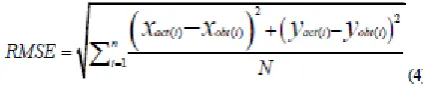
4.1 Metric used to determine Localization Accuracy The metric that is used to evaluate the localization accuracy is Root Mean Square Error (RMSE). Equation (4) gives the RMSE formula for the proposed evolutionary approaches,
Where, xact ( i), yact ( i) - represent the actual values of x and y coordinates of the sensor nodes, xobt ( i) , yobt ( i ) - represent the obtained values x and y coordinates of the sensor nodes and N - represents the total number of Localized nodes.
4.1.1 Comparison of RMSE obtained using MAP-M&N and MAP-ABC approaches
The accuracy in localization can be evaluated based on minimization in positional error. Root Mean Square Error (RMSE) is calculated for MAP-ABC and MAP-M&N approaches pertaining to every ten nodes scenario as listed in Table II. The Table II shows the RMSE analysis of MAP-ABC and MAP-M&N approaches corresponding to 10, 20, 30 etc. up to 100 nodes scenario which illustrates clearly that RMSE gets drastically reduced on an average when Artificial Bee Colony algorithm is used with MAP-M&N algorithm (MAP-ABC) when compared to using only MAP-M&N algorithm.
Table I: Simulation Settings
From the simulation results based on RMSE in Table II, it can be summarized that the proposed Artificial Bee Colony with Mobile Anchor Positioning (MAP-ABC) algorithm
minimizes the percentage of localization error significantly by 95.70 % when compared to using only MAP-M&N algorithm on an average for 100 nodes scenario.
Table II: RMSE obtained for MAP-M&N and MAP-ABC approaches
5. CONCLUSION
Mobile Anchor Positioning with Mobile Anchor & Neighbor (MAP-M&N) algorithm uses range-free localization mechanism that does not involve usage of any hardware. The percentage of localized nodes is high which indicates that MAP-M&N is appropriate for localization. Since this method does not give fine-grained accuracy, Population based optimization technique namely Artificial Bee Colony algorithm is applied over the results of MAP-M&N. From the simulation results based on RMSE, Mobile Anchor Positioning with Artificial Bee Colony (MAP-ABC) algorithm minimizes the percentage of localization error significantly by 95.70 % when compared to MAP-M&N algorithm on an average.
Thus, it is concluded that MAP-ABC algorithm minimizes the localization error better than MAP-M&N. Hybridization of optimization namely Simulated Annealing (SA) can be combined to Mobile Anchor Positioning with Artificial Bee Colony algorithm (MAP-ABC-SA) so as to reduce the localization error further and the localization error of the hybrid evolutionary algorithm can be compared with the pure ABC algorithm (MAP-ABC) to validate its performance. The future enhancement may be applying meta-heuristic optimization approaches such as Glow worm swarm optimization, fish swarm optimization etc. with mobile anchor positioning to further minimize the localization error significantly in wireless sensor networks.
REFERENCES
[1] I.F.Akyildiz, W.Su, Y. Sankarasubramanium, and E. Cayirci, “Wireless sensor networks: A Survey,” IEEE Computer., vol. 38, Issue 4, pp.393 – 422, 2002.
[2] Jonathan Bachrach and Christopher Taylor, Localization in Sensor Networks, Chapter 9, Ivan Stojmenovic, Handbook of Sensor Networks: Algorithms and Architectures, 2006, pp. 277-297.
[4] Guibin Zhu, Qiuhua Li, Peng Quan, and Jiuzhi Ye, “A GPS-free localization scheme for Wireless Sensor Networks,” Proc. of the 12th IEEE Int. Conf. on Communication Technology (ICCT 2010), pp. 401-404, Nov 2010.
[5] C.Zenon, K.Ryszard, N.Jan, and N.Michal, “Methods of sensors localization in wireless sensor networks,” Proc. of the 14th Annual Int. Conf. and Workshops on Engineering on Computer based Systems (ECBS 2007), pp. 145-152, Mar 2007.
[6] Hoang Q.T., Le T.N., and Yoan Shin, “An RSS comparison based localization in wireless sensor networks,” 8th workshop on Positioning Navigation and communication (WPNC 2011), pp.116-121, April 2011.
[7] Pengfei Peng, Hao Luo, Zhong Liu, and Xiongwei Ren, “A cooperative target location algorithm based on time difference of arrival in wireless sensor networks,” Proc. of the Int. Conf. on Mechatronics and Automation (ICMA 2009), pp. 696-701, Aug 2009.
[8] Guowei Shen, Zetik R, Honghui Yan, Hirsch O, and Thoma R.S., “Time of arrival estimation for range-based localization in UWB sensor networks,” Proc. of the IEEE Int. Conf. on Ultra-Wideband (ICUWB 2010), vol. 2, pp. 1-4, Sep 2010.
[9] Y.Zhu, D.Huang, and A.Jiang, “Network localization using angle ofnarrival,” Proc. of the IEEE Int. Conf. on Electro/Information Technology (EIT 2008), pp. 205-210, May 2008.
[10] G.Yu, Fengqi Yu, and L.Feng, “A localization algorithm using a mobile anchor node under wireless channel,” Proc. of IEEE Int. Conf. on Robotics and Biomimetics, Dec 2007.
[11] B.Deng, G.Huang, L.Zhang, and H.Liu, “Improved centroid localization algorithms in WSNs,” Proc. of the 3rd Int. Conf. on Intelligent System and Knowledge Engineering (ISKE 2008), vol. 1, pp. 1260-1264, Nov 2008.
[12] Zhang Zhao-yang, Gou Xu, Li Ya-peng, and Shan-shan Huang, “DV Hop based self-adaptive positioning in wireless sensor networks,” Proc. of the 5th Int. Conf. on Wireless Communications, Networking and Mobile Computing (WiCom 2009), pp. 1-4, Sept. 2009.
[13] Patro, R.K, “Localization in wireless sensor network with mobile beacons,” Proc. of the 23rd IEEE convention of Electrical and Electronics Engineers, Israel, pp. 22-24, Sept. 2004.
[14] Q. Zhang, J. Wang, C. Jin, and Q. Zeng, “Localization algorithm for wireless sensor network based on genetic simulated annealing algorithm,” Proc. of the IEEE Int. conf. on Wireless Communications, Networking and Mobile Computing, 2008.
[15] W-H Liao, Y.C.Lee, and S.P. Kedia, “Mobile anchor positioning of wireless sensor networks,” IET communications, vol. 5, issue 7, pp.914-921, 2011.
[16] Kuo-Feng Ssu, Chia-Ho Ou, and H.C. Jiau, “Localization with mobile anchor points in wireless sensor networks,” IEEE Transactions on Vehicular Technology, vol. 54, no. 3, May 2005.
[17] B.Zhang, Fengqi Yu, and Zusheng zhang, “An improved localization algorithm for wireless sensor network using a mobile anchor node,” Asia-Pacific Conference on Information Processing, 2009.
[18] Wenwen Li and Wuneng Zhou, “Genetic Algorithm - Base Localization Algorithm for Wireless Sensor Networks,” Proc. of the 7th Int. Conf. on Natural Computation (ICNC 11), pp. 2096-2099, July 2011.
[19] Gopakumar.A and Jacob.L, “Localization in wireless sensor networks using particle swarm optimization,” Proc. of the IET Int. Conf. on Wireless, Mobile and Multimedia Networks, pp. 227-230, 2008.
[20] L.Karim, N.Nasser, and T.El Salti, “RELMA: A range free localization approach using mobile anchor node for wireless sensor networks,” Proc. of IEEE Globecom, 2010.
[21] X.Lei, Z.Huimin, and S.Weiren, “Mobile anchor assisted node localization in sensor networks based on particle swarm optimization,” Proc. of IEEE WiCom, 2010.