Hyperspectral Image Classification using Genetic Algorithm after Visualization using Image Fusion

Hyperspectral Image Classification using Genetic

Algorithm after Visualization using Image Fusion

1

B.Saichandana,

K.Srinivas,

R.Kiran Kumar

1_{Dept. of CSE, GIT, GITAM University, Visakhapatnam, Andhra Pradesh, India} 2Dept. of CSE, VR Siddhartha Engineering College, Vijayawada, Andhra Pradesh, India

3Dept. of CS, Krishna University, Machilipatnam, Andhra Pradesh, India Abstract

This paper presents hyperspectral image classification using genetic algorithm after visualization using image fusion technique. Hyperspectral remote sensors collect image data for a large number of narrow, adjacent spectral bands. Every pixel in hyperspectral image involves a continuous spectrum that is used to classify the objects with great detail and precision. In this paper, first 2-D Empirical mode decomposition method is used to remove any noisy components in each band of the hyperspectral data. After filtering, band selection method is performed to select specific bands from the hyperspectral data, in-order to reduce redundancy between bands and to eliminate bands with less information. After band selection, image fusion is performed on the selected hyperspectral bands to selectively merge the maximum possible features from the images to form a single image. This fused image is classified using genetic algorithm. Two different indices, such as K-means Index (KMI) and Jm measure are used as objective functions. This method increases classification accuracy of hyperspectral image.

Keywords

Image Classification, Empirical Mode Decomposition, Genetic Algorithm, Hyperspectral Image

I. Introduction

The process of acquiring information about an object on the earth using satellites without making any physical contact is called remote sensing [1]. The classification of objects on the earth by using electromagnetic radiations reflected or emitted by the surface is the main goal of remote sensing technology [2]. New opportunities to use remote sensing data have arisen, with the increase of spatial and spectral resolution of recently launched satellites. Image classification is a key step in remote sensing applications. In remote sensing, sensors are available that can generate hyperspectral data, involving many narrow bands in which each pixel has a continuous reflectance spectrum. Unsupervised image classification is an important research topic in hyperspectral imaging, with the aim to develop efficient algorithms that provide high classification accuracy.

The hyperspectral images suffer from noises due to disturbance of transmission medium in the atmosphere or degradation of sensors etc leading to affect the accuracy of classification algorithms. This paper presents hyperspectral image classification using EMD and Image fusion. 2-D Empirical mode decomposition method is used to divide the hyperspectral image belonging to a specific band into finite number of components called intrinsic mode functions. The last component is called a residue. The first IMF is filtered using uniform kernel filter (averaging or mean filter). The summation of filtered IMF and remaining IMFs plus residue gives the de-noised image. The same procedure is repeated for all the bands. After filtering band selection technique is used to reduce the redundancy of spectral information without losing valuable details in the data set. After band selection, the bands are fused into a single image

for application oriented visualization, effective interpretation, extraction of useful features, and to provide a better description of the scene using reduced data sets. After fusion, the image is classified using genetic algorithm with two different objective functions. This method increases the classification accuracy both in qualitative and quantitative analysis.

This paper is structured as follows: section II presents filtering using bi-dimensional empirical mode decomposition, section III presents band selection technique, section IV presents image fusion technique, section V presents Genetic algorithm for image classification, section VI shows experimental results and section VII report conclusions.

II. Empirical Mode Decomposition

Empirical mode decomposition [5] is a signal processing method that nondestructively fragments any non-linear and non-stationary signal into oscillatory functions by means of a mechanism called shifting process. These oscillatory functions are called Intrinsic Mode Functions (IMF), and each IMF satisfies two properties, (a) the number of zero crossings and extrema points should be equal or differ by one. (b) Symmetric envelopes (zero mean) interpret by local maxima and minima [6]. The signal after decomposition using EMD is non-destructive means that the original signal can be obtained by adding the IMFs and residue. The first IMF is a high frequency component and the subsequent IMFs contain from next high frequency to the low frequency components. The shifting process [7] [12] used to obtain IMFs on a 2-D signal (image) is summarized as follows:

Let I(x,y) be a Image used for EMD decomposition. Find all •

local maxima and local minima points in I(x,y).

Upper envelope Up(x,y) is created by interpolating the •

maxima points and lower envelope Lw(x,y) is created by interpolating minima points. This interpolation is carried out using cubic spline interpolation method.

Compute the mean of lower and upper envelopes denoted •

by Mean(x,y).

( ( , ) ( , )) ( , )

2

Up x y Lw x y

Mean x y = + (1)

This mean signal is subtracted from the input signal. •

Sub x y( , )=I x y Mean x y( , )− ( , ) (2) If Sub(x,y) satisfies the IMF properties, then an IMF is •

obtained .

IMF x y_{i( , )}=Sub x y_{( , )} (3) Subtract the extracted IMF from the input signal. Now the •

value of I(x,y) is

I x y( , )=I x y IMF x y( , )− i( , ) (4)

This process is repeated until I(x,y) does not have maxima or minima points to create envelopes. Original Image can be reconstructed by inverse EMD given by

1

( , )

( , )

( , )

i

I x y

IMF x y res x y

=

=

∑

+

Image Denoising using EMD:

The mechanism of de-noising using EMD is summarized as follows

Apply 2-D EMD for each band in the hyper spectral image to •

obtain IMFi (i=1, 2, …, k). The kth IMF is called residue. The first intrinsic mode function (IMF1) contains high •

frequency components and it is suitable for denoising. This IMF1 is denoised with This IMF1 is de-noised with uniform filter. This de-noised IMF1 is represented with DNIMF1. The new band is reconstructed by the summation of FIMF •

and remaining IMFs given by

2

1 k i

i

RI DNIMF IMF

=

= +

∑

Where RI is the reconstructed band.

III. Band Selection Technique

Hyperspectral image bands are the result of sampling a continuous spectrum at narrow wavelength intervals where the nominal bandwidth of a single band is 10 nm [9]. The spectral response of the scene varies gradually over the spectrum, and thus, the successive bands in the hyperspectral image have a significant correlation. The dimensionality of the hyperspectral data set strongly affects the performance of any unsupervised classification algorithm. Some of the bands contain redundant data and some contain less discriminatory information between others. In-order to process this high dimensional data, many requirements such as storage space, computational load, communication bandwidth etc is imposed on the classification algorithm. Therefore it is advantageous to remove bands that convey less information. The band selection is done according to any of these following metrics

1. Euclidean Distance (ED) [18]: It is vector distance measurement between any two vectors, defined as

2

1

( , ) N ( _{k k}) k

ED X Y X Y

=

=

∑

Where X and Y are two vectors and Nb denotes the number of bands.

2. Spectral Angle Mapper (SAM) [19]: It is a vector angle measurement between any two vectors, defined as

. ( , ) arccos( )

. T X Y SAM X Y

X Y

= ₍₈₎

Where X and Y are two vectors and Nb denotes the number of bands.

3. Spectral Correlation Mapper (SCM) [20]: It is a vector correlation measure that measures the strength of the linear relationship between two vectors, defined as

(9)

Where X and Y are two Nb dimensional spectral vectors and μ denotes the mean and σ denotes the standard deviation of corresponding vector.

For ED and SAM bands with larger values are selected and for SCM bands with smaller values are selected.

IV. Image Fusion of Selected Hyperspectral Bands

The hyperspectral data present abundant multidimensional information that contains far more image bands than those that can be displayed on the standard tristimulus display. Therefore, an efficient and appropriate means of visualization of the hyperspectral data is needed [8]. Let us consider I₁, I₂, …. I_k be a set of hyperspectral bands, containing K consecutive bands. From these K consecutive bands, only few bands are selected based on the band selection technique. We want to fuse these selected bands to generate a high contrast resultant image for visualization. The primary aim of image fusion is to selectively merge the maximum possible features from the source images to form a single image. Therefore, for an efficient fusion, we should be able to extract the specific information contained in a particular band [13]. The fused image F can be represented as a linear combination of selected images Ik, k = 1 to M as shown below:

1

1

( , )

( , ) ( , )

( , ) 1, ( , )

M k k k M i k

F x y

w x y I x y

and

w x y

x y

=

=

=

= ∀

∑

∑

where wk (x, y) is the weight for the pixel at location (x, y) in the k-th observation, F(x,y) is the fused image and the sum of all weights at any spatial location equals unity, i.e., normalized weights.

V. Genetic Algorithm

Genetic Algorithms [14] belong to the class of evolutionary algorithms that are based on principles of natural selection and genetics. It is a search technique used in computing true solutions to optimization problems that is driven by natural evolution process. GA performs parallel search of the solution space rather than point by point search. Genetic Algorithm consists of three operators namely, Selection, Crossover and Mutation.

The Genetic Algorithm mechanism can be abstracted as follows [15].

The initial population of solutions is randomly generated 1.

across the search space.

Using an objective function, the fitness of each individual 2.

solution in the population is evaluated.

Using this fitness values, the solutions in the population are 3.

selected.

New population is created from selected solutions using the 4.

crossover and mutation operators.

The new population is replaced instead of old population. 5.

Repeat iteratively from (2) to (5) until a stop criterion 6.

is satisfied. Each iteration of this GA process is called generation.

GA is a method of parallel search of the solution space based on two assumptions inspired by evolutionary biology.

The measure of problem solving ability by an individual in •

the population is determined by its fitness value.

individuals in the population have more problem solving ability.

A. Image Classification using GA:

The Genetic Algorithm is applied as follows.

Assume P chromosomes in the population where P is the size •

of the population. Each chromosome is encoded with K cluster centers that are randomly selected from the image.

Using an objective function, the fitness value of each •

chromosome is evaluated. Three Different indices, such as K-means Index (KMI) and Jm measure are used as objective functions individually. For computing the measures, the

centers z₁, z₂, …., z_k encoded in a chromosome are first

extracted. The membership values u_ik, i=1,2,….K and

k=1,2,….n are computed [10] as follows:

(11)

Where D(z_i, x_k) is the Euclidean distance between two points x_k and cluster center z_i.

The centers encoded in a chromosome are updated using the following equation:

(12)

The J_m measure [16] which is to be minimized is defined as

(13)

Where m is the fuzzy exponent, D denotes the Euclidean distance

between two points x_j and z_k and u_kj denotes the membership

values.

The k-means index [17] which is used as the objective function in this GA process is defined as follows:

2 1 1 1 K N i k k i KMI x z = = = −

∑∑

Where K number of clusters and z_k is the cluster centers

The selection of chromosomes is done based on the fitness •

value using roulette wheel technique.

By applying crossover and mutation operators with rate 0.8 •

and 0.07, a new population is produced from the parents. This new population replaces the old population.

Maximum number of iterations is used as stopping criteria. •

After the execution stops, the highest fitness value chromosome is selected and the values in this chromosome represent the solution to the classification of image.

VI. Experimental Results

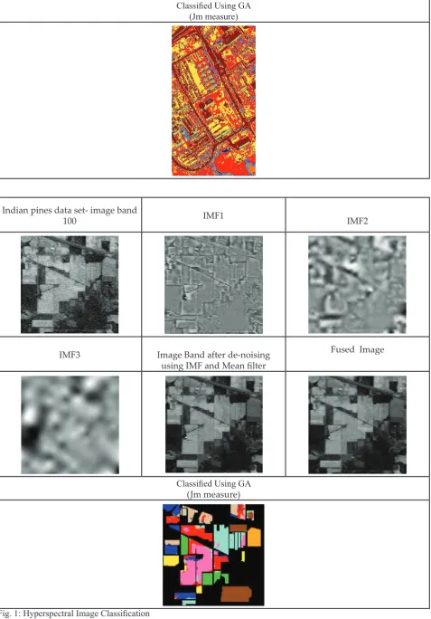
The proposed methodology is tested on Pavia University and Indian pines hyperspectral image data set. The Pavia University data set contains 103 spectral bands and image in each band consists of 610*340 pixels. The Indian Pines data set contains 200 spectral bands and image in each band consists of 145*145 pixels. The data sets are collected from [11] that consist of nine classes in Pavia university data set and sixteen classes in Indian

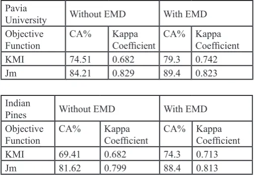
Pines data set with the geometric resolution is 1.3 meters. The experimental result is conducted on band 100 in each of the data set and is shown in fig. 1. The same procedure is executed for all bands in the data set in-order to enhance the image and finally increase the classification accuracy. The bands are selected using SAM measure. The qualitative analysis of the proposed method on Pavia University and Indian Pines hyperspectral data set is shown in fig. 1. Table 1 specifies the quantitative index values of the proposed method compared with the ground truth information available in [11].

Table 1: Classification Accuracy of Proposed Method on Two Different Data Sets

Pavia

University Without EMD With EMD

Objective

Function CA% Kappa Coefficient CA% Kappa Coefficient

KMI 74.51 0.682 79.3 0.742

Jm 84.21 0.829 89.4 0.823

Indian

Pines Without EMD With EMD

Objective

Function CA% Kappa Coefficient CA% Kappa Coefficient

KMI 69.41 0.682 74.3 0.713

Jm 81.62 0.799 88.4 0.813

VII. Conclusion

In this paper, hyperspectral image classification based on EMD and Image fusion is presented. EMD is used in the preprocessing stage for removal of noise in hyperspectral bands. After noise removal, band section technique is used to select the bands that contain valuable information required for classification. The selected image bands are fused into a single image for visualization purpose. This fused image is classified using Genetic algorithm with two different objective functions. The experimental results show that Jm index as objective function in GA classifies the hyperspectral image more efficiently.

References

[1] Yi Ma, Jie Zhang, Yufeng Gao, et.al.,"High Resolution Remote Sensing Image Classification of Coastal Zone and its Automatic Realization”, Proceedings of IEEE International Conference on Computer Science and Software Engineering, pp. 827-829, 2008

[2] Xiaofang Liu,"Remote Sensing Image Classification Using Function Weighted FCM Clustering Algorithm”, Proceedings of IEEE International Geosciences and Remote Sensing Symposium, pp. 2010-2013, 2007.

[3] Nor Ashidi Mat Isa, Samy A.Salamah, Umi Kalthum Ngah,"Adaptive Fuzzy Moving K-means Clustering Algorithm for Image Segmentation”, IEEE Transactions on Consumer Electronics, Vol. 55, Issue 4, pp. 2145-2153, 2012.

[4] Siti Naraini Sulaiman, Nor Ashidi Mat Isa,“Denoising based Clutering Algorithms for Segmentation of Low level of Salt and Pepper Noise Corrupted Images”, IEEE Transactions on Consumer Electronics, Vol. 56, No. 4, November 2010. [5] J. C. Nunes, et.al.,“Image analysis by bidimensional empirical

12, pp. 1019–1026, 2003.

[6] Zeiler A.,et.al.,“Empirical Mode Decomposition- an Introduction”, In Proceedings of IEEE International Joint Conference on Neural Networks, pp. 1-8, 2010.

[7] Alp Erturk, et.al.,"Hyperspectral Image Classification Using Empirical Mode Decomposition with Spectral Gradient enhancement”, IEEE Transactions on GEoscience and RemoteSensing, Vol. 51, No. 5, May 2013, pp. 2787-2790. [8] Ketan Kotwal,et.al.,“Visualization of Hyperspectral Images

Using Bilateral Filtering”, IEEE transactions of Geoscience and remote Sensing, Vol. 48, No. 5, May 2010, pp. 2308-2319.

[9] B. Guo, S. Gunn, B. Damper, J. Nelson,“Hyperspectral image fusion using spectrally weighted kernels,” In Proc. 8th Int. Conf. Inf. Fusion, Philadelphia, PA, Jul. 2005, Vol. 1, pp. 402–408.

[10] J.Harikiran, et al.,"Multiple Feature Fuzzy C-means clustering algorithm for segmentation of microarray image”, Internatonal journal of Electrical and Computer Engineering, Vol. 5, pp. 1045-1053, 2015.

[11] [Online] Available: http://www.ehu.eus/ccwintco/index. php?title=Hyperspectral_Remote_Sensing_Scenes. [12] B.Saichandana, et.al.,"Clustering Algorithm Combined

with Empirical Mode Decomposition for Classification of Remote Sensing Image”, IJSER, Vol. 5, Issue 9, pp. 686-695, 2014.

[13] Subhasis Chaudhuri, Ketan Kotwal,“Hyperspectral Image Fusion”, Springer book.

[14] J.Holland,"Adaptation in Natural and Artificial Systems”. Ann Arbor, MI: Univ. of Michigan Press, 1975.

[15] A.Erturk, et.al.,“Hyper Spectral Image Classification Using Empirical Mode Decomposition with Spectral Gradient enhancement”, IEEE Transactions on Geoscience and Remote Sensing, Vol. 51, Issue 5, pp. 2787-2798.

[16] B.Sanghamitra, et.al.,“Multiobjective Genetic Clustering for Pixel Classification in Remote Sensing Imagery”, IEEE Transactions on Geoscience and Remote Sensing, Vol. 45, No. 5, pp. 1506-1512, 2007.

[17] Yeh Fen, Yang, et.al.,“Genetic Algorithms for Multispectral Image Classification”, [Online] Available: http://www.isprs. org/proceedings/XXXVI/part3/singlepapers/P_16.pdf. [18] J. N. Sweet,“The spectral similarity scale and its application

to the classification of hyperspectral remote sensing data,” In Proc.Workshop Adv. Techn. Anal. Remotely Sensed Data,Washington, DC, Oct. 2003, pp. 92–99.

[19] B. Park, W. R. Windham, K. C. Lawrence, D. P. Smith, “Contaminant classification of poultry hyperspectral imagery using a spectral angle mapper algorithm,” Biosyst. Eng., Vol. 96, No. 3, pp. 323–333, Mar. 2007.

[20] O. A. De Carvalho, P. R. Meneses,“Spectral correlation mapper (SCM): An improvement on the spectral angle mapper (SAM)”, In Proc. Workshop Airborne Geoscience, Pasadena, CA, 2000 [Online]. Available: ftp://geo.arc.nasa.gov/pub/ stevek/Spectral\%20Correlation/ smar_1_carvalho__web. pdf.

Pavia University image band 100 IMF1 IMF2

Classified Using GA (Jm measure)

Indian pines data set- image band

100 IMF1 IMF2

IMF3 Image Band after de-noising

using IMF and Mean filter

Fused Image

Classified Using GA (Jm measure)