Intensity-curvature functional based digital high pass filter of the bivariate cubic B-spline model polynomial function

(1)

O R I G I N A L A R T I C L E

Open Access

Intensity-curvature functional based digital

high pass filter of the bivariate cubic

B-spline model polynomial function

Carlo Ciulla

1*

and Grace Agyapong

2

Abstract

This research addresses the design of intensity-curvature functional (ICF) based digital high pass filter (HPF). ICF is calculated from bivariate cubic B-spline model polynomial function and is called ICF-based HPF. In order to calculate ICF, the model function needs to be second order differentiable and to have non-null classic-curvature calculated at the origin (0, 0) of the pixel coordinate system. The theoretical basis of this research is called intensity-curvature concept. The concept envisions to replace signal intensity with the product between signal intensity and sum of second order partial derivatives of the model function. Extrapolation of the concept in two-dimensions (2D) makes it possible to calculate the ICF of an image. Theoretical treatise is presented to demonstrate the hypothesis that ICF is HPF signal. Empirical evidence then validates the assumption and also extends the comparison between ICF-based HPF and ten different HPFs among which is traditional HPF and particle swarm optimization (PSO) based HPF. Through comparison of image space and k-space magnitude, results indicate that HPFs behave differently. Traditional HPF filtering and ICF-based filtering are superior to PSO-based filtering. Images filtered with traditional HPF are sharper than images filtered with ICF-based filter. The contribution of this research can be summarized as follows: (1) Math description of the constraints that ICF need to obey to in order to function as HPF; (2) Math of ICF-based HPF of bivariate cubic B-spline; (3) Image space comparisons between HPFs; (4) K-space magnitude comparisons between HPFs. This research provides confirmation on the math procedure to use in order to design 2D HPF from a model bivariate polynomial function.

Keywords:Intensity-curvature functional, High pass filter, B-spline, Particle swarm optimization, K-space

Introduction

Recently, we reported a methodology to design digital HPFs from three model polynomial functions. This methodology benefits from the intensity-curvature con-cept and is based on the calculation of the intensity-curvature functional (ICF). The ICF replaces the image intensity value with the product of the image intensity and the sum of second-order partial derivatives of the model function fitted at each pixel. We propose the ICF of the bivariate cubic B-spline model function as a HPF to extend the earlier study [1], and to reinforce the use of the intensity-curvature concept for calculating the

polynomial HPF from a model polynomial function which, in the present study, is the bivariate cubic B-spline. The originality of this study is thus to hypothesize that the ICF of an image is its HPF, and to describe a mathematical model which corroborates, both theoretic-ally and empirictheoretic-ally, that the ICF is indeed a HPF. From the aforementioned mathematical model, it is possible to derive the equations for the input and output functions of the filter. The novel ICF-based filter is compared with the traditional HPF and the PSO-based HPF. A compari-son of the image space and the k-space magnitudes indi-cates that the three filters behave differently. Although the data provided in this study does not allow generalization, traditional HPF filtering and ICF-based filtering are find to be superior to PSO-based filtering. Further, the images filtered with the traditional HPF are sharper than that with the ICF-based filter. The novel

© The Author(s). 2019Open AccessThis article is distributed under the terms of the Creative Commons Attribution 4.0 International License (http://creativecommons.org/licenses/by/4.0/), which permits unrestricted use, distribution, and reproduction in any medium, provided you give appropriate credit to the original author(s) and the source, provide a link to the Creative Commons license, and indicate if changes were made.

* Correspondence:[email protected]

1_{Faculty of Information Systems, Visualization, Multimedia, and Animation,}

University of Information Science and Technology, St. Paul the Apostle, Partizanska B.B., Ohrid 6000, Republic of North Macedonia

(2)

contributions of this study can be summarized as fol-lows: (1) Reasoning to elucidate the mathematical condi-tions that the ICF needs to obey, in order to behave as a HPF; (2) Mathematical description of ICF-based HPF of the bivariate cubic B-spline; (3) Comparison between the image spaces of the three HPFs; (4) Comparison be-tween the k-space magnitudes of the three HPFs.

This section comprises a literature review on HPF and the ICF. The originality of the approach is then dis-cussed in terms of the implications of the mathematical model.

Literature on ICF

HPFs are electronic devices which allow signals with a frequency higher than a particular cutoff frequency, while removing other signals with a frequency lower than the cutoff frequency. The degree of attenuation for each frequency depends on the filter design [2]. The de-sign of digital filter algorithms can be classified into two main categories: finite impulse response (FIR) and infin-ite impulse response (IIR). The FIR filter design is char-acterized by the product of the ideal impulse response with a window function (Butterworth, Chebyshev, Kaiser, and Hamming among others) or a gradient-based optimization method [3–5]. In contrast, the IIR filter de-sign is characterized by a non-zero impulse response function of an infinite time duration [3]. The FIR filters can be optimally designed by a careful selection of coef-ficients for the frequency response, which can be written as a trigonometric function of the frequency [6, 7]. The state-of-the-art design of optimization techniques for implementing FIR digital filters includes the evolutionary and swarm optimization approaches, such as the PSO algorithm [5, 8]. ICF-based digital HPFs have been re-cently realized [1], where they were tested and character-ized using two-dimensional images, and were observed to be belonging to the category of HPFs based on the polynomial functions [9]. The ICF is a property of the model polynomial function which is fitted to the image data on a pixel-by-pixel basis. The essence idea of ICF is to replace the image intensity with the product of the image intensity and the sum of second-order partial de-rivatives of the model polynomial function fitted at each pixel. Since this concept is enforced on a pixel-by-pixel basis, the ICF is an image. The original hypothesis of the above study was that the ICF is a HPF. The rationale of the present study is to revisit the aforementioned hy-pothesis using a new model polynomial function and to validate it through the methodological approach used earlier [1]. The visual appearance of the ICF, which is a high pass (HP) filtered signal, was first observed while investigating the ICF of the bivariate linear model func-tion. Since then, this investigation has been extended to

other model polynomial functions such as bivariate cubic and Lagrange polynomials [1]. In this study, we extend the methodological approach used for the design of a digital HPF to the bivariate cubic B-spline model function. As will be discussed in section 2, the ICF and pixel intensity are set as the output and input functions of the filter, respectively. To evaluate the novel ICF-based HPF, its k-space is compared with that of the trad-itional HPF and the PSO-based HPF.

(3)

Theory

ICF of bivariate cubic B-spline model function

Let us consider the bivariate cubic B-spline model func-tion as defined in eq. (1). This function benefits from 1.

The property of second-order differentiability in its do-main of definition (the pixel) and 2. The non-null classic-curvature of the model function calculated at the origin (0, 0) of the pixel coordinate system [10]. It uses the pixel intensity value f(0, 0) and eight neighbor-ing pixel intensity values: f (1/2, 1/2), f (−1/2, −1/2), f (2/3, 2/3), f (−2/3,−2/3), f (−1,−1), f (1, 1), f (3/2, 3/2) and f (−3/2,−3/2).

h4ðx;yÞ ¼fð0;0Þ þα3 "

1 2

!

ðxþyÞ3₋_ð_x_þ_y_Þ2_þ 2

3

!#

þα2 "

−ð1=6ÞðxþyÞ3þ ðxþyÞ2−2ðxþyÞ þ 4 3

!#

ð1Þ

where:

α2¼ "

fð0;0Þ−f 1 2;

1 2

!#

ð2Þ

α3¼ "

fð0;0Þ−f −1 2;−

1 2

!#

ð3Þ

The first order partial derivatives of h4(x) with respect to the x and y variables are given in eq. (4):

∂ðh4ðx;yÞÞ ∂x

!

¼ ∂ðh4ðx;yÞÞ ∂y

!

¼α3

" 3 2

!

ðxþyÞ2₋₂_ð_x_þ_y_Þ

#

þα2

" − 3

6 !

ðxþyÞ2_þ₂_ð_x_þ_y_Þ₋₂

#

ð4Þ

The second order partial derivatives of h4(x) are given in eq. (5):

∂2ðh4ðx;yÞÞ

∂x2

!

¼ ∂2ðh4ðx;yÞÞ

∂y2

!

∂x∂y

!

∂y∂x

!

¼α3 ½3ðxþyÞ−2 þα2 ½−ðxþyÞ þ2 ð5Þ

Let the intensity-curvature term before interpolation be defined as:

Eo¼Eoðx;yÞ ¼

Z Z

fð0;0Þ (

∂2ðh4ðx;yÞÞ

∂x2

!

þ ∂2ðh4ðx;yÞÞ

∂x∂y

!

∂y∂x

!

∂y2

!)

ð0;0Þ

dxdy

ð6Þ

From eq. (5), it follows that: Table 1Characterization of intensity-curvature functional

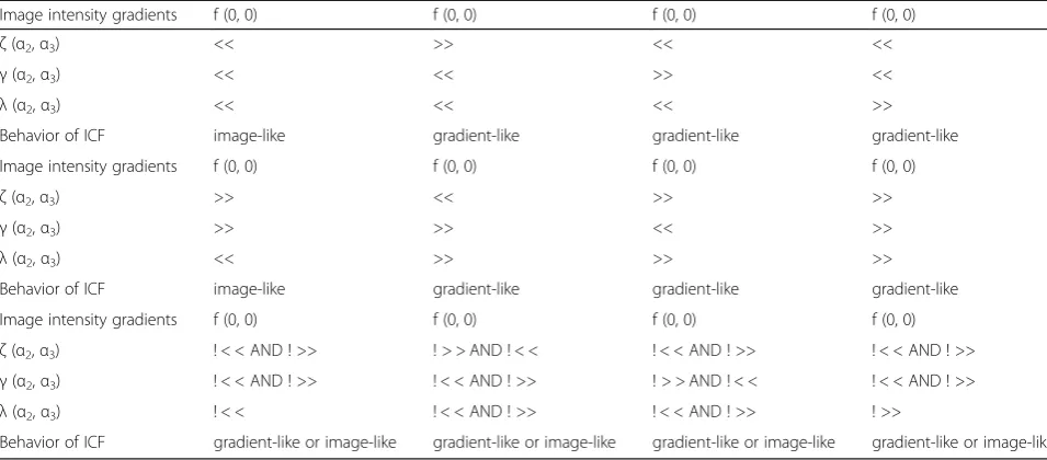
Image intensity gradients f (0, 0) f (0, 0) f (0, 0) f (0, 0)

ζ(α2,α3) << >> << <<

γ(α2,α3) << << >> <<

λ(α2,α3) << << << >>

Behavior of ICF image-like gradient-like gradient-like gradient-like

ζ(α2,α3) >> << >> >>

γ(α2,α3) >> >> << >>

λ(α2,α3) << >> >> >>

Behavior of ICF image-like gradient-like gradient-like gradient-like

ζ(α2,α3) ! < < AND ! >> ! > > AND ! < < ! < < AND ! >> ! < < AND ! >>

γ(α2,α3) ! < < AND ! >> ! < < AND ! >> ! > > AND ! < < ! < < AND ! >>

λ(α2,α3) ! < < ! < < AND ! >> ! < < AND ! >> ! >>

Behavior of ICF gradient-like or image-like gradient-like or image-like gradient-like or image-like gradient-like or image-like

This table can be read by considering: 1. The term in the first column (which isζ(α2,α3) orγ(α2,α3) orλ(α2,α3)); 2. The inequality sign (in the cell of the table); 3.

The value of the pixel intensity f(0, 0). For instance:ζ(α2,α3) < < f(0, 0). The symbols:‘!,’‘<<’,‘>>’,‘AND’; mean different, largely smaller than, largely bigger than,

(4)

∂2ðh4ðx;yÞÞ

∂x2

!

ð0;0Þ

∂y2

!

ð0;0Þ

∂x∂y

!

ð0;0Þ

∂y∂x

!

ð0;0Þ

¼−2α3þ2α2

ð7Þ

Therefore:

Eoðx;yÞ ¼

Z Z

fð0;0Þ n

−2α3þ2α2

o

dxdy¼4xyfð0;0Þ n

−2α3þ2α2

o

ð8Þ

Let the intensity-curvature term after interpolation be defined as:

EIN¼EINðx;yÞ ¼ Z Z

h4ðx;yÞ (

∂2ðh4ðx;yÞÞ

∂x2

!

∂x∂y

!

∂y∂x

!

∂y2

!)

ðx;yÞ

dxdy

ð9Þ

From eq. (5) it follows that:

EINðx;yÞ ¼

Z Z

4h4ðx;yÞ (

α3h3ðxþyÞ−2

i

þα2h−ðxþyÞ þ2 i)

ðx;yÞ

dxdy

¼4 (

fð0;0Þα3 h

3ðx2_y₌₂_þ_xy2₌₂_Þ₋₂_xyi

þfð0;0Þα2 h

−ðx2_y₌₂_þ_xy2₌₂_{Þ þ}₂_xyi)

þ4 ("

3 2α3

2₋1 2α3α2−

3 6α3α2þ

1 6α2

2 #

"

x5_y₌₅_þ3 8x

4_y2_þ_x3_y3₌₃_þ_x2_y4₌₈_þ_x4_y2₌₈_þ_x3_y3₌₃

þ3

8x

2_y4_þ_xy5₌₅ #

þ "

−4α32þ2α3α2þ 4 3α3α2−

4 3α2

2 #

"

x4_y₌₄_þ_x3_y2₌₂_þ_x2_y3₌₂_þ_xy4₌₄ #

þ "

2α32−2α3α2−8α3α2þ4α22 #"

x3_y₌₃_þ_x2_y2₌₂_þ_xy3₌₃ #

þ "

2α32− 2

3α3α2þ8α3α2− 16

3α22 #"

x2_y₌₂_þ_xy2₌₂ #

þ "

−4

3α3 2_þ4

3α3α2− 8 3α3α2þ

8 3α2

2 #

½xy

)

ð10Þ

The ICF of h4(x, y) is defined as:

ΔE xð ;yÞ ¼ E0ðx;yÞ EINðx;yÞ

ð11Þ

Input function x[n] and output function y[n] of ICF-based HPF The TF(x, y) of the ICF-based HPF calculated from the bivariate cubic B-spline is given in eq. (12):

T Fðx;yÞ ¼ Yðx;yÞ Xðx;yÞ

!

¼ ΔEðx;yÞ fð0;0Þ

!

ð12Þ

It implies that:

Yðx;yÞ fð0;0Þ ¼ΔEðx;yÞ Xðx;yÞ ð13Þ

y½n ¼_½ fð0;0Þ e12

4 ðfð0;0Þ α3e1þfð0;0Þ α2e2Þ þω ð

14Þ

Therefore the input function x[n] and the output func-tion y[n] of the ICF-based HPF are:

x½n ¼ ωy½n

½e12−4y½n ðα3e1þα2e2Þ

ð15Þ

y½n ¼ x½n e12

½4 ðx½n α3e1þx½n α2e2Þ þωÞ

ð16Þ

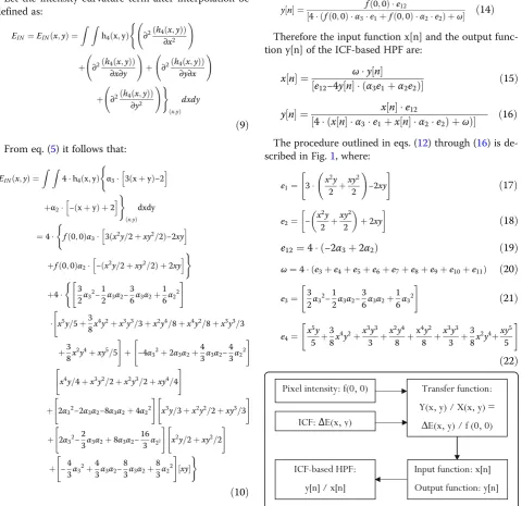
The procedure outlined in eqs. (12) through (16) is de-scribed in Fig.1, where:

e1¼

" 3 x

2_y 2 þ

xy2 2

! −2xy

#

ð17Þ

e2¼ −

x2_y 2 þ

xy2 2

þ2xy

ð18Þ

e12¼4 ð−2α3þ2α2Þ ð19Þ

ω¼4 ðe3þe4þe5þe6þe7þe8þe9þe10þe11Þ ð20Þ

e3¼

" 3 2α3

2₋1 2α3α2−

3 6α3α2þ

1 6α3

2

#

ð21Þ

e4¼

"

x5_y 5 þ

3 8x

4

y2þx

3_y3 3 þ

x2_y4 8 þ

x4_y2 8 þ

x3_y3 3 þ

3 8x

2

y4þxy

5

5 #

ð22Þ

(5)

e5¼ −4α32þ2α3α2þ 4 3 α3α2−

4 3α2

2

ð23Þ

e6¼

x4_y 4 þ

x3_y2 2 þ

x2_y3 2 −

xy4 4

ð24Þ

e7¼ 2α32−2α3α2−8α3α2þ4α22

ð25Þ

e8¼

"

x3_y

3 þ

x2_y2

2 þ

xy3

3

#

ð26Þ

e9¼ 2α32− 2

3 α3α2þ8α3α2− 16

3 α2 2

ð27Þ

e10¼

x2_y 2 þ

xy2 2

ð28Þ

e11¼

" −4

3α3 2_þ4

3α3α2− 8 3α3α2þ

8 3α2

2

#

½xy ð29Þ

Characterization of ICF of bivariate cubic B-spline model polynomial function (H42D)

The behavior of the ICF is highly dependent on the pre-dominance of gradients on the pixel intensity values. Thus, an immediate comparison between the ICF and the image gradients along the X and Y directions indicates that the similarities between the ICF and the HPF may be attributed to the finite differences (gradients) that appear in the for-mulae of ICF and HPF [11]. However, further investigations show that there exists a case where the two intensity curva-ture terms (ICTs) appear similar to the departing image (Fig.2). This happens when the image intensity f(0, 0) pre-vails (both in the numerator and denominator) over the gradient-like components in the ICF formula.

In order to characterize the ICF as a HPF, mathematical formalism is needed so to categorize the ICF as the output function of the equation that defines the transfer function TF of the filter. This mathematical formalism needs to break the ICF formula in components and to analyze each component separately. The mathematical form of the ICF of the bivariate cubic B-spline model polynomial function (H42D) is:

ΔEðx;yÞ ¼4xyfð0;0Þf−2α3þ2α2g=

f4 ffð0;0Þα3 ½3ðx2y=2þxy2=2Þ−2xy

þfð0;0Þα2 ½−ðx2y=2þxy2=2Þ þ2xyg

þ4 f½3 2α3

2₋1 2α3α2−

3 6α3α2þ

1 6α2

2

½x5_y₌₅_þ3 8x

4_y2_þ_x3_y3₌₃_þ_x2_y4₌₈_þ_x4_y2₌₈_þ_x3_y3₌₃

þ3 8x

2_y4_þ_xy5₌₅_{þ ½}₋_4α

32þ2α3α2þ 4 3α3α2−

4 3α2

2

½x4_y₌₄_þ_x3_y2₌₂_þ_x2_y3₌₂_þ_xy4₌₄

þ½2α32−2α3α2−8α3α2þ4α22½x3y=3þx2y2=2þxy3=3

þ½2α32− 2

3α3α2þ8α3α2− 16

3α2

2_½_x2_y₌₂_þ_xy2₌₂

þ½−4

3α3 2_þ4

3α3α2− 8 3α3α2þ

8 3α2

2_½_xy_g

¼ fð0;0Þ e12

f4 ½ðfð0;0Þ α3e1þfð0;0Þ α2e2Þ þωÞg

¼ fð0;0Þ ζðα2;α3Þ ½fð0;0Þ γðα2;α3Þ þλðα2;α3Þ

ð30Þ

In general, as can be deduced from the ratio of eqs. (8) and (10), the ICF can be reduced to the following representation:

(6)

ΔEðx;yÞ ¼ fð0;0Þ ζðα2;α3Þ

½fð0;0Þ γðα2;α3Þ þλðα2;α3Þ

¼₍ ζðα2;α3Þ

γðα2;α3Þ þ

" λðα2;α3Þ

fð0;0Þ #)

ð31Þ

where it is posited that:

ζðα2;α3Þ ¼e12 ð32Þ

γðα2;α3Þ ¼ ½4α3e1þ4α2e2 ð33Þ

λðα2;α3Þ ¼ω ð34Þ

The gradient-like appearance of the ICF is thus deter-mined by the numerical prevalence of the terms that are function of the convolutions (ζ(α2,α3),γ (α2, α3) andλ (α2, α3)). Otherwise, when f(0, 0) prevails, the ICF ap-pears similar to a magnetic resonance image (MRI).

In eq. (31), we assume that ζ(α2, α3) < < f(0, 0) and γ (α2, α3) < < f(0, 0) and λ (α2, α3) < < f(0, 0). In this case, the prevalent term in the numerator and denominator is the image intensity f(0, 0) (this case is illustrated in Fig.2). On the contrary, if we assume thatζ(α2,α3) > > f(0, 0) and

γ(α2,α3) > > f(0, 0) andλ(α2,α3) > > f(0, 0), the prevalent terms areζ(α2, α3) andγ (α2,α3) and the ICF image ap-pears as a HPF. Table 1 indicates that all the remaining cases can be reduced to either of the two listed above.

To summarize, when f(0, 0) is the prevailing term, the ICF reflects the predominant influence of the pixel in-tensity value f(0, 0). On the contrary, when α2 and α3 are both larger than f(0, 0), the ICF behaves as a HPF because of the gradient-like componentsα2andα3.

In essence, the characterization of the ICF as a HPF ac-knowledges that when the convolutions of pixel intensity values in the defining equation of the ICF are tuned as the finite differences operating as gradients, they (the convolu-tions) create the HP filtering effect. This happens under the condition that the convolutions are prevalent on the image

(7)

intensity value. To break the ICF formula into components (as illustrated in eq. (31)) and to build the table, may be ex-tended to other model polynomial functions in order to in-vestigate the effect of gradient-like components and image intensity on the appearance of the ICF image.

Ethics approval and consent

The MRI scans were conducted with the sole purpose of this study and not for clinical purpose. The study partic-ipants were anonymized. Informed consent to participate in the study was obtained from the participants, and this consent allows to publish the MRI images while protect-ing the privacy of the participants.

Results

Comparison between ICF and traditional HP filtering and PSO filtering approaches

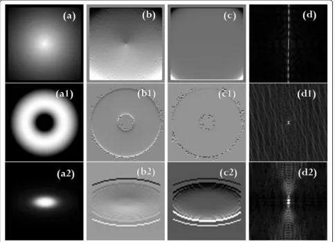
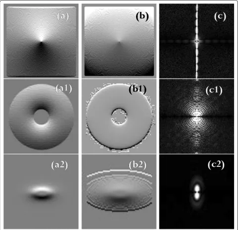
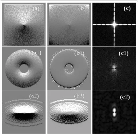
The data set consisted of ten theoretical images and two MRIs. This section illustrates, for the selected cases, the results of filtering with the ICF, the traditional HPF, and the PSO. For the remaining cases, the three filters per-formed in a similar manner. For each of the three filters, the TF and the k-space magnitude of the filtered images is shown in Figs. 3, 4 and 5, respectively. Moreover, to reinforce the difference between the three filters, we show the k-space magnitude images of the filtered images, the difference calculated between the filtered images, and the difference calculated between the k-space images.

It is noteworthy from Figs.3and4that the ICF images are well behaved, however, the HPF images are sharper than the ICF images. The difference between the HPF and ICF images is of particular significance, and it is remark-ably visible in the k-space magnitude [compare Figs.3(d), (d1), (d2) with Figs.4(c), (c1), (c2), respectively].

The images presented in Figs.3,4, and5show the super-iority of the traditional HPF and the ICF-based filter over the PSO-based filter, and this is noticeable if we compare the filtered images in Fig. 4(a), (a1), and (a2) with that in Figs.5(a), (a1), and (a2), respectively. There exist similarities between the k-space magnitude of the HPF filtered images and that of the PSO filtered images (compare Fig.4(c), (c1), and (c2) with Fig.5(c), (c1), and 5(c2), respectively).

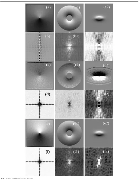
The images displayed in Fig. 6 are a clear and straightforward presentation of the existing differences between the filters discussed in this paper. These im-ages show the difference between the image space and k-space.

Comparison of proposed approach with similar existing methods

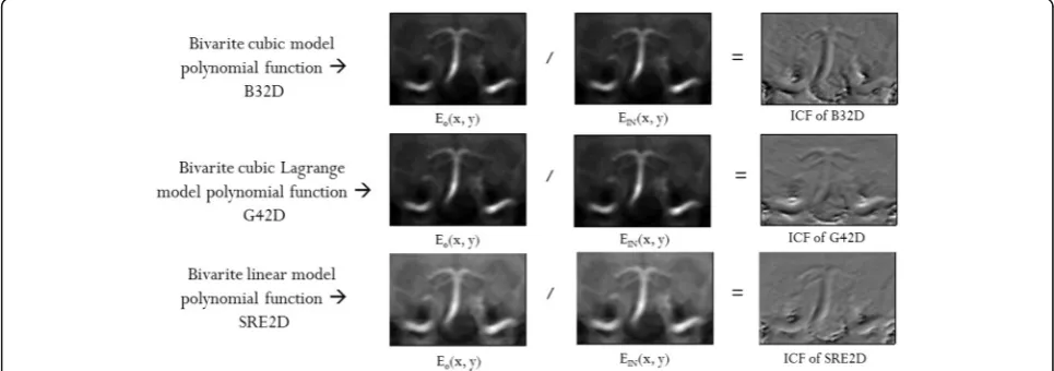
Figure 7 shows a comparison across ICF-based HPFs and the traditional HPF. The model functions and the characterization of the B32D ICF-based HPF and the

G42D ICF-based HPF are reported elsewhere [1]. Through the comparison of the k-space magnitude of the HP filtered images, Fig. 7 clearly shows that these filters are not similar, and their difference can be attrib-uted to the mathematical form of the departing polyno-mial from which the ICF is obtained.

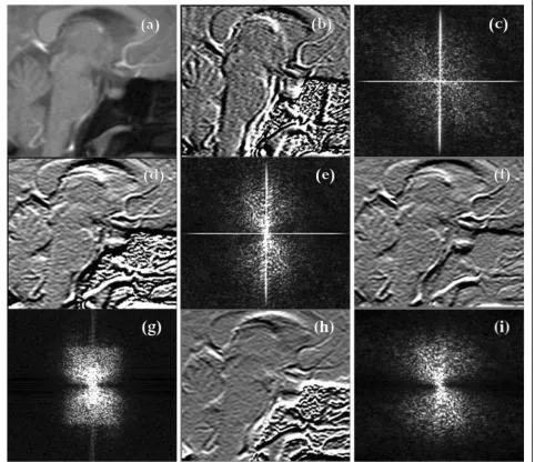
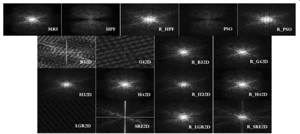
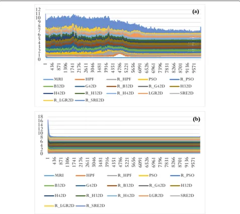
Figures7,8, and9show a comparative study between imaging modalities involving the ICF of several model functions as k-space filters. The MRIs are compared with ICFs, and the ICFs are used as k-space filters through the signal processing technique, known as the inverse Fourier transformation [12]. Figure 8 provides two important aspects of this study. The first aspect is the reproducibility of the HPF behavior of the ICF for six model polynomial functions (including the bivariate cubic B-spline which is the model used in this paper). The other aspect is to verify that the inverse Fourier transformation technique facilitates MRI signal recon-struction. The signal reconstruction highlights the ves-sels of the human brain. Figure 8 also presents the comparison of ICFs with traditional HPF and PSO-based HPF. Figure 9 shows the difference between the k-space of each imaging modality. Through the histo-gram plots of the k-space images, Fig. 10 provides a quantitative outlook of the difference between the fil-tering techniques.

Figures 8 and 9 show the filtered signals and their k-space magnitudes, respectively. Figure 10 shows the re-sults of statistical analysis performed on the filtered im-ages [see (a)] and the k-space magnitude imim-ages [see (b)]. The histogram was calculated for each image, and the cor-responding value of the mean and standard deviation were also computed. The plots in Fig.10show cumulative lines. Each line represents an image and connects the value f(x,

μ,σ) of the normal distribution obtained from each of the

‘x’histogram values. For instance, the histogram value ‘x’ provides the value f(x,μ, σ), which is the integral of the normal distribution from -∞to‘x’, expressed as fðx;μ;σÞ ¼ ð ffiffiffiffiffiffi1

2πσ

p _Þ_e−½ðx−μÞ2=ð2σ2_Þ

. The graphs shown in Figs. 10(a) and (b) are thus cumulative normal distribution values. The plots of f(x,μ,σ) confirm that the filtered signals (Fig. 8) are Gaussian distributed, whereas the k-space signals (Fig.9) are not.

(8)

Discussion

Applications of digital filters literature

The literature on digital filters is extensive. This section provides a compendium of studies corresponding to two most important themes. One theme is related to the ef-fort of the scientific community towards the design of digital filters, with an emphasis on the hardware imple-mentation. The other theme reports on the application of digital filters in academic research and industry set-tings. Table 2 provides a list of authors who have con-tributed to this topic. Study of electroencephalography

(EEG) traces was motivated by the identification of inter-ictal high frequency oscillations (HFOs). This research raised a methodological issue which comes into play when HFOs are filtered because they embed sharp tran-sient frequency components, which result in the so-called confounding false ripples of EEG signal [13] while being filtered. Thus, the identification and quantification of false ripples was pivotal for the correct analysis of broadband activity of various frequency bands. It is also important to determine a strategy that can be used to re-duce the influence of the false ripples on the analysis of

(9)

the EEG signals. Therefore, this study demonstrated that the false ripple occurs during band-pass filtering of the EEG signal, and the false ripple consists of a signal whose frequency is close to the impulse response of the filter, and which appears as a transient signal similar to a short duration oscillation [13]. Another report on appli-cation of digital filters in human technology [14] demon-strated the benefits of filtering out the raw surface empirical mode decomposition (sEMD) signal while esti-mating the muscle forces in the human body. This study found a novel use of the HPFs that can remove up to

90% - 99% of the sEMD signal power, and this can im-prove the force estimates of the specific muscles in the body. Another technological application of high-pass electrical mobility filter (HP-EMF) [15], which is related to the size of nanoparticles in the gaseous media, was also reported. The HP-EMFs have shown a potential to serve as a viable technology for diverse applications ran-ging from the synthesis of nanomaterials to monitoring atmospheric nanoparticles. An industrial application of HPFs, i.e., a methodology for the production of metama-terials, was reported in ref. [16]. The metamaterial

(10)

(11)

explored in this study consisted of engineered subwave-length microstructures, and it exhibited ‘plasmonic’ re-sponse to the electromagnetic waves in the terahertz (THz) range. This property caused the metamaterial to behave as a HPF. The purpose of the study was to dem-onstrate the efficiency of the THz plasmonic HPF which consists of high-aspect-ratio micron-sized wire arrays

that are fabricated by micro-stereo-lithography. This study provided a method to tune the plasma frequency by adjusting the geometric parameters of the metamater-ial [16]. In the context of infrared focal-plane array (IRFPA) technology, the significance of the research re-ported in ref. [17] was to explore the analysis of tem-poral HPFs. A new non-uniformity correction method (See figure on previous page.)

Fig. 6(a), (a1), (a2): Difference between the ICF images (Fig.3) and the traditional HPF images (Fig.4). (b), (b1), (b2): Difference between the k-space magnitude images of ICF (Fig.3) and that of HPF (Fig.4). (c), (c1), (c2): Difference between the image space of ICF (Fig.3) and that of PSO (Fig.5). (d), (d1), (d2): Difference between the k-space magnitude of ICF (Fig. 3) and that of PSO (Fig.5). (e), (e1), (e2): Difference between the image space of HPF (Fig.4) and that of PSO (Fig.5). (f), (f1), (f2): Difference between the k-space magnitude of HPF image (Fig.4) and that of PSO image (Fig.5)

(12)

called bilateral filter based temporal high-pass filter (BFTH) was proposed. The main properties of the HPF developed in this study were convergence speed and ghosting artifacts. Through comparison between algo-rithmic performances, the study demonstrated that the BFTH has the fastest speed of convergence and the most stable error. A study aimed towards designing and implementing computationally efficient two-dimensional FIR digital filters was reported in ref. [18]. The design

procedure was based on frequency domain analysis be-cause the Fourier domain favors the analysis of the inter-polated impulse response. This study demonstrated that, as compared to an equivalent conventional FIR filter, in-terpolated finite impulse response (IFIR) filters require only 1/Lth of the adders and multipliers, while offering 1/Lth noise level and 1/√Lth coefficient sensitivity. The IFIR filter comprised of two components (called FIR sec-tions): one generated the sparse set of impulse response

Fig. 8Comparative study across filtering techniques. Top row (from left to right): MRI, HPF, reconstructed MRI through HPF (R_HPF), PSO-based HPF, and reconstructed MRI through PSO (R_PSO). Second row: ICF of B32D, ICF of G42D, reconstructed MRI through ICF of B32D (R_B32D), and reconstructed MRI through ICF of G42D (R_G42D). Third row from the top: ICF of H32D, ICF of H42D, reconstructed MRI through ICF of H32D (R_H32D), and reconstructed MRI through ICF of H42D (R_H42D). Bottom row: ICF of LGR2D, ICF of SRE2D, reconstructed MRI through ICF of LGR2D (R_LGR2D), and reconstructed MRI through ICF of SRE2D (R_SRE2D)

(13)

Fig. 10Normal distribution values, calculated using the formula fðx;μ;σÞ ¼ ð _{ffiffiffiffiffiffi}1 2πσ

p Þe−½ðx−μÞ2₌_ð₂_σ2_Þ

, for the filtered images presented in Fig.8[see lines in (a)] and for the k-space images presented in Fig.9[see lines in (b)]. The plots show cumulative lines. Each line corresponds to an image, and displays the value of f(x,μ,σ) calculated using the value of‘x’(which is the histogram data of the image)

(14)

(15)

values, and the other executed interpolation. The eigen-filter approach was discussed in ref. [19] as a new method for designing linear-phase FIR filters. This method minimized the quadratic cost function of the error (defined in the passband and stopband of the filter) by calculating the difference between the actual ampli-tude response and the desired response of the filter. It was possible to obtain the equation defining a linear sys-tem from the defining equation of the cost function. The eigenvectors, which are the parameters of the filter, could then be calculated from the definite matrix defin-ing the linear system.

A recent review paper [7] presented an overview of methodological approaches for designing hardware effi-cient finite duration impulse response (FIR) filters. A de-sign method for FIR digital filters, which has gained considerable attention recently, is the multiplier-less fil-ter. This filter is hardware efficient, and is designed with the optimization (minimization) of the multiplier-less operations. It was reported that the hardware efficiency of the multiplier-less filters could be achieved on the basis of various indices which indicate the number of hardware components, such as power-of-two-terms, number of adders, number of multiplier and structural adders, number of flip-flops, and zero-valued filter coef-ficients [7]. The theoretical and the implementation as-pects of FIR and IIR variable digital filters (VDFs) was reported in ref. [20]. These filters exhibited frequency characteristics which could be controlled continuously by tuning some parameters such as the poles and the zeros of the digital filter. Two main highlights of this work were as follows: (1) Computational simplicity of the filter design which only required the calculation of the singular value decomposition of a Hankel matrix. (2) Through the aforementioned calculation, the IIR based VDF was guaranteed to be stable and the frequency re-sponse was conserved. The algorithm reported in ref. [21] focused on the design of FIR filters with powers-of-two coefficients (the 2PFIR filter). The algorithm com-prised of two methods. The first method maintained the existing relationships between the coefficients of the conventional FIR and the 2PFIR filters. This method was called proportional relation-preserve (PRP) method. The second method consisted of an application of the simple symmetric-sharpening (SSS) approach. The SSS method used the PRP method as sub-filter and preserved the transition width. Further, it improved the approximation error of the PRP method. Using the PRP and SSS methods, the feasibility of designing a 2PFIR filter of length (N) greater than 200 was demonstrated.

The research work reported in ref. [5] focused on a linear phase infinite-impulse response filter, which was designed through the nature inspired population-based global optimization algorithm known as Cuckoo Search

(CS) [22]. The main aspect of the study was that the controlling parameter, which quantitatively determined the ripple (and thus the amount of energy) in the desired frequency bands (both stop and pass), was experimen-tally set in such a way that the best performance of the filter could be obtained. The current relevance of the study can be attributed to the fact that it presented a comparative evaluation of three nature inspired optimization methods for FIR filter design, which are (1) the Cuckoo search (CS) [22], (2) the PSO [23], and (3) the artificial bee colony (ABC) [24].

Recent literature

Recent efforts in designing a digital FIR filter can be classified into two groups. The first one utilizes L1-norm based optimization techniques for designing the filter, and the second uses evolutionary approaches which mimic the organizational behavior of living beings, such as the well-known PSO algorithm. The essence of the L1-norm based digital filter design is the formulation of the cost function, the determination of a suitable algo-rithm for its minimization, and the acquisition of the fil-ter equation coefficients [25]. A recent research [26] uses genetic algorithms to solve the optimization prob-lem of the L1-norm based filter design, and compares the filter with a wide array of competing techniques such as the PSO [3, 4, 8] and conventional methods such as the least-squares approach [27], the Kaiser window method [28], and the Parks McClellan algorithm [29].

One of the most compelling and state-of-the-art tech-niques in current digital filter design is the PSO ap-proach. This method is essentially an optimization algorithm, and therefore it suffers from the drawback of obtaining the most suitable cost function, the most suit-able parameters to optimize, and the most suitsuit-able optimization rule. As with every adaptive search, the performance of this optimization algorithm is also af-fected by the initially chosen parameter values, and can be stuck in a local minimum of the cost function (in such a case, the optimization does not progress). Various solutions have been proposed in the literature to pro-mote PSO approach as the state-of-the-art technique [30–33], and these have inspired our implementation of the PSO as a simple, quick, and effective approach. Our approach depends on: (1) a least square function as the cost function of the algorithm, (2) the delta rule as the optimization algorithm and (3) cardinal parameters that were chosen on the basis of experience (particle’s pos-ition, particle’s best position, swarm’s best known pos-ition and particle’s velocity, as explained in Wikipedia).

(16)

algorithm, the particle’s position is updated with the sum of its current value and the value of the particle’s velocity. The initialization of the PSO optimization al-gorithm provides the starting values of the cardinal parameters mentioned earlier [35]. The initialization heuristics set the starting values as random numbers, whose sum is the value of the image intensity. One limitation of our implementation is premature conver-gence [36]. We have chosen to implement the algo-rithm reported in Wikipedia due to its inter-application robustness [37]. This means that the algo-rithm is suitable to be re-engineered with little modi-fication so that it can be applied for optimization problems other than the calculation of HP filtered signal. The flow chart of the procedure is given in Fig. 12. Figure 13 shows the results of the optimization process for one case study.

The difference between the present and the earlier [1] study is that the ICF-based HPF is designed from the bi-variate cubic B-spline here, whereas in ref. [1], the filters were designed from other model polynomial functions. Further, the evaluation method implemented is different, as the ICF-based HPF reported here is compared to the PSO-based HPF. Moreover, we have compared the k-space of three HPFs (ICF-based, traditional HPF, and PSO-based) to ascertain that the filtered images are sig-nificantly different.

Contribution

Since its inception, the ICF has been used to study human brain tumors which are imaged with MRI [38] and human brain vasculature which is also imaged with MRI [39], and to mathematically characterize the input and output func-tions of the ICF-based filters using three different model polynomial functions [1]. The appearance of the ICF image as HPF signal demands an explanation. To this end, the main contribution of this study is the mathematical characterization of the ICF as an alternative HPF.

Moreover, this study provides two essential results. The first one is the reasoning that yields the understanding of the ICF formula. It is observed that the ICF embodies two main components: the image intensity and the gradients. The ICF can thus behave according to the prevalence of one component over the other. The prevalence is obtained when: (1) the numerical value of the image intensity is lar-ger than that of the gradients and in such a case the ICF appears as a departing image; or (2) vice-versa and in such case the ICF appears as HP filtered signal.

The second contribution is the comparison of the ICF-based filter with the traditional HPF and the PSO-ICF-based HPF. The comparison is carried out in both image space and k-space, and it indicates that the three filters behave differently. Although data provided in this paper does not allow generalization, traditional HPF filtering and ICF-based filtering are found to be superior to

(17)

based filtering. Further, the images filtered with the trad-itional HPF are found to be sharper than that with the ICF-based filter.

Conclusion

In order to provide a mathematical formulation for the characterization of the HPF, the theory section of this paper presents the steps undertaken and the benefits obtained from an earlier research [1]. The first step is to include the ICF into the expression of the TF of the filter as the output function [seeΔE(x, y) in eq. (12)]. The sec-ond step consists of including the image pixel intensity as the input function of the TF of the filter [see f(0, 0) in eq. (12)]. The solution of this equation in x[n] (filter in-put) and y[n] (filter outin-put) is outlined in the mathemat-ical procedure, which starts from eq. (13) and ends at eqs. (15) and (16) for x[n] and y[n], respectively. This mathematical formalism allows the ICF to be classified as a HPF. The validity of the formalism, and thus the practical evidence of the fact that the ICF is an alterna-tive HPF, is shown in Figs. 7 and 8. In conclusion, this paper provides a robust mathematical procedure to de-sign a 2D HPF from a model polynomial function.

Acknowledgements

The authors express sincere gratitude to Dr. Dimitar Veljanovski and Dr. Filip A. Risteski because of the availability of the MR images and also to Professor Ustijana Rechkoska Shikoska for the help provided to coordinate the human resources. Dr. Dimitar Veljanovski and Dr. Filip A. Risteski are affiliated with the Department of Radiology, General Hospital 8-mi Septemvri, Boulevard 8th September, Skopje, 1000, Republic of North Macedonia. Professor Ustijana Rechkoska Shikoska is affiliated with the University of Information Science and Technology (UIST), Partizanska BB, Ohrid, 6000, Republic of North Macedonia. The authors also express gratitude to Benjamin Darkwa Nimo whom, at the time of writing this paper, was a student at UIST and whom contributed to the math reported in the theory section. The authors are grateful to the Editor Dr. Xiuxia Song for the treasured suggestions aimed to improve the presentation style of the manuscript. Many thanks also to the anonymous typesetters. This research was developed across the years 2017 through 2019 when the authors were affiliated with UIST.

Authors’contributions

CC is the provider of the technology (computer programs) used for data collection. GA performed the data collection and analysis as relevant to the

data obtained from three of the HPFs compared by this research. Also, GA was helped to write the mathematics of the ICF-based HPF and part of the literature review. CC wrote the paper.

Funding

The authors had no sources of funding for the research reported in this paper.

Availability of data and materials

The datasets used and analyzed during the current study are available from the corresponding author on reasonable request.

Competing interests

The authors declare that they have no competing interests.

Author details

1_{Faculty of Information Systems, Visualization, Multimedia, and Animation,}

University of Information Science and Technology, St. Paul the Apostle, Partizanska B.B., Ohrid 6000, Republic of North Macedonia.2_{Faculty of} Communication Networks and Security, University of Information Science and Technology, St. Paul the Apostle, Partizanska B.B., Ohrid 6000, Republic of North Macedonia.

Received: 29 March 2019 Accepted: 26 June 2019

References

1. Ciulla C, Rechkoska Shikoska U, Veljanovski D, Risteski FA (2018) Intensity-curvature functional-based digital high-pass filters. Int J Imaging Syst Technol 28(1):54–63.https://doi.org/10.1002/ima.22256

2. Saramäki T (1993) Finite impulse response filter design. In: Mitra SK Kaiser JF (ed) handbook for digital signal processing, New York

3. Mondal S, Vasundhara RK, Mandal D, Ghoshal SP (2011) Linear phase high pass FIR filter design using improved particle swarm optimization. WASET, 2011, 60: 1621_–1627

4. Mandal S, Ghoshal SP, Kar R, Mandal D (2012) Design of optimal linear phase FIR high pass filter using craziness based particle swarm optimization technique. Journal of King Saud University - Computer and Information Sciences 24(1):83_–92.https://doi.org/10.1016/j.jksuci.2011.10.007 5. Sharma I, Kuldeep B, Kumar A, Singh VK (2016) Performance of swarm

based optimization techniques for designing digital FIR filter: a comparative study. JESTECH 19(3):1564–1572.https://doi.org/10.1016/j.jestch.2016.05.013 6. Lim YC, Parker SR, Constantinides AG (1982) Finite word length FIR filter

design using integer programming over a discrete coefficient space. IEEE Trans Acoust Speech Signal Process 30(4):661–664.https://doi.org/10.1109/ TASSP.1982.1163925

7. Chandra A, Chattopadhyay S (2016) Design of hardware efficient FIR filter: a review of the state-of-the-art approaches. JESTECH 19(1):212–226.https:// doi.org/10.1016/j.jestch.2015.06.006

8. Eberhart R, Kennedy J (1995) A new optimizer using particle swarm theory. In: the sixth international symposium on micro machine and human science. IEEE, Nagoya, 4-6 October 1995.

PSO-based HP filtered image MR image

Particle’s velocity

Particle’s best position Particle’s position

Swarm's best known position

(18)

9. Jing ZQ (1987) A new method for digital all-pass filter design. IEEE Trans Acoust Speech Signal Process 35(11):1557_–1564.https://doi.org/10.1109/ TASSP.1987.1165067

10. Ciulla C, Risteski FA, Veljanovski D, Rechkoska US, Adomako E, Yahaya F (2015) A compilation on the contribution of the classic-curvature and the intensity-curvature functional to the study of healthy and pathological MRI of the human brain. IJAPR 2(3): 213_–234. DOI:https://doi.org/10.1504/ IJAPR.2015.073852

11. Ciulla C, Rechkoska US, Risteski FA, Veljanovski D (2018) The use of the intensity-curvature functional as k-space filter: Applications in magnetic resonance imaging of the human brain. In: The 1st international conference of applied computer technologies, University of Information Science and Technology“St. Paul the Apostle”, Ohrid, 21–23 June 2018.

12. Ciulla C (2019) Intensity-curvature functional-based filtering in image space and k-space: applications in magnetic resonance imaging of the human brain. High Frequency 2(1):48–60.https://doi.org/10.1002/hf2.10031 13. Bénar CG, Chauvière L, Bartolomei F, Wendling F (2010) Pitfalls of high-pass

filtering for detecting epileptic oscillations: a technical note on "false" ripples. Clin Neurophysiol 121(3):301–310.https://doi.org/10.1016/j.clinph.2009.10.019 14. Potvin JR, Brown SHM (2004) Less is more: high pass filtering, to remove up

to 99% of the surface EMG signal power, improves EMG-based biceps brachii muscle force estimates. J Electromyogr Kines 14(3):389–399.https:// doi.org/10.1016/j.jelekin.2003.10.005

15. Surawski NC, Bezantakos S, Barmpounis K, Dallaston MC, Schmidt-Ott A, Biskos G (2017) A tunable high-pass filter for simple and inexpensive size-segregation of sub-10-nm nanoparticles. Sci Rep 7:45678.https://doi.org/1 0.1038/srep45678

16. Wu DM, Fang N, Sun C, Zhang X, Padilla WJ, Basov DN et al (2003) Terahertz plasmonic high pass filter. Appl Phys Lett 83(1):201–203.https:// doi.org/10.1063/1.1591083

17. Zuo C, Chen Q, Gu G, Qian WX (2011) New temporal high-pass filter nonuniformity correction based on bilateral filter. Opt Rev 18(2):197–202. https://doi.org/10.1007/s10043-011-0042-y

18. Neuvo Y, Dong CY, Mitra SK (1984) Interpolated finite impulse response filters. IEEE Trans Acoust , Speech, Signal Process 32(3):563–570.https://doi. org/10.1109/TASSP.1984.1164348

19. Vaidyanathan P, Nguyen T (1987) Eigenfilters: a new approach to least-squares FIR filter design and applications including Nyquist filters. IEEE Trans Circuits Syst 34(1):11_–23.https://doi.org/10.1109/TCS.1987.1086033 20. Pun CKS, Chan SC, Yeung KS, Ho KL (2002) On the design and

implementation of FIR and IIR digital filters with variable frequency characteristics. IEEE Trans Circuits Syst II 49(11):689_–703.https://doi.org/10.11 09/TCSII.2002.807574

21. Zhao Q, Tadokoro Y (1988) A simple design of FIR filters with powers-of-two coefficients. IEEE Trans Circuits Syst 35(5):566–570.https://doi.org/10.1109/31.1785 22. Yang XS, Deb S (2010) Engineering optimisation by cuckoo search. Int J Math

Mod Numer Optim 1(4):330–343.https://doi.org/10.1504/IJMMNO.2010.035430 23. Ababneh JI, Bataineh MH (2008) Linear phase FIR filter design using particle swarm optimization and genetic algorithms. Digital Signal Processing 18(4): 657–668.https://doi.org/10.1016/j.dsp.2007.05.011

24. Vural RA, Yildirim T, Kadioglu T, Basargan A (2012) Performance evaluation of evolutionary algorithms for optimal filter design. IEEE Trans Evol Computat 16(1):135_–147.https://doi.org/10.1109/TEVC.2011.2112664 25. Aggarwal A, Rawat TK, Kumar M, Upadhyay DK (2015) Optimal design of FIR

high pass filter based on L1 error approximation using real coded genetic algorithm. JESTECH 18(4):594_–602.https://doi.org/10.1016/j.jestch.2015.04.004 26. Aggarwal A, Rawat TK, Kumar M, Upadhyay DK (2018) Design of optimal

band-stop FIR filter usingL1-norm based RCGA. Ain Shams Engineering Journal 9(2):277_–289.

27. Yu WS, Fong IK, Chang KC (1992) An L1 approximation based method for synthesizing FIR filters. IEEE Trans Circuits Syst II 39(8):578–581.https://doi. org/10.1109/82.168951

28. Kaiser J, Schafer R (1980) On the use of the I0-sinh window for spectrum analysis. IEEE Trans Acoust Speech Signal Process 28(1):105–107.https://doi. org/10.1109/TASSP.1980.1163349

29. McClellan J, Parks TW, Rabiner LR (1973) A computer program for designing optimum FIR linear phase digital filters. IEEE Trans Audio Electroacoust 21(6): 506–526.https://doi.org/10.1109/TAU.1973.1162525

30. Fang W, Sun J, Xu WB (2010) A new mutated quantum-behaved particle swarm optimizer for digital IIR filter design. EURASIP J Adv Signal Process 2009(1):367465.https://doi.org/10.1155/2009/367465

31. Vasundhara, Mandal D, Ghoshal SP, Kar R (2013) Digital FIR filter design using hybrid random particle swarm optimization with differential evolution. Int J Comput Int Sys 6(5):911–927.

32. Chang WD (2015) Phase response design of recursive all-pass digital filters using a modified PSO algorithm. Comput Intel Neurosc 2015:8.https://doi. org/10.1155/2015/638068

33. Hu K, Song A, Xia M, Fan Z, Chen X, Zhang R et al (2015) An image filter based on Shearlet transformation and particle swarm optimization algorithm. Math Probl Eng 2015.https://doi.org/10.1155/2015/414561 34. Chopard B, Tomassini M (2018) Particle swarm optimization. In: an introduction

to metaheuristics for optimization. In: Natural computing series. Springer, Cham, pp 97–102.https://doi.org/10.1007/978-3-319-93073-2_6

35. Li X, Ma S (2017) Multiobjective discrete artificial bee colony algorithm for multiobjective permutation flow shop scheduling problem with sequence dependent setup times. IEEE Trans Eng Manag 64(2):149–165.https://doi. org/10.1109/TEM.2016.2645790

36. Li X, Zhang S, Wong K-C (2018) Nature-inspired multiobjective epistasis elucidation from genome-wide association studies. IEEE/ACM Trans Comput Biol and Bioinf, 2018.

37. Wang D, Tan D, Liu L (2018) Particle swarm optimization algorithm: an overview. Soft Comput 22(2):387–408.https://doi.org/10.1007/s00500-016-2474-6 38. Ciulla C, Veljanovski D, Rechkoska Shikoska U, Risteski FA (2015)

Intensity-curvature measurement approaches for the diagnosis of magnetic resonance imaging brain tumors. J Adv Res 6(6):1045–1069.https://doi. org/10.1016/j.jare.2015.01.001

39. Ciulla C, Rechkoska Shikoska U, Veljanovski D, Risteski FA (2018) Intensity-curvature highlight of human brain magnetic resonance imaging vasculature. IJMIC 29(3): 233–243. DOI:https://doi.org/10.1504/IJMIC.2018.091242

Publisher’s Note