Solving DOPF in VSWGs Integrated Power System Using Improved Evolutionary Programming

Solving DOPF in VSWGs Integrated Power

System Using Improved Evolutionary

Programming

Gonggui Chen1,2

1_{College of Electrical and Electronic Engineering, Huazhong University of Science and Technology, Wuhan 430074,}

Hubei Province, China

2_{Dept. of Electrical Engineering, Hubei University for Nationalities, Enshi 445000, Hubei Province, China}

[email protected]

Hangtian Lei1 _{Haibing Fang}2 _{Jian Xu}2

1_{College of Electrical and Electronic Engineering, Huazhong University of Science and Technology, Wuhan 430074,}

Hubei Province, China

2_{Dept. of Electrical Engineering, Hubei University for Nationalities, Enshi 445000, Hubei Province, China}

Abstract—Wind turbine can be divided into two categories:

fixed speed wind generators (FSWGs) and variable speed wind generators (VSWGs) . VSWGs’s bus can be dealt with as PV-bus or PQ-bus in power flow calculation because reactive power compensation can be performed. Dynamic optimal power flow (DOPF) in VSWGs integrated power system is a typical complex multi-constrained non-convex non-linear programming problem when considering the valve-point effect of conventional generators. In this paper, an improved evolutionary programming (IEP) is proposed to solve DOPF in VSWGs integrated power system. In the methodology, the well-known evolutionary programming (EP) is used as a basic level search, which can give a good direction to the optimal global region. Then, a local search (LS) procedure is adopted as a fine tuning to determine the optimal solution. The modified IEEE 30-bus system is used to illustrate the effectiveness of the proposed method compared with those obtained from EP algorithm. In order to verify algorithm effectiveness in more complex power system, IEEE 39-bus system is used test system. It is shown that the proposed method is capable of yielding higher-quality solutions.

Index Terms— wind power generation, variable speed wind

generators, dynamic optimal power flow, improved evolutionary programming

I. INTRODUCTION

Wind energy is the world’s fastest growing renewable energy source. With the increasing levels of wind generator penetration in modern power systems, one of major challenges in the present and coming years is the optimization control, such as optimal power flow including wind farms [1].

Wind turbine can be divided into two categories: fixed speed wind generators (FSWGs) and variable speed wind

generators (VSWGs) . FSWGs are still widely use in power system. The disadvantages of FSWGs are as follows.

When wind speed jump, huge wind force will pass through wind turbine blade, hit wind generator components including the main shaft, gearbox, engines, and so on. FSWGs mean that wind speed fluctuations are directly translated into electromechanical torque variations. This will bring in great mechanical stress and cause high fatigue damages on the components, and may result in swing oscillations between turbine and generator shaft. Also the periodical torque dips because of the tower shadow and shear effect are not damped by speed variations and result in higher flicker. Furthermore, the turbine speed cannot be adjusted with the wind speed to optimise the aerodynamic efficiency and wind energy utilization coefficient.

Compared with FSWGs, VSWGs turbine speed can be adjusted with wind speed. Mechanical stress is reduced, and gust energy can be absorbed by the means of inertia; wind energy utilization coefficient is improved, and reactive power compensation can be performed. So, VSWGs’s bus can be dealt with as PV-bus or PQ-bus in power flow calculation.

In this paper, the problems of dynamic optimal power flow (DOPF) including VSWGs are researched. The expectation model of wind generators' active power outputs is adopted. DOPF is a typical complex multi-constrained non-convex non-linear programming problem in wind power integrated system when considering the valve-point effect of conventional generators. Both lambda-iterative and gradient technique methods in conventional approaches to the problems are calculus-based techniques and require a smooth and convex cost function and strict continuity of the search space.

In the field of global optimization, evolutionary programming (EP) was investigated and proved to be powerful in solving these problems in the last decades. Correspondent author: Gonggui Chen

EP is a stochastic search technique with biological foundations. However, One disadvantage of EP in solving some of the multimodal optimization problems is its slow convergence to a good near-optimum[2, 3, 4].

In this paper, a new improved evolutionary programming (IEP) methodology is proposed for solving DOPF in VSWGs integrated power system; A simple EP [5] is applied as a basic level search, which can give a good direction to the optimal global region, and a local search (LS) procedure [6, 7] is used as a fine tuning to

determine the optimal solution at the final. IEP methodology enhances the computational accuracy and accelerates convergence rate at the later period of the searching by adopting LS operator which is invoked if fitness evaluation improves.

The modified IEEE 30-bus system and IEEE 39-bus system are used to illustrate the effectiveness of the proposed method for solving the established DOPF model in VSWGs integrated power system compared with those obtained from EP algorithm. It is shown that the proposed method is capable of yielding higher-quality solutions.

II. DOPF MODELIN VSWGS INTEGRATED POWER SYSTEM

Due to the random variation of the wind velocities and load demands, it is difficult to research the DOPF in the power system including wind farms. For simplifying this problem, the dividing-stage strategy is adopted in this paper. Wind power generated by wind turbines has intimate relationship with wind speed. Wind speed is converted into power through characteristic curve of a wind turbine. According to the wind velocity forecasting curves and the load forecasting curves in the planning horizon, the expectations of wind generators' power outputs and the load demands at dispatch interval can be calculated.

A. Constraints

Constraints include equality and inequality constraints. The equation constraint is the power flow formulation constraint while inequality constraints including generator power output, ramp rate and bus voltage are as in(1) -(3) . The constraints of real power generation limit and the ramp rate are taken into account as in (1) .

(

)

(

)

,min ,max

max _i , _it _{Ri i}t min _i , _it _Ri gen

P P D T P P P U T

i N

− −

⎧ _{− ∆ ≤ ≤ + ∆}

⎪ ⎨

∈

⎪⎩ .

(1)

,min Gi ,max,

t

Gi Gi gen

Q ≤Q ≤Q i N∈ . (2)

,min t ,max,

i i i

V ≤V ≤V i N∈ . (3) where Pi,min and Pi,max are the maximum and minimum limits of the power generation of unit i, Pit is the real power output of unit i at the tth interval, Pit-1is the real power output of unit i at the t-1th interval; URiis the up-ramp limit of the ith generator (in units of MW/time-period) ,and DRi is the down-ramp limit of the ith

generator (in units of MW/time-period) ;△T is time interval, Ngen is the number of conventional generating units, and N is the number of system buses (excluding slack bus) ; Vit is the voltage magnitude output of bus i at the tth interval; Qt

Gi is the reactive power output of conventional generating unit i at the tth interval; max is the maximum value of the variable, min is the minimum value of the variable.

After calculating the power flow, the state variables, power loss and real power output of the slack bus generator corresponding to the current control variables are available. The real power output of the slack bus generator will be set to the limit if it violates the limit. After handling overlimit of the real power output of the slack bus generator, the system power balance constraints as in(4) must meet, otherwise adding (4) as penalty terms to the objective function to form a generalized objective function. Details of the generalized objective function used in this paper are given in section C.

1

, 1

0 gen

sl N

t t t t t t

i w av ls ld i

P P P P P P

−

=

∆ =

∑

where ∆Pt _{is the unbalance of the real power at the tth} interval,Ngen-1 represents the number of conventional generating units excluding the slack bus, Pslt is the real power output of the slack bus generator after handling its overlimit at the tth interval, Plst is the total power loss at the tth interval, Pldt is the total load expectation at the tth interval, Pt

w,av is the expectation of wind generators’ real power outputs at the tth interval.

B. Objective Function

Due to the fact that wind generation does not consume the fuel, the utility must purchase all the energy produced by wind generating units. Consequently, the objective is to minimize the following total incremental fuel cost function F associated to Ngen dispatchable units for T intervals in the given time horizon, subject to the above-mentioned equality and inequality constraints.

( )

gen

N T

t i t i

F F P

= =

=

∑ ∑

The inclusion of valve-point loading effects makes the modeling of the fuel cost function of the unit more practical. This increases the non-linearity and local optima in the solution space. Also the solution procedure can easily trap in the local optima in the vicinity of optimal value. The fuel cost function of the ith unit F (Pit) with valve-point loadings are represented as follows

( )

,min

sin( ( )

t t t t

i i i i i i i i i i

F P = +a b P +c P +e f P −P . (6)

where ai, bi, and ci are cost coefficients and ei, fiare constants from the valve-point effect of the ith generating unit.

C. Evaluation Function

most of the nonlinear optimization problems, the constraints are considered by generalizing the objective function using penalty terms.

To sum up, the above problems are generalized as follows

{

( )

( )

lim 2

1 1 1

2 lim 2 1 1 ( ) ( ) gen PQ gen N T T t t

i V i i

t i t i N

T T

t t

Q Gi Gi D

t i N t

min F P K V V

K Q Q K P

= = = ∈ = ∈ = + − + + − + ∆

∑∑

∑∑

∑∑

∑

. (7)

where KV, KQ and KD are variable overlimit penalty coefficients, Vit is the voltage magnitude of bus i at the tth interval (excluding the slack bus and PV bus ) ; Qt

Gi is the reactive power output of generator i at the tth interval; Vilim and QGilim denote the violated upper or lower limits.

In this paper, KV, KQ are set to 1, 1 respectively. Because the unbalance of the real power ∆P is hard to meet, an adaptive penalty function to handle penalty coefficient KD is adopted, KD=k k γβα, where k is the algorithm’s current iteration number; β is a relative violated value of the constraints, γ is a multi-stage assignment value, a is the power of the penalty value.

Meanwhile, several experiments have been done in order to obtain the penalty parameters. In this study, if β≤1 then a=1, otherwise a=2. Furthermore, if β≤0.001, then γ=1, else, if β≤0.01 then γ=10, else, if β≤0.1 then γ=30, else, if β≤1 then γ=100, otherwise γ=300.

III. IEP AND IMPLEMENTS

A. Evolutionary Programming

EP is a powerful global optimization technique, has proved itself effective to handle complex optimization problems [2,3,4].EP starts with a population of randomly generated candidate solutions and evolves towards the better solutions over a number of iterations. It uses probabilistic rules to explore the complex search space. Hence, it is more suitable to effectively handle complex optimization problems. The main stages of EP include initialization, mutation, and competition and selection. The generalized mapping procedure of the EP technique is as follows

1) Representation and initialization

For DOPF problem including VSWG, there are T dispatches by Ngen-1 conventional generating units. An

individualarray of control variable arrays is

1 2

1 1 1 1

1 2

2 2 2 2

1 2

1 1 1 1

1 2 P − − − − ⎛ ⎞ ⎜ ⎟ ⎜ ⎟ ⎜ ⎟ = ⎜ ⎟ ⎜ ⎟ ⎜ ⎟ ⎜ ⎟ ⎝ ⎠ t T t T t T

n n n n

t T

n n n n

P P P P

P P P P

P P P P

P P P P

" " " " # # % # % #

" " " "

. (8)

1,2,

P= "g . (9)

where P is individual vector, g is the number of population individuals, Pnt is the real power output of nth

generating unit at the tth interval.

For the complete g population individuals, the candidate solution of each individual is randomly initialized within the feasible range in such a way that it should satisfy the constraint given by (1) .

2) Power flow and fitness calculation

Through the power flow calculation including wind farms, the state variables, power loss and real power output of the slack bus generator corresponding to the current control variables have been able to get. The real power output of the slack bus generator will be set to the limit if it violates the limit. After handling overlimit of the real power output of the slack bus generator, the system power balance constraints as in(4) must meet, otherwise adding (4) as penalty terms to the objective function to form a generalized objective function. In this paper, (7) is used as the fitness or evaluation function. This is a generalized fitness function used to evaluate the fitness of the candidate solution of each individual. Also, record the individual’s position with the global best fitness as gBest, record the current position of each individual as its current pBest. Set the iteration count k=0.

3) Creation of offspring

The value of each decision variable in the individuals of the offspring population is obtained by perturbing the corresponding variable pi,j in the individuals of the parents population according to

, , , ,

' [ ]_{i j i j}[ ] _{i j}[ ] _{i j}(0,1)[ ]

p k = p k +σ k N⋅ k . (10)

where σi,j[k] denotes the corresponding strategy parameter of pi,j[k] and Ni,j(0,1) [k] is a Gaussian random value generated anew at each time of mutation. If the p’

i,j[k] is outside the range, it is fixed to the boundaries.

' '

, ,max ,min

max [ ]

[ ] [ ] ( )

[ ] i

i j k k _FF k_k pj pj

σ =β − . (11)

where Fi[k] denotes the fitness value of the ith individual in the kth generation; Fmax[k] and Fmin[k] denote the maximum and minimum fitness in the kth generation. where β is a scaling factor, which can be tuned during the process of search for optimum. The value of β used here was suggested by [3,4].

4) Selection and Competition

The q-tournament selection scheme is adopted in this paper. Each individual is assigned a score siaccording to

, 1

q i i l

l

s s

=

=

∑

1 , 0 ,

i l il

i l

if F F s

if F F

< ⎧

= ⎨ _>

⎩ . (13)

B. LS Subroutine

EP is a powerful global optimization technique, has proved itself effective to handle complex optimization problems. However, the standard EP convergence rate is very slow [2,3,4]. Consequently, the IEP of blending the standard EP with the following LS is proposed.

The LS procedure is outlined below [6,7].

The initial search point is taken as PG0, PG0 = [xg10xg20, …,xGd0]T and the evaluation function value at PG0 is

F0

gbest . where D is the number of dimension.

Step 1) The initial LS range is selected around PG0 as follows

min ' 0 '

min ( G min)

Y =P + P −P ×β . (14)

max ' ' 0

max ( max G)

Y =P − P −P ×β. (15)

0 max min ' '

max min

( )(1 )

R =Y −Y = P −P −β . (16)

where Ymin _{and Y}max _{are the lower and upper boundaries of} the local search region; β is the local area parameter which is set to 0.4; '

max P and '

min

P are the vectors of decision variables limits; and R0_{is the initial LS range.P}0

Gbest(best search point at the beginning of LS) and Popt (optimum search point) are set to PG0.

Step 2) The NL LS points are randomly generated as follows

1 1 _{( ,1), 1,2, ,}

m m m

n Gbest L

P =P − +R −×rD n= "N . (17) where r(D,1) is a random number vector of length D, whose elements are randomly generated between -1 and 1 in this paper. If any LS point violates the limits, it is forced within the boundaries. NL is the number of LS points which is set to 5.

Step 3) For each LS point, the evaluation function values are calculated. Then the minimum evaluation function among all is taken as Fm

gbest, and the corresponding PG is taken as PmGbest. The optimum values are updated as follows

IF Fm

gbest< Fm-1gbest then Fopt =Fmgbest and Popt = PmGbest Otherwise Fopt=Fm-1gbestand Popt = Pm-1Gbest.

Step 4) The search range is reduced as 1 _{(1 )}

m m

R =R − × −η . (18) where η is the range reduction parameter which is set to 0.05.

Step 5) m=m+1,if maximum iteration for LS is not reached, the iteration count is incremented by one and the above procedure is repeated from step 2,otherwise, Fopt and Popt are taken as the optimum results found by the LS algorithm.

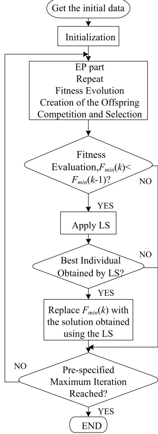
C. IEP and Computational Procedure

The overall procedure of the proposed solution methodology can be summarized as follows

1) Get the initial data;

2) Initialize randomly the initial population in the feasible range and iteration count k=0; Evaluate the initial population and identify the Fmin(0) and the best initial individual;

3) k=k+1,creation of new population by mutation, competition and selection;

4) Evaluate the fitness score for each individual. Identify the Fmin(k) and the best individual of the current iteration k;

5) If Fmin(k) < Fmin(k-1)

6) Solve the DOPF in VSWGs integrated power system using the LS subroutine with the individual of Fmin(k) of the EP as starting point;

7) Replace Fmin(k) of the EP with the final solution obtained using the LS;

8) Repeat for generations until the terminal conditions kmax=150 being satisfied.

So, it is beneficial not only for global optimization in the early evolution but also for the computational accuracy and convergence rate in the later period of the searching.

The above strategies are clearly illustrated in Fig. 1.

END Fitness Evaluation,Fmin(k)<

Fmin(k-1)?

Apply LS YES

NO

Get the initial data

Initialization

EP part Repeat Fitness Evolution Creation of the Offspring Competition and Selection

Pre-specified Maximum Iteration

Reached? Best Individual Obtained by LS?

ReplaceFmin(k) with the solution obtained

using the LS

YES

NO

YES

NO

IV. NUMERICALRESULTS

To verify the effectiveness and efficiency of the adopted IEP for DOPF problems including VSWGs, The modified IEEE 30-bus system (see Fig.2) and IEEE 39-bus system (see Fig.3) are used as the test systems. The procedure has been implemented in Matlab 7.0 programming language and numerical tests are carried on a Pentium 4 2.4G computer. The wind farm including 60 wind generators with the same type, the rating power of which reaches 36MW, are connected to the system at the bus6 for the modified IEEE 30-bus system and at the bus 22 for IEEE 39-bus system respectively. For simplifying the analysis, the load size is considered invariable in the planning horizon. The planning horizon is divided into 9 intervals for the modified IEEE 30-bus system and 12 intervals for IEEE 39-bus system respectively, and every interval is 1hr. The wind generators' outputs are shown in Tab. I for the modified IEEE 30-bus system and Tab. II for IEEE 39-bus system respectively. The modified IEEE 30-bus system data are given in [8]. The modified IEEE 30-bus system parameters of the conventional generating units are shown in Tab. III and Tab. IV [8, 9]. IEEE 39-bus system data are given in[8]. The IEEE 39-bus system parameters of the conventional generating units are shown in Tab. V and Tab. VI [8, 10].

TABLEI

THE WIND FARM DATA IN DIFFERENT PERIODS IN THE MODIFIED IEEE 30-BUS SYSTEM

Stage 1 2 3 4 5 6 7 8 9

Pt w,a

v(MW) 0 4.5 9 13.5 18 22.5 27 31.5 36

TABLEII

THE WIND FARM DATA IN DIFFERENT PERIODS IN THE IEEE39-BUS SYSTEM

Stage 1 2 3 4 5 6 7 8 9 10 11 12

Pt

w,av(MW) 9 12 15 18 36 36 36 36 0 10 14 19

TABLE III

THE PARAMETERS OF CONVENTIONAL GENERATING UNITS IN THE MODIFIED IEEE30-BUS SYSTEM

Generator_($/h) ai _($/MWh) bi _($/MWci 2_{h) (MW/h)} DRi _(MW/h) URi Pi

0 (MW) ei ($/h) fi (rad/MW)

G1 0.0 2.00 0.0200 21.6 21.6 23.54 300 0.2

G2 0.0 1.75 0.0175 18 18 60.97 200 0.22

G22 0.0 1.00 0.0625 14.4 14.4 21.59 150 0.42

G27 0.0 3.25 0.00834 10.8 10.8 26.91 100 0.3

G23 0.0 3.00 0.0250 14.4 14.4 19.2 200 0.35

G13 0.0 3.00 0.0250 18 18 37 200 0.35

TABLE IV

THE LIMITS OF CONVENTIONAL GENERATING UNITS IN THE MODIFIED IEEE30-BUS SYSTEM

Generator Qi,max (MVAr) Qi,min (MVAr) Vi,max (p.u.) Vi,min (p.u.) Pi,max (MW) Pi,min (MW)

G1 150 -20 1.05 0.95 80 0

G2 60 -20 1.05 0.95 80 0

G22 62.5 -15 1.05 0.95 50 0

G27 48.7 -15 1.05 0.95 55 0

G23 40 -10 1.05 0.95 30 0

G13 44.7 -15 1.05 0.95 40 0

G

25 24

15 23 26

21 22 18 19 20 14 13 10 17 16 12 11 9 27 29 30 28 8 6 4 7 3 2

G

G

G

G

G

Fig.2.The modified IEEE 30-bus system

G G G G G G G G G G 30 39 1 2 25 37 29 17 26 9 3 38 16 5 4 18 27 28 36 24 35 22 21 20 34 23 19 33 10 11 13 14 15 8 ₃₁ 12 6 32 7

Fig.3. The39-bus, 10-generator, IEEE system

TABLEV

THE PARAMETERS OF CONVENTIONAL GENERATING UNITS IN THE IEEE 39-BUS SYSTEM

Generator ai ($/h)

bi

($/MWh)

ci

($/MW2_h)

DRi (MW/h) URi (MW/h) Pi0 (MW) ei ($/h) fi (rad/MW)

G30 0.2 0.3 0.01 80 80 250 450 0.041

G31 0.2 0.3 0.01 80 80 572.9 600 0.036

G32 0.2 0.3 0.01 80 80 650 320 0.028

G33 0.2 0.3 0.01 50 50 632 260 0.025

G34 0.2 0.3 0.01 50 50 508 280 0.063

G35 0.2 0.3 0.01 50 50 650 310 0.048

G36 0.2 0.3 0.01 30 30 560 300 0.086

G37 0.2 0.3 0.01 30 30 540 340 0.082

G38 0.2 0.3 0.006 30 30 830 270 0.098

TABLEVI

THE PARAMETERS AND LIMITS OF CONVENTIONAL GENERATING UNITS IN THE IEEE39-BUS SYSTEM

Generator Qi,max (MVAr)

Qi,min

(MVAr)

Vi,max

(p.u.)

Vi,min

(p.u.)

Pi,max

(MW)

Pi,min

(MW)

G30 9999 -9999 1.06 0.94 350 0

G31 9999 -9999 1.06 0.94 1145.55 0

G32 9999 -9999 1.06 0.94 750 0

G33 9999 -9999 1.06 0.94 732 0

G34 9999 -9999 1.06 0.94 608 0

G35 9999 -9999 1.06 0.94 750 0

G36 9999 -9999 1.06 0.94 660 0

G37 9999 -9999 1.06 0.94 640 0

G38 9999 -9999 1.06 0.94 930 0

G39 9999 -9999 1.06 0.94 1100 0

To demonstrate the superiority of the proposed approach for DOPF problems, simulation results have been compared with the EP method. Owing to the randomness in intelligent algorithms, two algorithms are executed 20 times when applied to the test system.

For DOPF problem including VSWGs, Tab. VII and Tab. VIII list the best control variables found by IEP and EP algorithm for the modified IEEE 30-bus system respectively. In Tab. VII, it is clearly shown that, by using IEP, the total production cost savings of 28.3677$/h is obtained compared with EP algorithm. Hence, it is justified that IEP approach gives the exact

minimum dispatch solution. From Tab. XI, the best, worst and average cost values are 9080.5735$/h, 9200.4325$/h, 9132.5035$/h and 9108.9412$/h, 9250.1672$/h, 9188.56373$/h respectively with IEP and EP after 20 independent trials. From the results, the superiority of IEP strategies over EP can be noticed. The difference between the best and worst solutions are 119.859$/h with IEP. At the same time, the difference between the best and worst solutions is 141.226 $/h with EP. Moreover, the best and worst solutions obtained by IEP are very close to the average value, which proves that IEP is more robust and consistent. In conclusion, it is clearly shown that IEP is the most accurate and gives the exact minimum dispatch solution.

In order to verify algorithm effectiveness in more complex power system, IEEE 39-bus system is used test system. Tab. IX and Tab. X list the best control variables found by IEP and EP algorithm respectively. In Tab. IX, it is clearly shown that, by using IEP, the total production cost savings of 815.457$/h is obtained compared with EP algorithm. Hence, The same results are obtained. From Tab. XIII, the best, worst and average cost values are 460571.8601$/h, 461226.8524$/h, 460886.3652$/h and 461387.3171$/h, 462537.4354$/h, 461952.4763$/h respectively with IEP and EP after 20 independent trials. The difference between the best and worst solutions are 654.9923$/h with IEP. At the same time, the difference between the best and worst solutions is 1150.1183 $/h with EP.

TABLEVII

BEST SOLUTION OBTAINED USING IEP METHOD IN THE MODIFIED IEEE30-BUS SYSTEM

Stage 1 2 3 4 5 6 7 8 9

PG1(MW) 32.1628 26.881 30.61201 34.51722 29.78709 31.29296 31.07789 32.61336 16.72349

PG2(MW) 57.00394 61.08434 55.17584 45.11469 52.62017 45.44802 44.2772 43.06717 57.77425

PG22(MW) 23.05492 28.29231 24.03166 30.68287 29.96296 37.48977 29.89494 32.55328 22.52746

PG27(MW) 25.79418 26.01045 30.52419 29.68614 28.98494 30.16027 26.72748 25.80592 20.62617

PG23(MW) 21.3959 18.5878 15.68668 16.15716 9.585935 6.024802 13.87003 15.62889 18.70101

PG13(MW) 32.11083 25.97463 26.30325 21.53214 22.25072 18.29059 18.17907 9.930773 18.55814

Total production cost: 9080.5735 $/h

TABLEVIII

BEST SOLUTION OBTAINED USING EP METHOD IN THE MODIFIED IEEE30-BUS SYSTEM

Stage 1 2 3 4 5 6 7 8 9

PG1(MW) 36.65525 43.1043 30.6769 17.91149 32.04969 15.60642 16.76836 _{13.58982 7.69469}

PG2(MW) 59.36403 58.5255 54.9398 51.61109 56.61143 47.39638 53.91842 _{60.12006 55.17884}

PG22(MW) 21.47479 18.14985 27.65491 30.40768 23.19058 29.44758 29.83708 _{36.22827 30.44646}

PG27(MW) 24.23683 19.73205 20.8879 31.6879 28.29225 31.76615 23.96418 _{21.04326 26.11672}

PG23(MW) 23.43493 17.99541 19.81188 18.72996 15.15849 17.75405 21.13465 _{10.16315 18.56167}

TABLEIX

BEST SOLUTION OBTAINED USING IEP METHOD IN THE IEEE 39-BUS SYSTEM

Stage 1 2 3 4 5 6 7 8 9 10 11 12

PG30(MW) 297.845 306.2852 302.6746 299.8669 274.7264 335.2846 301.1622 294.8944 308.8122 316.6097 302.4517 276.8535

PG31(MW) 550.5877 600.1873 671.5014 605.8921 606.2954 538.8119 564.3921 584.1886 608.1819 607.222 600.5313 586.509

PG32(MW) 626.5221 640.2318 569.7617 622.8446 616.9007 560.5899 594.6618 569.9685 600.4495 646.3009 639.911 624.6706

PG33(MW) 634.3726 610.493 620.8039 614.5901 634.593 653.5109 654.2763 639.7166 623.09 573.336 598.1811 590.8908

PG34(MW) 511.1227 476.2915 443.175 493.175 477.3373 510.5703 460.5703 472.3293 483.933 465.6822 487.3279 491.51

PG35(MW) 610.7836 594.3052 627.8122 590.7639 587.3861 623.3719 618.3914 591.8316 585.7375 566.0117 556.7142 590.8262

PG36MW) 568.042 555.3821 549.7241 570.1911 550.7421 579.9209 586.7932 616.7932 586.7932 587.416 567.623 579.9771

PG37(MW) 527.2084 544.5856 545.6563 542.6359 555.7967 540.9971 550.4644 548.0077 553.644 562.9881 562.9605 539.0908

PG38(MW) 849.1404 850.5165 832.8275 820.6171 850.6171 826.3819 827.0456 840.5518 829.1908 843.1028 819.0072 849.0072

PG39(MW) 1008.702 1001.955 1011.994 1012.711 1002.851 988.7539 999.6285 999.6381 1012.127 1013.031 1042.002 1043.645

Total production cost : 460571.8601 $/h

TABLEX

BEST SOLUTION OBTAINED USING EP METHOD IN THE IEEE 39-BUS SYSTEM

Stage 1 2 3 4 5 6 7 8 9 10 11 12

PG30(MW) 282.7469 238.4208 282.6066 338.1247 341.7531 333.3748 327.2719 306.0325 319.6207 322.2673 342.0072 305.8343

PG31(MW) 594.6711 538.4092 504.6806 435.1558 475.9911 527.6847 564.3274 544.4797 607.5929 661.6504 646.2157 598.6778

PG32(MW) 660.1812 689.5568 631.677 657.2323 622.9245 609.8651 565.3495 554.2467 531.8468 509.444 493.9961 502.6156

PG33(MW) 633.0862 647.1537 657.152 695.4439 656.121 613.5017 634.5771 624.303 650.9625 654.4778 639.7837 643.3003

PG34(MW) 497.4557 495.9905 523.4377 506.0668 491.8216 456.7792 470.8762 449.5858 423.7924 451.8563 445.8726 460.6822

PG35(MW) 605.0152 616.4778 602.7038 583.1142 612.878 641.2923 592.1213 642.1213 650.9918 608.5196 650.9933 665.4863

PG36MW) 544.6999 547.3016 570.5253 579.3933 565.1149 593.0327 567.4237 569.0068 574.9087 564.7232 548.5948 554.9131

PG37(MW) 546.2254 571.3317 582.452 561.9026 563.9268 545.5942 575.5942 574.6134 573.9448 547.9221 550.402 529.3439

PG38(MW) 817.0216 835.4741 852.515 841.1737 846.6516 871.43 864.4906 894.4906 880.61 898.6867 872.7176 902.7176

PG39(MW) 1001.559 1002.257 974.3036 980.9517 982.4731 966.97 996.97 1002.012 981.4998 965.9979 989.3619 1013.062 Total production cost: 461387.3171 $/h

The average execution time taken to complete the fixed number of iterations (Tfix) and the average execution time taken to converge into the lower solution range ( Tlow) for 20 trials are shown in Tab. XII for the modified IEEE 30-bus system and Tab. XIV for IEEE 39-bus system respectively.

For the modified IEEE 30-bus system, EP takes an average execution time of 1800.23 sec. to complete 150 iterations. EP converges faster than IEP by reason of the small sub-memeplex generation number of IEP. In comparison to EP, IEP has additional components, i.e., the LS procedure. This extra burdens increase the execution time of IEP. IEP takes 1898.34 sec. more than EP to complete 150 iterations. Nevertheless, IEP takes only 1020.33 sec. to converge into the lower solution range (9080–9098$/h) , EP are not able to converge into the lower solution range.

For IEEE 39-bus system, EP takes an average execution time of 4247.25 sec. to complete 150 iterations. EP converges faster than IEP by reason of the small sub-memeplex generation number of IEP. In comparison to EP, IEP has additional components, i.e., the LS procedure. This extra burdens increase the execution time of IEP. IEP takes 4347.92 sec. more than EP to complete 150 iterations. Nevertheless, IEP takes only 2243.82 sec. to converge into the lower solution range (460571–

460671$/h) , EP are not able to converge into the lower solution range.

TABLE XI

COMPARISON OF BEST, WORST AND AVERAGE COST VALUES IN THE MODIFIED IEEE30-BUS SYSTEM

Algorithms Best ($/h) Worst ($/h) Average ($/h) IEP 9080.5735 9200.4325 9132.5035

EP 9108.9412 9250.1672 9188.5637

TABLEXII

AVERAGEEXECUTIONTIMECOMPARISON IN THE MODIFIED IEEE30-BUS SYSTEM

Methods Average execution time (sec.) _{Tfix Tlow}

EP 1800.23 ——

IEP 1898.34 1020.33

TABLE XIII

COMPARISON OF BEST, WORST AND AVERAGE COST VALUES IN THE IEEE 39-BUS SYSTEM

Algorithms Best ($/h) Worst ($/h) Average ($/h) IEP 460571.860 461226.8524 460886.365

TABLEXIV

AVERAGEEXECUTIONTIMECOMPARISON IN THE IEEE 39-BUS SYSTEM

Methods Average execution time (sec.) _{Tfix Tlow}

EP 4247.25 ——

IEP 4347.92 2243.82

V. CONCLUSION

Considering the valve-point effect and ramp rate limits of conventional generators including VSWGs, DOPF model, which takes the all conventional units cost minimum as the objective function and takes the whole time and the inherent relations of different stages into account in wind power integrated system, is established. The PV-bus model of VSWGs bus is adopted in power flow calculation in this paper. A novel IEP is proposed for solving the established DOPF model and the detailed methods of the algorithm are given. The modified IEEE 30-bus system is used to illustrate the effectiveness of the proposed method compared with those obtained from EP algorithm. In order to verify algorithm effectiveness in more complex power system, IEEE 39-bus system is used test system. It is shown that the proposed method is capable of yielding higher-quality solutions.

ACKNOWLEDGMENTS

The authors would like to thank anonymous reviewers. This work is supported by the Science Research Program of Education Bureau of Hubei Province under Grant No. D20092906.

REFERENCES

[1] H. Li and z. Chen, “Overview of different wind generator systems and their comparisons,” IET Renewable Power Generation, vol. 2,no.2, pp. 123-138,2008.

[2] X. Yao, y. Liu and G. Lin, “Evolutionary programming made faster,” IEEE Trans. Evol. Comput., vol 3, no. 2, pp. 82-102, 1999.

[3] C. H. Liang, C. Y. Chung, and k. P. Wong etc., “Comparison and improvement of evolutionary programming techniques for power system optimal reactive power flow,” IEE Proceedings-Generation, Transmission & Distribution, vol.153, no.2, pp.228-235, 2006.

[4] J. T. Ma and L. L. Lai, “Evolutionary programming approach to reactive power planning,” IEE Proceedings-Generation, Transmission & Distribution,vol.143, no.4, pp.365-370, 1996.

[5] D. B. Fogel, “An introduction to simulated evolutionary optimization,” IEEE Trans. Neural Networks, vol. 5, no.1, pp. 3–14, 1994

[6] R. Luss and T. H. I. Jaakola, “Optimization by direct search and systematic reduction of the size of the search region,” AICHE J., vol.19, no.4, pp.760–766, 1973. A. I. Selvakumar and K. Thanushkodi, “A new particle

swarm optimization solution to nonconvex economic dispatch problems,” IEEE Transactions on Power Systems,vol.22, no.1, pp.42-51, 2007.

[7] R. D. Zimmierman, C. E. M. Sanchez, and D. Gan :Matpower. a matlab power system simulation package. [online].available:

http://www.pserc.cornell.edu/matpower.

[8] R. Yokoyama, S.H. Bae, T.Morita, H. Sasaki, “Multi-objective optimal generation dispatch based on probability security criteria,” IEEE Transactions on Power Systems, vol. 3,no. 1, pp. 317–324, 1988.

[9] T. A. A. Victoire and A. E. Jeyakumar, “A modified hybrid ep–sqp approach for dynamic dispatch with valve-point effect,” International Journal of Electrical Power And Energy Systems, vol. 27,no. 8, pp. 594–601, 2005.

Gonggui Chen was born in Hubei, China in 1964. He