A Study on Various Types of Beamforming
Algorithms
Saiju Lukose Prof. M. Mathurakani
M. Tech Student (VLSI & Embedded Systems) Assistant Professor
Department of Electronics & Communication Engineering Department of Electronics & Communication Engineering Toc-H Institute of Science and Technology, Toc-H Institute of Science and Technology,
Arakunnam, Kerala, India Arakunnam, Kerala, India
Abstract
This paper deals with the study of various types of Beamforming algorithms. A beam former is a processor used in conjunction with an array of sensors to provide a versatile form of spatial filtering. The sensor array collects spatial samples of propagating wave fields, which are processed by the beam former. The objective is to estimate the signal arriving from a desired direction in the presence of noise and interfering signals. A beam former performs spatial filtering to separate signals that have over lapping frequency content but originate from different spatial locations.
Keywords: Beamforming, Conventional Beamforming, Capon Beamforming, Adaptive, LMS
________________________________________________________________________________________________________
I. INTRODUCTION
Beamforming is the combination of radio signals from a set of small non-directional antennas to simulate a large directional antenna. The simulated antenna can be pointed electronically, although the antenna does not physically move. There are many terrestrial radar applications using beamforming such as mining, weather monitoring where a weather radar can determine the rain locations with a resolution of several hundreds of meters, it is also used to identify the range, altitude, direction, or speed of moving and fixed targets such as aircraft, ships, motor vehicles. In the case of mining as it progresses and monitoring different sections of the pit walls becomes necessary, relocating monitoring devices is not only costly and time consuming, but can also be dangerous on unstable slopes. So a beamforming that can be software controllable is used, here arrival angle of a signal source can be found by steering beam formed antenna and also it minimize the contributions of strong interferers from unknown directions while passing the desired signal from a chosen look direction. When we combine signal from multiple antennas it automatically boosts the signal-to-noise ratio compared to a single antenna. In beamforming, both amplitude and phase of each antenna element are controlled.
Combined amplitude and phase control can be used to adjust side lobe levels and steer nulls better than can be achieved by phase control alone. The combined relative amplitude ak and phase shift qk for each antenna is called a “complex weight” and is represented by a complex constant wk (for the kth antenna). A beamformer for a radio transmitter applies the complex weight to the transmit signal (shifts the phase and sets the amplitude) for each element of the antenna array. In beamforming, both amplitude and phase of each antenna element are controlled. Combined amplitude and phase control can be used to adjust side lobe levels and steer nulls better than can be achieved by phase control alone. The combined relative amplitude ak and phase shift qk for each antenna is called a “complex weight” and is represented by a complex constant wk (for the kth antenna). A beamformer for a radio transmitter applies the complex weight to the transmit signal (shifts the phase and sets the amplitude) for each element of the antenna array. The rest of the paper is organized as follows Section II studies Classical Beamforming, Section III studies Statistically Optimum Beamforming, Section IV deals with Adaptive Beamforming.
II. CONVENTIONAL DOA ESTIMATION METHOD/ BARTLETT METHOD
The Conventional Beamforming Method (CBF) is also referred to as the delay-and-sum method or Bartlett method. The idea is to scan across the angular region of interest (usually in discrete steps), and whichever direction produces the largest output power is the estimate of the desired signal’s direction. More specifically, a s the look direction θ is varied incrementally across the space of access, the array response vector a (θ) and received signal auto covariance matrix Rxx are calculated and the output power of the beamformer is measured by
III. CAPON’S MINIMUM VARIANCE METHOD
The Capon’s minimum variance method is also known as the Minimum Variance Distortion less Look (MVDL). The MVDL is an attempt to overcome the poor resolution problem associated with the delay-and-sum method and it results a significant improvement. In this method, the output power is minimized with the constraint that the gain in the desired direction remains unity. Solving this constraint optimization problem for the weight vector we obtain
This gives the Capon’s Spatial Spectrum
The MVDL only requires an additional matrix inversion compared to the CBF and exhibits greater resolution in most cases. Computing the spatial power spectrum for one range of θ does not prevent the algorithm from subsequently computing the spectrum for another range of θ using the same data. The spatial characteristics of the data for all directions are compactly represented by Rxx, and they are needed to be computed only once. Thus, the method does not have blind spots in time during which transient signals, away from directions of constantly transmitting sources, can appear intermittently and fail to be detected. Another advantage is that by steering the antenna electronically rather than mechanically, the speed of the scan through a region of interest is limited by computational speed instead of mechanical speed.
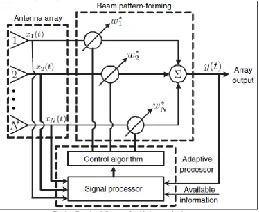
IV. ADAPTIVE BEAMFORMING
For time-varying signal environments, such as wireless cellular communication systems, statistics change with time as the target and interferers move around. For the time-varying signal propagation environment, a recursive update of the weight vector is needed to track a moving interference so that the spatial filtering beam will adaptively steer to the target time-varying DOA, thus resulting in optimal transmission/reception of the desired signal. To solve the problem of time-varying statistics, weight vectors are typically determined by adaptive algorithms which adapt to the changing environment
Fig. 2.1: Functional diagram of an N-element adaptive array
transient-array weights have reached their steady-state values in a stationary environment or are being adjusted in response to alterations in the signal environment. If we consider that the reference signal for the adaptive algorithm is obtained by temporal reference, a priori known at the receiver during the actual data transmission, we can either continue to update the weights adaptively via a decision directed feedback or use those obtained at the end of the training period. Several adaptive algorithms can be used such that the weight vector adapts to the time-varying environment at each sample; among which LMS can is explained below.
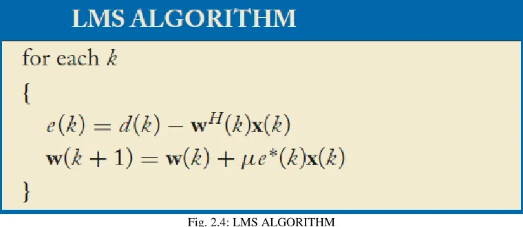
The LMS Algorithm
The LMS algorithm is probably the most widely used adaptive filtering algorithm, being employed in several communication systems. It has gained popularity due to its low computational complexity and proven robustness. It incorporates new observations and iteratively minimizes linearly the mean-square error. The LMS algorithm changes the weight vector w along the direction of the estimated gradient based on the negative steepest descent method. By the quadratic characteristics of the mean square-error function E {|e (k)|^2} that has only one minimum, the steepest descent is guaranteed to converge
Fig. 2.4: LMS ALGORITHM
The LMS algorithm is a member of a family of stochastic gradient algorithms since the instantaneous estimate of the gradient vector is a random vector that depends on the input datavector x(k) . It requires about 2N complex multiplications per iteration, where N is the number of weights (elements) used in the adaptive array. The convergence characteristics of the LMS depend directly on the eigen structure of Rxx . Its convergence can be slow if the eigenvalues are widely spread.When the covariance matrix eigen values differ substantially, the algorithm convergence time can be exceedingly long and highly data dependent. Therefore, depending on the eigenvalue spread, the LMS algorithm may not have sufficient iteration time for the weight vector to converge to the statistically optimum solution and adaptation in real time to the time-varying environment will not be able to be performed . In addition, employing the LMS algorithm, it is assumed that sufficient knowledge of the desired signal is known so as to generate reference signal sequences.
V. RESULT AND DISCUSSION
MATLAB is the simulator used to simulate the beam foming techniques. Firstly, we have done simulations to understand the beamforming. Then we have done the simulations of conventional DOA estimation, Conventional beam former & capon beam formers, and adaptive beam former and the performance is analyzed.
Simulation Parameters:
- Number of antennas : 32 - Distance between adjacent antennas: λ/2 - Signal Magnitude : 10
Conventional Beamforming
Fig. 5.1: Beam pattern plot for conventional Beam forming with desired signal at 40 degrees.
Capon Beamformer
For a uniform linear array with 32 number of antennas, inter-element spacing (d) = 0.5λ , the plot of Beampattern vs array look angle for a single source for capon beamforming is shown in figure 7.5 here our desired signal direction is at 40 degrees and interference at 60 degrees. Desired signal direction=40degrees, Interference direction=60 degrees, Signal Power=1dB, Noise Power=5dB, Interference power=1000dB.
Fig. 5.2: Beampattern plot for Capon Beamforming with desired signal at 40 degrees and interference at 60 degrees.
Adaptive Beamforming
For a uniform linear array with 32 number of antennas, inter-element spacing (d) = 0.5λ , the plot of Beampattern vs array look angle for a single source for Adaptive Beamforming with interferences at directions at 11 degrees and source at 0 degrees.Here the interference signal magnitude is & times the signal power.Here we have simulated it with the help of Generalized Side Lobe Canceller Structure.
Fig. 5.4: Input desired signal, Input Interference Signal, Real Input Received at Beam former
Fig. 5.5: Output from the Conventional Beamformer
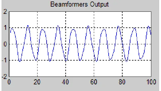
Fig. 5.6: Output from the Adaptive Beamformer in which LMS algorithm is used for correction.
VI. CONCLUSION
REFERENCES
[1] Barry D Van Veen and Kevin M Buckley “Beamforming: A Versatile Approach to spatial filtering” IEEE ASSP MAGAZINE ,Vol 1,1988.
[2] LAL C. GODARA” Application of Antenna Arrays to Mobile Communications, Part II: Beam-Forming and Direction-of-Arrival Considerations”, PROCEEDINGS OF THE IEEE, VOL. 85, NO. 8, AUGUST 1997
[3] Peter Vouras and Brian Freburger “Application of Adaptive Beamforming Techniques to HF Radar”, Radar Conference,Vol 1,No 2,2008 .
[4] Vera Behar, Christo Kabakchiev “Multiple Signal Extraction in Jamming Using Adaptive Beamforming with Arbitrary Array Configurations”, CYBERNETICS AND INFORMATION TECHNOLOGIES, Volume 9, No 3,2010.
[5] Rana Liaqat Ali,Anum Ali,Anis-ur-Rehman ,Shahid A. Khan and Shahzad A. Malik “Adaptive Beamforming Algorithms for Anti-Jamming”,International Journal of Signal Processing, Image Processing and Pattern Recognition ,Vol. 4, No. 1, March 2011.
[6] Asit Kumar Subudhi, Biswajit Mishra , Mihir Narayan Mohanty “VLSI Design and Implementation for Adaptive Filter using LMS Algorithm”, International Journal of Computer & Communication Technology (IJCCT), Volume-2, Issue-VI, 2011.
[7] Balasem. S.S and S.K.Tiong, S. P. Koh “Beamforming Algorithms Technique by Using MVDR and LCMV” ,World Applied Programming, Vol (2), Issue (5), May 2012.
[8] Dhusar Kumar Mondal “Studies of Different Direction of Arrival (DOA) Estimation Algorithm for Smart Antenna in Wireless Communication” ,IJECT, Vol 4, Issue Spl 1, Jan - March 2013.
[9] Arathy Reghu kumar, K. P Soman, Shanmuga Sundaram G.A “Beamforming Algorithm Implementation using FPGA”, ISSN (Print): 2278-8948, Volume-2, Issue-3, 2013.
[10] AMARA PRAKASA RAO and N.V.S.N. SARMA “Adaptive Beamforming Algorithms for Smart Antenna Systems” WSEAS TRANSACTIONS on COMMUNICATIONS, Volume 13, 2014.
[11] Somnath Patra , Abhisek Pandey, Nisha Nandni and Sujeet Kumar “Power pattern synthesis of smart antenna array using different adaptive algorithms” ,International Journal of Advanced Research,Volume 3,2015 .