Artificial Neural Network Models For Software Effort Estimation

Artificial Neural Network Models For Software

Effort Estimation

P.Subitsha, J.Kowski Rajan

(M.E. Student in Applied Electronics ) Department of Electronics and Communication Engineering, Loyola Institute of Technolo-gy & Science, Thovalai, Kanyakumari, India; 2(Assistant Professor) Department of Electronics and Communication Engineering, Loyola Institute of Technology & Science, Thovalai, Kanyakumari, India.

Email: [email protected], [email protected].

ABSTRACT: Software estimation accuracy is one of the greatest challenges for software developers. Software cost and time estimation supports the planning and tracking of software projects. The present paper is directed to design a model which should be accurate and comprehensible in order to inspire confidence in a business setting. Software effort estimation models which adopt a neural network technique provide a solution to improve the accuracy. However, no univocal conclusion to which technique is the most suited has been reached. This study addresses this issue by reporting on the results of a large scale benchmarking study. Different types of techniques are under consideration including techniques such as Multilayered Perceptron Network, Radial Basis Function Neural Network, Support Vector Machines, Extreme Learning Machines and Particle Swarp Optimization. Studies are made using COCOMO II data. Results are provided for MMRE and PRED (25) accuracy measures.

Keywords :Artificial neural network, Cocomo

1 INTRODUCTION

Software cost estimation is the process of predicting the effort required to develop a software system. Many estimation mod-els have been proposed over the last 30 years. In recent years, computing power has become a subordinate resource for software developing companies as it doubles approximate-ly every 18 months, hereby costing onapproximate-ly a fraction compared to the late 60’s. Personnel costs are however still an important expense in the budget of software developing companies. In light of this observation, proper planning of personnel effort is a key aspect for these companies. Software community has developed unique tools and techniques such as size, effort, and cost estimation techniques and tools to address chal-lenges facing the management of software development projects [1][2][3]. These tools and techniques are utilized for software development phases starting with the software re-quirements specification. As demand for software applications increases continually and the software scope & complexity become higher than ever, the software companies are in real need of accurate estimates of the project under development. Indeed, good software effort estimates are critical to both companies and clients. There are several methods available to estimate the cost required to develop software. Each has its own strengths and weaknesses. A major hurdle in software cost estimation is the unavailability of data at the starting time of the project. A key factor in selecting a cost estimation model is the accuracy of its estimates. Unfortunately, despite the large body of experience with estimation models, the accuracy of these models is not satisfactory. Also, from a comprehensi-bility point of view, a more concise model (i.e. a model with less input) is preferred. In this paper, five techniques representing artificial neural network models are investigated. It includes Multi Layered Perceptron (MLP) Neural network, Radial Basis Function (RBF) network, Support Vector Ma-chines(SVM), Particle-Swarm Optimization in SVM (PSO-SVM) and Extreme learning Machines.

2

M

In this research, the Cocomo model (Constructive Cost Mod-el) has been used for the experimentation purposes. It is an algorithmic software cost estimation model developed by Barry Boehm. The model uses a basic regression formula, with

pa-rameters that are derived from historical project data and cur-rent project characteristics. The effort estimation process is done in six phases: Data preprocessing, Technique setup, In-put selection, Evaluation criteria and testing. All these models were trained with first 2/3 inputs from the standard dataset and later 1/3 inputs from the same dataset were used to test the models. Finally a comparative analysis was carried out based on the standard assessment criterions MMRE and Pred (25).

3 TECHNIQUES

As mentioned in Section I, different techniques have been applied to the field of software effort estimation. As the aim of the study is to assess which data mining techniques perform best to estimate software effort, the following techniques are considered 1. These techniques were selected as their use has previously been illustrated in the domain of software effort prediction and/or promising results were obtained in other regression contexts. Computational cost was also taken into consideration in selecting the techniques eliminating tech-niques characterized by high computational loads.

1 The techniques are implemented in Matlab.

MLP: Neural networks (NNs) are a non-linear modeling tech-nique inspired by the functioning of the human brain [4]–[6] and have previously been applied in the context of software effort estimation [7], [8], [9]. We further discuss Multi Layered Perceptrons (MLPs) which are the most commonly used type of NNs that are based upon a network of neurons arranged in an input layer, one or more hidden layers, and an output layer in a strictly feedforward manner. Each neuron processes its inputs and generates one output value via a transfer function, which is transmitted to the neurons in the subsequent layer. The output of hidden neuron i is computedby processing the weighted inputs and its bias term bias follows:

hi = f

z = f

with nh the number of hidden neurons and v the weight vector, whereby v_j represents the weight connecting hidden unit j to the output neuron. The bias term has a similar role as the in-tercept in regression. MLP neural networks with one hidden layer are universal approximators, able to approximate any continuous function [10]. Therefore in this study, a MLP with one hidden layer was implemented. The network weights W and v are trained with the algorithm of Levenberg–Marquardt [11]. In the hidden layer, a log sigmoid transfer function has been used, while in the output layer a linear transfer function is applied. The topology of the neural network is adjusted during training to better reflect specific data sets.

RBFN: Radial Basis Function Networks (RBFN) are a special case of artificial neural networks, rooted in the idea of biologi-cal receptive fields [12]. A RBFN is a three-layer feed- forward network consisting of an input layer, a hidden layertypically containing multiple neurons with radial symmetric gaussian transfer functions and a linear output layer. Due to the conti-nuous target, a special type of RBFN is used, called Genera-lized Regression Neural Networks [13]. Within such networks, the hidden layer contains a single neuron for each input sam-ple presented to the algorithm during training. The output of the hidden units is calculated by a radial symmetric gaussian transfer function, radbas(xi ):

radbas(xi) =

where xk is the position of the kth observation in the input space, ||.|| the Euclidian distance between two points, and b

a bias term. Hence, each kth neuron has its own recep-tive field in the input domain; a region centered on xk with size proportional to the bias term, b. The final effort estimates are obtained by multiplying the output of the hidden units with the vector consisting of the targets associated with the cluster centroids ck , and then inputting this result into a linear transfer function. The applicability of RBFN has recently been illustrated within the domain of software effort estimation [14], [15].

SVM: Support Vector Machines (SVM) is a non-linear ma-chine learning technique based on recent advances in statis- tical learning theory [16]. SVMs have recently become a pop- ular machine learning technique suited both for classification and regression. A key characteristic of SVM is the mapping of the input space to a higher dimensional feature space. This mapping allows for an easier construction of linear regression functions. A kernel function is applied which will compute the dot product in the higher dimensional feature space by using the original attribute set.

k (x, y) =

In this study, a Radial Basis Function (RBF) kernel was used since it was previously found to be a good choice in case of LS-SVMs [17]. SVMs are a popular technique which has been applied in various domains. Since this is a rather recent ma-chine learning technique, its suitability in the domain of soft-ware effort estimation has only been studied to a limited extent [18].

ELM: In general, the learning rate of feed-forward neural net- works (FFNN) is time-consuming than required. Due to this property, FFNN is becoming bottleneck in their applications limiting the scalability of them. According to [19], there are two main reasons behind this behavior, one is slow gradient based learning algorithms used to train neural network (NN) and the other is the iterative tuning of the parameters of the networks by these learning algorithms. To overcome these problems, [20][19] proposes a learning algorithm called ex- treme learning machine (ELM) for single hidden layer feed- forward neural networks (SLFNs) which randomly selected the input weights and analytically determines the output weights of SLFNs. It is stated that “In theory, this algorithm tends to provide the best generalization performance at ex- tremely fast learning speed” [19]. This is extremely good as in the past, it seems that there exists an unbreakable virtual speed barrier which classic learn-ing algorithms cannot go break through and therefore feed-forward network implementing them take a very long time to train itself, independent of the application type whether simple or complex. Also ELM tends to reach the minimum training error as well as it considers magnitude of weights which is opposite to the classic gradient-based learning algorithms which only intend to reach minimum training error but do not consider the magnitude of weights.Also unlike the classic gradient-based learning algorithms which only work for differentiable func-tions.ELM learning algorithm can be used to train SLFNs with non- differentiable activation functions. According to [19], “Un-like the traditional classic gradient-based learning algorithms facing several issues like local minimum, improper learning rate and over-fitting, etc, the ELM tends to reach the solutions straightforward without such trivial issues”. The learning speed of ELM is extremely fast. The ELM has better generalization performance than the gradient-based learning such as back propagation in most cases.

4 EVALUATION CRITERIA

A key question to any estimation method is whether the predic-tions are accurate; the difference between the actual effort ei and the predicted effort ei’ should be as small as possible. Larger deviations will have a significant impact on the cost re-lated to the development of the software project. . A criterion often used in the literature on cost estimation models is the Magnitude of Relative Error (MRE) [24] and probability of a project having a relative error of less than are equal to 0.25 The magnitude of relative error (MRE) is defined as follows:

The MREvalue is calculated for each observation I whose effort is predicted. The aggregation of MRE over multiple observa-tions (N) can be achieved through the mean MMRE as follows:

For analysis of results the results is compared in a different way than given in Experimentation. Hence the network ma-nually adjust the weights fifty runs are made and the average value is taken and the maximum as well as minimum value is also given in results. A complementary accuracy measure is PredL, the fraction of observations for which the predicted ef-fort, ˆei, falls within L% of the actual efef-fort, ei:Typically the Pred25 measure is considered, looking at the percentage of predictions that are within 25% of the actual values. The Pred25 can take a value between 0 and 100% while the MdMRE can take any positive value.

5

E

R

For experimentation in neural network there are two variables one is number of hidden layer neurons and another one is weight of the network. For analyzing the performance of the network any one of the variable to be fixed. This experimenta-tion is to set the number of hidden layer neurons.

Table 1 gives the change in number of hidden neurons for MLP.

TABLE1

VARIATION OF HIDDEN NEURON FOR MLP

Table 2 gives the change in number of hidden neurons for RBF.

TABLE2

VARIATION OF HIDDEN NEURON FOR RBF

Data set MMRE MMRE1 PRE PRE1

2 hidden

neuron 0.1706 0.2913 72.043 50.7937 4 hidden

neuron 0.1381 0.2977 83.87 46.03 6 hidden

neuron 0.1312 0.299 83.87 44.45 8 hidden

neuron 0.1262 0.2964 88.172 46.03 10 hidden

neuron 0.1227 0.2940 88.188 47.6190

Support Vector Regression changes the parameter C. (C=10, 100, 150). Then calculate the value for MMRE and PRE. Both for Training and Testing.

Table 3 shows the values of MMRE and PRE for various values of C.

TABLE 3

VARIATION OF PARAMETER C FOR SVR

Data set MMRE MMRE1 PRE PRE1

SVR for

(C=10) 0.1362 0.1780 84.94 74.603

SVR for

(C=100) 0.1050 0.1441 93.54 85.714

SVR for

(C=150) 0.1120 0.2880 93.54 66.66

Following Table 4 gives the comparison of various neural network models based on the standard evaluation criterions.

TABLE4

COMPARISON OF NEURAL NETWORK MODELS

Model

Data set

MMRE PRE (25)

Training Testing Training Testing MLP 0.1401 0.3057 91.720 42.857 RBF 0.1227 0.2940 88.172 47.619 SVM 0.1625 0.2015 94.127 85.562 ELM 0.1925 0.2412 68.817 57.142 PSOSVM 0.0368 0.1543 63.440 93.650

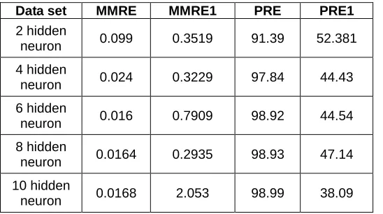
On comparing Multi Layer Preceptron, Radial Basis Function, Extreme Learning Machine, Support Vector Machine, and PSO in SVM, very good results are obtained at PSO in SVM

Data set MMRE MMRE1 PRE PRE1

2 hidden

neuron 0.099 0.3519 91.39 52.381 4 hidden

neuron 0.024 0.3229 97.84 44.43 6 hidden

neuron 0.016 0.7909 98.92 44.54 8 hidden

neuron 0.0164 0.2935 98.93 47.14 10 hidden

.PSO in svm has very low MMRE error value and is a very good optimization technique.

6

C

The results of this benchmarking study partially confirm the results of previous studies . Simple, understandable tech-niques like OLS with log transformation of attributes and target, perform as good as (or better than) non-linear tech-niques. Additionally, a formal model such as Cocomo per-formed at least equally good as OLS with log transformation on the Coc81 and Cocnasa data sets. These two data sets were collected with the Cocomo model in mind. However, this model requires a specific set of attributes and cannot be applied on data sets that do not comply with this re-quirement. Although the performance differences can be small in absolute terms, a minor difference in estimation performance can cause more frequent and larger project cost overruns during software development. Hence, even small differences can be important from a cost and opera-tional perspective .Another conclusion is that the selection of a proper estimation technique can have a significant im-pact on the performance. A simple technique like regression is found to be well suited for software effort estimation which is particularly interesting as it is a well documented technique with a number of interesting qualities like statis-tical significance testing of parameters and stepwise analy-sis. This conclusion is valid with respect to the different me-trics that are used to evaluate the techniques. Furthermore, it is shown that typically a significant performance increase can be expected by constructing software effort estimation models with a limited set of highly predictive attributes. Hence, it is advised to focus on data quality rather than col-lecting as much predictive attributes as possible. Attributes related to the size of a software project, to the development, and environment characteristics, are considered to be the most important types of attributes.

7

F

R

This study indicates that different data preprocessing steps, addressing possible data quality issues such as discretiza-tion algorithms, missing value handling schemas, and scal-ing of attributes, can play an important role in software effort estimation. While the same data preprocessing steps were applied on all data sets, the results of the input selection indicate that preprocessing steps such as attribute selection can be important. A thorough assessment of all possible data preprocessing steps seems however computationally infeasible when considering a large number of techniques and data sets. The impact of various preprocessing tech-niques has already been investigated to a limited extent, but further research into this aspect could provide important insights. This work can be extended using Genetic Algo-rithm, optimization can be applied to get the result for all methods. Also, considering the typical limited number of observations and the importance of expert knowledge (i.e. contextual information) for software effort estimation, we believe the inclusion of such expert knowledge to be a promising topic for future research. Now, this topic has been investigated only to a limited extent in software effort esti-mation. Future research could be done into these aspects by especially considering the impact such estimations can have on the budgeting and remuneration of staff.

R

[1] Jones, T.C. Estimating Software Costs, McGraw-Hill, 1998.

[2] Thayer, H.R., Software Engineering Project Management, Second Edition IEEE CS Press, 2001.

[3] C. Symons, “Come Back Function Point Analysis (Modernized) – All is Forgiven!”, Proc. of the 4th European Conference on Software Measurement and ICT Control, FESMA-DASMA 2001, pp. 413-426, 2001.

[4] C. M. Bishop, Neural networks for pattern recognition. Oxford J. M. Zurada, Introduction to artificial neural systems. Boston: PWS Publishing Company, 1995.

[5] B. D. Ripley, Pattern Recognition and Neural Networks. Cam-bridge University Press, 1996.

[6] G. Finnie, G. Wittig, and J.-M. Desharnais, “A comparison of soft- ware effort estimation techniques: Using function points with neural networks, case-based reasoning and regression models,” Journal of Systems and Software, vol. 39, pp. 281–289, 1997.

[7] C. Burgess and M. Lefley, “Can genetic programming improve software effort estimation? a comparative evaluation,” Informa-tion and Software Technology, vol. 43, pp. 863–873, 2001.

[8] M. Lefley and M. Shepperd, “Using genetic programming to improve software effort estimation based on general data sets,” in Lecture Notes in Computer Science, vol. 2724, 2003, pp. 2477–2487.

[9] K. Hornik, M. Stinchcombe, and H. White, “Multilayer feedfor-ward networks are universal approximators,” Neural Networks, vol. 2, no. 5, pp. 359–366, 1989.

[10]M. T. Hagan and M. B. Menhaj, “Training feedforward networks with the Marquardt algorithm,” IEEE Transactions on Neural Networks, vol. 5, no. 6, pp. 989–993, 1994.

[11]J. Moody and C. Darken, “Fast learning in networks of locally-tuned processing units,” Neural Computing, vol. 1, pp. 281–294, 1989.

[12]D. Specht, “A general regression neural network,” IEEE Trans-actions on Neural Networks, vol. 2, no. 6, pp. 568–576, 1991.

[13]A. Idri, A. Zahi, E. Mendes, and A. Zakrani, “Software Cost Esti-mation Models Using Radial Basis Function Neural Networks,” in Lecture Notes in Computer Science, vol. 4895, 2008, pp. 21–31.

[14]A. Heiat, “Comparison of artificial neural networks and regres-sion models for estimating software development effort,” Infor-mation and Software Technology, vol. 44, no. 15, pp. 911– 922, 2002.

[15]V. N. Vapnik, Statistical Learning Theory. New York, USA: John Wiley, 1998.

[17]V. Kumar, V. Ravi, M. Carr, and R. Kiran, “Software development cost estimation using wavelet neural networks,” The Journal of Systems and Software, vol. 81, pp. 1853–1867, 2008.

[18]G.-B. Huang, Q.-Y. Zhu, C.-K. Siew, “Extreme learning machine: a new learning scheme of feedforward neural networks”, in: Proceedings of International Joint Conference on Neural Net-works (IJCNN2004), 25–29 July, 2004, Budapest, Hungary.

[19]G.-B. Huang, Q.-Y. Zhu, K.Z. Mao, C.-K. Siew, P. Saratchandran, N.

[20]Sundararajan, “Can threshold networks be trained directly?”, IEEE Trans. Circuits Syst. II 53 (3) (2006) 187–191.

[21]I. Myrtveit and E. Stensrud, “A controlled experiment to assess the benefits of estimation with analogy and regression models,” IEEE Transactions on Software Engineering, vol. 25, no. 4, pp. 510–525,

[22]B. Littlewood, P. Popov, and L. Strigini, “Modeling software de-sign diversity a review,” ACM Computing Surveys, vol. 33, no. 2, pp. 177–208, 2001.

[23]R. M. Dawes, D. Faust, and P. E. Meehl, “Clinical versus actuar-ial judgement,” Science, vol. 243, no. 4899, pp. 1668–1674, 1989.

[24]M. Jørgensen, “Forecasting of software development work ef-fort: Evi- dence on expert judgement and formal models,” Inter-national Journal of Forecasting, vol. 23, pp. 449–462, 2007.