http://www.sciencepublishinggroup.com/j/sjams doi: 10.11648/j.sjams.20180603.13
ISSN: 2376-9491 (Print); ISSN: 2376-9513 (Online)
The Mutual Nearest Neighbor Method in Functional
Nonparametric Regression
Xingyu Chen
1, *, Dirong Chen
21
School of Mathematics and System Science, Beihang University, Beijing, P. R. China
2School of Mathematics and Computer Sciences, Wuhan Textile University, Wuhan, P. R. China
Email address:
*
Corresponding author
To cite this article:
Xingyu Chen, Dirong Chen. The Mutual Nearest Neighbor Method in Functional Nonparametric Regression. Science Journal of Applied Mathematics and Statistics. Vol. 6, No. 3, 2018, pp. 81-89. doi: 10.11648/j.sjams.20180603.13
Received: June 5, 2018; Accepted: July 12, 2018; Published: July 19, 2018
Abstract:
In recent decades, functional data have become a commonly encountered type of data. Its ideal units of observation are functions defined on some continuous domain and the observed data are sampled on a discrete grid. An important problem in functional data analysis is how to fit regression models with scalar responses and functional predictors (scalar-on-function regression). This paper focuses on the nonparametric approaches to this problem. First there is a review of the classical k-nearest neighbors (kNN) method for functional regression. Then the mutual nearest neighbors (MNN) method, which is a variant of kNN method, is applied to functional regression. Compared with the classical kNN approach, the MNN method takes use of the concept of mutual nearest neighbors to construct regression model and the pseudo nearest neighbors will not be taken into account during the prediction process. In addition, any nonparametric method in the functional data cases is affected by the curse of infinite dimensionality. To prevent this curse, it is legitimate to measure the proximity between two curves via a semi-metric. The effectiveness of MNN method is illustrated by comparing the predictive power of MNN method with kNN method first on the simulated datasets and then on a real chemometrical example. The comparative experimental analyses show that MNN method preserves the main merits inherent in kNN method and achieves better performances with proper proximity measures.Keywords:
Functional Data, Nonparametric Estimation, Mutual Nearest Neighbors Estimator, Semi-Metric1. Introduction
Regression is a well-known statistical problem, which consists in studying the link between the explanatory variable and the response variable. The regression function, which is most commonly the conditional expectation of the explanatory variable, is to be estimated in order to predict the response variable given a new value for the explanatory variable.
In the classical statistical setting, each observation is supposed to be a collection of numerical measurements represented by a p-dimensional vector. In practice, observations are observed at discrete sampling points. Thanks to technological progress, instants of measure come closer so grids are more and more fine. These practical improvements have naturally cast the regression problem into the general class of functional data analysis, where the
observation contains at least a functional object rather than standard vectors.
Functional data are intrinsically infinite dimensional. On the one hand, the infinite dimensional structure of the functional data is a rich source of information. On the other hand, the high intrinsic dimensionality of these data poses challenges both for theory and computation. The book of Ramsay and Silverman [1] provides a comprehensive introduction to the functional data analysis. Nonparametric ideas have been popularized by the book of Ferraty and Vieu [2]. A brief discussion of functional data analysis is presented by Wang et al. [3] and an introduction to recent advances in infinite dimensional statistics is presented by Goia and Vieu [4].
regression (scalar responses and functional predictors), function-on-scalar regression (functional responses and scalar predictors) and function-on-function regression (functional responses and functional predictors). The scalar-on-function regression has been applied in many domains and Reiss et al. [6] reviews some approaches to this regression problem. This article focuses on the nonparametric approaches to scalar-on-function regression.
The k-nearest neighbor (kNN) is one of the most famous nonparametric method. The first works were presented by Royall [7] and Stone [8], and the monograph by Györfi et al. [9] proposes a wide presentation on kNN ideas in nonparametric finite dimensional statistics. Starting with Laloë [10] and Burba et al. [11], there are some advances in kNN nonparametric functional data analysis, including the construction of the kNN kernel estimator of regression operator and some asymptotic results with convergence rates. The mutual nearest neighbors (MNN) method is a variant of kNN method. It takes use of the concept of mutual nearest neighbors rather than k-nearest neighbors to construct regression model. The term of mutual nearest neighbors seems to date back to Chidanand Gowda and Krihna [12] in the context of clustering. Liu et al. [13] apply mutual nearest neighbors to classification purposes and the experimental results show that the classification performance achieved by MNN method is better than the classical kNN method. Guyader et al. [14] investigates the theoretical properties of MNN method for the finite dimensional regression case.
This paper proposes the mutual nearest neighbors method in nonparametric functional regression setting. The organization of the paper is as follows. Section 2 presents MNN estimators based on a functional regression problem and some proximity measures. Section 3 shows the experimental results on the simulated datasets and then Section 4 shows that MNN method achieves a better performance on a real chemometrical example.
2. MNN Method and Proximity Measures
2.1. Models and Estimators
A random element is said to be functional if it takes its values in an infinite dimensional space. Many random elements, such as vectors of random curves, random surfaces and random fields of any dimension, enter this general definition. In this paper, functional data typically consist of a random sample of independent real-valued functions,
, … , , on a compact interval T on a real line. Such data have also been termed curve data.
The regression problem now is about linking the response to a whole curve observed on a domain T
X ≜ : ∈ T .
The random curve X is assumed to belong to a functional space ℱ. Therefore, the functional regression model we consider is
= r X + ε,
with ∈ ℝ and ε a scalar random disturbance such that
E ε|X = 0 almost surely. And now r ⋅ is an operator from
ℱ to ℝ satisfying some necessary regularity conditions. Let = X , , … , X , be a sample of the functional random variable X and response variable valued in ℱ × ℝ. Given a new observation curve x, our goal is to estimate the regression function r x = E[ |X = x] using the data ".
For a fixed x, reorder the data " according to the increasing values of d X , x , where d ⋅,⋅ is a function that defines the proximity between each pair of elements of a set. The reordered data sequence is denoted by
$X , x , , x % , … , $X , x , , x %.
If no confusion is possible, it can also be denoted by
$X x , x % , … , $X x , x %.
X& x is called the k-th nearest neighbor of x. If
d X , x = d X', x , then we have a tie. The tie breaking is done by indices, i.e., X might be declared "closer" if ( < *.
Let us denote +& x the set of the , nearest neighbors of x in ",
+& x = -X x , … , X. x /
For a fixed x ∈ ℱ, the kNN estimator can be written as
r0& x = 1 :23∈+45
.
From an optimal perspective, it is not a good idea to fix a globally optimal value of , for kNN in some real applications. For example, although an outlier is far from other curves, it may still treat some other curves as its nearest neighbors. Such pseudo neighbors are often found in the classical k-nearest neighbors. If they are used to predict the responses of new curves, the final results are doubtable in some way. Therefore, it would be better to exclude the pseudo neighbors from constructing regression models.
Given two parameters , and 6, let us denote +& x the set of the , nearest neighbors of x in , +7 x the set of the 6 nearest neighbors of X in \ X ∪ x . The set of the mutual nearest neighbors of x is
ℳ&,7 x = X : X ∈ +& x , x ∈ +7 X .
Denoting ;&,7 x = |ℳ&,7 x | the number of mutual nearest neighbors of x. For the sake of simplicity, , and 6 are usually assigned to the same value ,. Thus, ℳ&,7 x and
;&,7 x can be denoted as ℳ& x and ;& x respectively.
And then ;& x is a random variable taking values in
0,1, … , , .
An observation curve X is a mutual nearest neighbor of
of X= and X= appears in the k-nearest neighbors list of X at the same time. Obviously, X= is also a mutual nearest neighbor of X . It means that mutual nearest neighbors have symmetric property contrarily to the k-nearest neighbors.
If only the mutual nearest neighbors are used to construct the regression model, MNN regression estimate is defined as follows
r0> x =;1
& x :21 3∈ℳ45
with the convention that 0/0 = 0. It is an extension of kNN functional regression with mutual nearest neighbors. Because the pseudo neighbors of x have been eliminated and the rest are closer to itself, the MNN regression method is more reasonable than kNN regression method.
2.2. Proximity Measures
Generally, the performance of both nearest neighbors method heavily relies on the following three factors: the sample size ", the selection of proximity measure d ⋅,⋅ and the number of neighbors ,.
In the classical multivariate regression model, X is a p- dimensional vector of continuous covariates and r ⋅ is a smooth function from ℝ@ to ℝ. In this case, the proximity measure d ⋅,⋅ which is used to measure the distance between observations is the standard Euclidean metric of ℝ@. Thus, the distance between X and X' is
dAX , X'B = C D − D' =+ ⋯ + D@− D'@ =
where X = D , … , D@ G and X'= D' , … , D'@ G.
In the functional cases, the natural distance between elements are computed by means of the classical H=-metric, a generalization of the Euclidean metric, which is defined for all observed curves X and X' by
dAX , X'B = CI[ − ' ]=J . (1)
But sometimes, H=-metric may lead to terrible results in nonparametric functional cases.
The curse of dimensionality is strongly linked with the sparseness of data in a high-dimensional space. The concentration function L ℎ measures how densely packed are the considered elements of ℱ in an infinite dimensional ball of radius ℎ. For a fixed x ∈ ℱ, the value of the concentration function is estimated by
L05 ℎ = ∑ 1Q O 5,P X , (2)
where ℎ is a fixed bandwidth, the symbol 1 is an indicator function and R x, ℎ = xS: d x, xS < ℎ . Geenens [15] conjectures that the concentration function L ℎ typically decreases to 0 exponentially quickly as ℎ → 0 and the convergence of r0 toward r has unacceptable logarithmic rate in the functional space of interest, which is called as the curse
of infinite dimensionality. Concretely, for a fixed x, there are too few X close enough to x in the sense of H=-metric even when the sample size grows to infinity. And hence it is not reliable to make the estimation of r x using nearest neighbors.
On the other hand, the H=-metric just considers functions as infinite-dimensional vectors for it is the strict generalization of the Euclidean metric to functions. If the actual values taken by the functions are important for the problem, the H=-metric may be a good choice. But if only the shape of the functions is related to the response , the H=-metric may lead to bad conclusions. It can be explained that the H=-metric is probably too exacting to capture some of the features proper to functions, such as their general appearance, the way they vary over short or long range, etc.
Results of Ferraty and Vieu [2] show that it is wise to choose other looser proximity measures in place of H=-metric. The new proximity measures are expected to have the following two characteristics. First, it results in a new concentration function that decreases less rapidly as ℎ → 0. Therefore, more curves are close to each other so that more observations can contribute to the computation of r x . Second, it leaves out the irrelevant characteristics of the curves and highlights the particular characteristics of the curves that we know to be directly related to the response in the analysis.
It is a good idea to measure the proximity between two elements of the infinite dimensional functional space via a semi-metric, which is a metric except that d x, y = 0 ⇏ x =
y.
For instance, consider the following family of semi-metrics:
dWAX , X'B = CI[ W − 'W ]=J , (3)
where X takes values in 0,1,2, … . For any q-times differentiable real function x, x W denotes the q-th derivative of x . The main effect produced by the differentiating operator is to highlight some ranges of observed curves with large variations. The following example illustrated this effect.
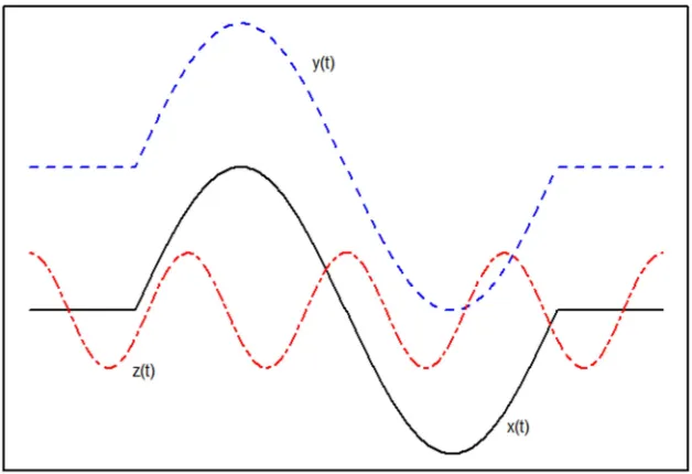
Consider the three functions D (black line), Z (blue dashed) and [ (red twodash) presented in Figure 1. Intuitively, the general appearance of D and Z is almost identical while D and [ are different. Based on the H=-metric, the distance between D and [ is smaller so that [ becomes the nearest neighbor of D . This may lead to a bad conclusion if the response is mainly related to the trend of curves, as Z is more helpful to the prediction procedure of D . In this case, the problem can be solved by the semi-metric based on the first derivatives:
d x, y = \][DS − ZS ]=J .
This looser proximity measure cancels out the vertical shift and care more about the shape of the curves. With this semi-metric d ⋅,⋅ , Z becomes the nearest neighbor of
Figure 1. Three curves: D (black line), Z (blue dashed) and [ (red two dash).
3. Simulation Experiments
In order to demonstrate the effectiveness of the MNN method, this section shows that how the MNN procedures work in a simple simulated finite sample situation. As mentioned in the previous section, the MNN method is an extension of kNN by using mutual nearest neighbors. Thus a comparison between the classical kNN method and MNN method is designed in this section.
We simulate " =300 pairs X , Q . The sampled functional explanatory variables are generated as follows, for each ( 1,2, … ,300 :
X _ cos 2 , 0, c!
where
_ ~e 0,1 for ( 1,2, … ,150,
_ ~e 3, h= for ( 151, … ,300.
Different values for h= will create two groups of curves inside the dataset with concentration being different from one group to the other one. In this simulation study, two extreme cases are considered, the most homogeneous one when
h= 1 and the most heterogeneous one when h= 0.1. The
curves X , … , X are observed on the same grid generated from 100 equispaced measurements in 0, π! and displayed in Figure 2. (Note that these cases are the same as the cases in Burba et al. [7].)
Figure 2. The simulated curves with h= 1 (left panel) and the simulated curves with h= 0.1 (right panel).
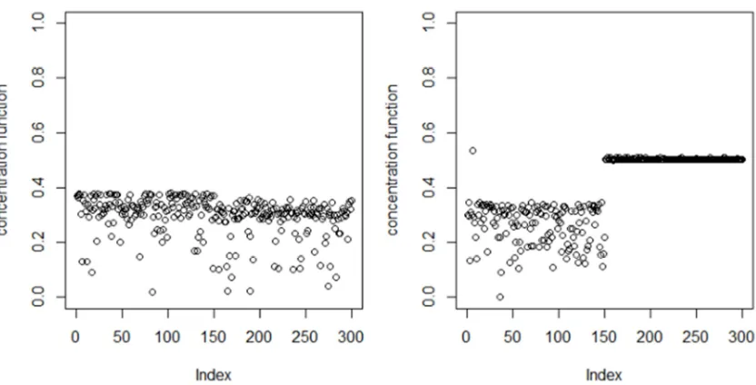
Here the notions of homogeneity and heterogeneity will refer to the concentration of the data. The concentration function L M , which can be estimated the values by (2), illustrates the difference between the two datasets. Usually, the bandwidth M is obtained by a cross-validation procedure but other values of M have similar results in fact. Here 0.7 is
Figure 3. Values of concentration function with ℎ =0.7 (left: h= 1; right: h= 0.1).
The aim is to study the following functional nonparametric regression model:
r X k ,
where the k’s are generated independently according to a
e 0,0.05 distribution and are assumed to be independent of
X for all ( 1,2, … , " . We will observe the behavior of the two methods (MNN method and kNN method) in these two extreme cases. The nonparametric regression operator r x is
r X _=, ( 1, … , ".
In both cases 150 curves will be randomly taken to construct the training sample lmno and the other 150 will constitute the testing sample lmpqm . Both kNN-based estimators and MNN-based estimators depend on the quantity of neighbors , which must be selected from the training sample. And the testing sample is used to measure the accuracy of the predictions. The proximity is measured by the classical H=-metric.
The optimal number of neighbors ,r@m is obtained by minimizing a global cross-validation criterion on the training sample, that is:
,r@m arg min& xy ,
where
xy , 1z E r0{ X |=
Q
with
r0{ x 1
,':' +1 '
45 ,'}
for kNN-based estimator and
r0{ x 1
;& x ':' :1 '
45
for MNN-based estimator. Noting that the optimal number of neighbors ,r@m or these two methods are different in most times.
Some results of predictions are presented here. Note that MSEP is the mean square error of prediction, that is
MSEP # l1
mpqm 1 E ‚
=
ƒ„…†„
,
where # lmpqm denotes the quantity of the testing sample and
‚ denotes a prediction of . Here # lmpqm is 150.
Figure 4. Knn method vs. mnn method in the most homogeneous case.
Figure 5. Knn method vs. mnn method in the most heterogeneous case.
It is obvious that for the kNN method, there is a deviation between ‚ and when the true value locates at the boundary of the range. This is due to the fact that the , nearest training samples are used to predict the response of the curve we concern in kNN method. When the curve, represented by x‡, locates at the boundary, the majority of the training samples are on the same side of x‡. If the k-th nearest training sample is far away from x‡, the deviation could not be avoided.
But for the MNN method, the deviation is not obvious. The MNN method takes use of the concept of mutual nearest neighbors rather than , nearest neighbors of x‡ to predict its values. The sample curves which are far away from x‡ may be excluded so that they will not be taken as determinant conditions. Thus, the final prediction results for MNN method
don’t have obvious deviation.
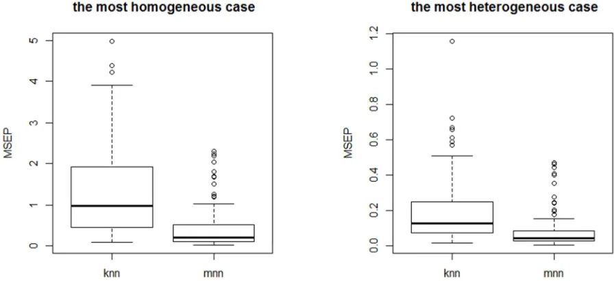
Replicate the experiment M 100 times and then M samples X , Q are drawn. Each of the M simulated datasets are randomly split into two sample: a training sample
lmno contained 150 curves and a test sample lmpqm contained other 150 curves. From each training sample and or both kNN and MNN methods, the tuning parameter , is selected by means of the global cross-validation procedure and (
Figure 6. Mean square errors of prediction from the M = 100 replicates of the experiment. Left panel: h==1 (the most homogeneous case). Right panel: h= 0.1 (the most heterogeneous case).
4. A Real Dataset Application
The aim of this section is to compare the predictive power of the MNN method and kNN method on a real dataset. We focus here on a quality control problem in the food industry. The dataset concerns a sample of finely chopped meat and is a part of Tecator dataset, which can be found at http://lib.stat. cmu.edu/datasets/tecator.
The dataset consists in N 215 observations. For each meat sample i, the data consists of a 100 channel spectrum of absorbance X and the contents of fat . The absorbance is -ln10 of the transmittance measured by the spectrometer and the data were recorded on a Tecator Infractec Food and Feed Analyzer working in the wavelength range 850 − 1050 nm by the near-infrared (NIR) transmission principle. Because of the fineness of the grid, each sample can be considered as a
continuous curve although it appears clearly as a discretized curve. The spectrometric curves are presented in the left panel of Figure 7. The content of fat, measured in percent, is determined by analytic chemistry. The task is to predict the fat content of a meat sample on the basis of its near infrared absorbance spectrum.
To compare the predictive power of each functional regression method (kNN and MNN), this sample of size 215 was splitted into a learning sample of size 120 and a testing sample of size 95. First, consider the partition given by
lmno 1,2, … ,120 and lmpqm 121, … ,215 to obtain a
proper proximity measure. The H=-metric, quantifying in a sense the area between the curves, focuses on the vertical shifts among curves and thus lead to poor predictions. The MSEP with the H=-metric for MNN method is 138.57.
Figure 7. Absorbance curves (left panel) and their second derivatives (right panel).
Since the smoothness of the curves, we consider the family
of semi-metrics based on the derivatives, dW , , X 1,2,3,4
when estimating from kNN and MNN-based estimators. The corresponding optimal number of neighbors ,r@m is obtained by minimizing a global cross-validation criterion as in the simulated example before. Keep in mind that with a functional linear model, i.e., a model which does not involve any nonparametric component, the MSEP is 7.17. This value can serve as a benchmark for analyzing the results in Table 1. Table 1 indicates that the most suitable proximity measure is the semi-metric based on the second order derivatives:
d=AX , X'B \] = E '= !=J .
The second derivatives of the absorbance curves are
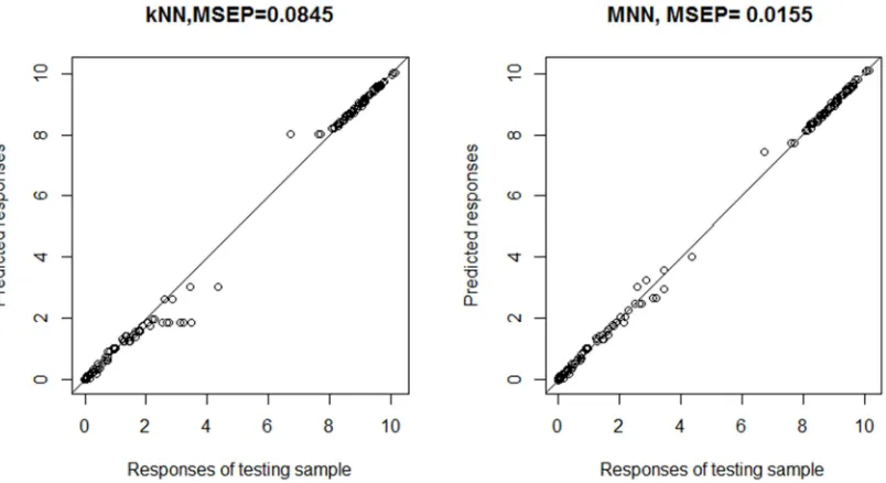
displayed in the right panel of Figure 7. Figure 8 displays the predicted values obtained by the two methods (kNN and MNN) on the testing sample with the semi-metric d= , The MNN method shows the better predictive power with a MSEP of 3.4294 (against 6.7480 for the kNN method).
Table 1. The selected semi-metric (X0) and the values of MSEP for kNN and MNN method.
Š‹ kNN MNN
1 16.3255 11.4630
2 6.7480 3.4294
3 14.3117 14.4158
4 11.2274 7.3261
Figure 8. Knn method vs. mnn method for predicting fat content from spectrometric curves using the semi-metric based on the second derivatives.
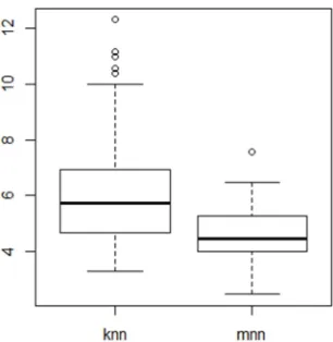
Figure 9. Boxplot of 100 values for the MSEP.
We only use a particular partition in the first attempt. To attenuate the effect of the considered partition, 100 partitions are generated at random. The semi-metric based on the second order derivatives has the best results and thus we use it as the proximity measure here. From each training sample and for both kNN and MNN methods, the tuning parameter , is
chosen as before and then ( lmpqm is predicted. 100 values for the MSEP are obtained for each method and displayed as the boxplots in Figure 9. It clearly shows a better predictive power for the MNN method.
5. Conclusion
References
[1] Ramsay J O, Silverman B W. Functional Data Analysis [M]. Springer New York, 1997.
[2] Ferraty F, Vieu P. Nonparametric functional data analysis: theory and practice [M]. Springer New York, 2006.
[3] Goia A, Vieu P. An introduction to recent advances in high/infinite dimensional statistics [J]. Journal of Multivariate Analysis, 2016, 146 (2):1-6.
[4] Wang J L, Chiou J M, Mueller H G. Review of Functional Data Analysis [J]. Statistics, 2015.
[5] Morris J S. Functional regression [J]. Annual Review of Statistics and Its Application, 2015, 2: 321-359.
[6] Reiss P T, Goldsmith J, Shang H L, et al. Methods for Scalar‐ on-Function Regression [J]. International Statistical Review, 2017, 85 (2): 228-249.
[7] Royall R M. A class of non-parametric estimates of a smooth regression function [D]. Department of Statistics, Stanford University, 1966.
[8] Stone C J. Consistent nonparametric regression [J]. The annals of statistics, 1977: 595-620.
[9] Györfi L, Kohler M, Krzyzak A, et al. A distribution-free theory of nonparametric regression [M]. Springer Science & Business Media, 2006.
[10] Laloë T. A k-nearest neighbor approach for functional regression [J]. Statistics & probability letters, 2008, 78 (10): 1189-1193.
[11] Burba F, Ferraty F, Vieu P. k-Nearest Neighbour method in functional nonparametric regression [J]. Journal of Nonparametric Statistics, 2009, 21 (4): 453-469.
[12] Gowda K C, Krishna G. Agglomerative clustering using the concept of mutual nearest neighbourhood [J]. Pattern recognition, 1978, 10 (2): 105-112.
[13] Liu H, Zhang S, Zhao J, et al. A new classification algorithm using mutual nearest neighbors [C]. Grid and Cooperative Computing (GCC), 2010 9th International Conference on. IEEE, 2010: 52-57.
[14] Guyader A, Hengartner N. On the mutual nearest neighbors estimate in regression [J]. The Journal of Machine Learning Research, 2013, 14 (1): 2361-2376.