NUMERICAL SIMULATION OF THE METHANE INJECTION PROCESS IN THE INLET MANIFOLD OF A DIESEL ENGINE

(1)

NUMERICAL SIMULATION OF THE METHANE INJECTION PROCESS IN THE

INLET MANIFOLD OF A DIESEL ENGINE

Ass.Prof. PhD Evtimov T.,

Faculty of Transport – Technical University of Sofia, Bulgaria E-mail: [email protected]

Abstract: The main purpose of this paper is a numerical simulation of methane injection process in the inlet manifold of a compression ignition engine. The paper gives an overview of issues related to the turbulence modeling. Computational resources such as the amount of time for the simulation and the memory of the individual models were discussed. While it is impossible to state categorically which model is the most appropriate for a specific application, general guidelines are presented in order to help you choose the turbulence model for the flow you want to model.

KEYWORDS: TURBULENCE MODELING, GOVERNING EQUATIONS, NUMERICAL SIMULATION, DIESEL ENGINE

1. Introduction

Turbulent flow is characterized by a variable-speed field. The flows carry quantities of pulse, energy and mass and simultaneously are the cause of their change.

It is a fact that there is no single universal turbulent model applicable to all types of tasks. The choice of turbulent model will depend on the physical processes occurring in the flow, of the method used, the degree of accuracy, of the computational resources and the time for the simulation. [1]

The system of equations of Navier-Stokes describe the flow fully [2] . The numerical methods which are used for direct solving of these equations are called direct numerical simulations (DNS). Turbulent flows, however, are usually characterized by eddies of various duration in time and with different linear dimensions determined by the acting forces. The results from DNS can be used for verification of the various models of the turbulence. The solving of the averaged equations of Navier-Stokes, instead of momentary, reduces the computational effort to acceptable levels. In the averaged equations unspecified members are appearing. The different models of the turbulence that solve this task can be classified according to the limit linear dimensions

∆

f

, at which the averaging is introduced. All physical processes that take place in linear dimensions greater than

∆

f

are covered by the averaged equations of Navier-Stokes. In this way can be resolved also those with linear dimensions smaller than

∆

f

, as the undetermined members of the averaged equations are described by modeling.

For calculations in direct numerical simulations (DNS), the limit linear dimensions are smaller than those of the Kolmogorov,

η

<

∆

f

it is therefore not necessary to introduce modeling. If the limit value is equal to the integral linear dimension,

∆

f

=



, the turbulence model is called a model of Navier-Stokes averaged by the method of Reynolds (RANS).

Widespread and used is the model

k

−

ε

, which belongs to this category. If the limit linear size is between

η

and



,



<

∆

<

f

η

model is called model for large eddy simulation (LES). Williams [4] proposed an extension of the

k

−

ε

model by reducing its limit linear size below



[2]. This model of the type of very large eddy simulation (VLES), includes the properties of LES

models in

k

−

ε

model and thereby is covering a wider range of the dynamics of the turbulence and at the same time is maintaining the computing efforts at an acceptable level.

2. Physical models

The considered several models can be used to describe the different physical processes in simulations of diesel engine with

internal combustion (DEIC). These models are associated with the equations describing the processes meet the required mathematical requirements for simulating processes DEIC [3].

For the most common statistical 3-D flow there are four independent equations describing the main velocity field, namely the three components of the averaged equations for the velocity together with the basic equation of the continuity (or Poisson equation for pressure). There are also more than four unknowns, i.e. the three components of the velocity, pressure and the components

in the member

ρ

u

~



u

~



. These components are related to the stress of Reynolds, resulting from the transmission of the impulse from the changing velocity field. Since the number of unknowns is greater than the number of equations, a problem occurs at the completion of the system of equations. To complete the system is used the hypothesis for relatively distribution. This hypothesis is

applied to the members

ρ

u



"

E

"

and

ρ

u



"

Y

_i

"

in the equations of energy conservation and the equations for conservation of mass or for each one of the components

K

as:

K

Γ

u

"

φ

"

=

−

_K_,_T

∇

~

ρ



(1).

The effective diffusion coefficient

Γ

_K_,_eff is defined as the sum of the molecular

Γ

_K and turbulent

Γ

_K_,_T components. Diffusion coefficients corresponding to the transfer of mass, energy and momentum are shown in Table 1.

Table 1: Coefficients of turbulent exchange

Transferred amount

Mass Energy Impulse

Coefficient of

transfer

Γ

Yi,T

Γ

E,T

Γ

T

Symbol

T

D

K

_T

/

c

_P

ν

_T

Formula

(

)

T T

/

ρ

Sc

µ

_T

/

Pr

_T

µ

_T

/

ρ

In the above diffusion coefficients, the values of the turbulent

numbers of Prandtl

Pr

_T

=

0 ,

56

and Schmidt

Sc

_T

=

0 ,

9

. Similarly to the equations for the mass and energy, the hypothesis of the turbulent viscosity introduced by Boussinesq is mathematically analogous to the relationship between the pressure and the rate of deformation for a Newtonian fluid. In conclusion, the stresses of Reynolds can be written as:

u



"



"

=

−

ρ

ν

_T

∇

~



ρ

(2)

• algebraic models (universal model of turbulent viscosity, model for mixed lengths);

• models with one equation;

• models with two equations (standard

k

−

ε

model and RNG

k

−

ε

model)

• Reynolds Stress Model (RSM).

2.1.

k

−

ε

model of the turbulence

In this model are solved two additional equations for the transfer of both turbulent components - the turbulent kinetic energy

k

~

and the rate of energy diffusion

ε

~

. These two components refer to the original variables and they can determine

k

−

ε

linear size and length of time for the formation of quantity with dimension of

T

ν

, and in this way they turn the model into a complete one. This is widely used model for calculation of fluid dynamics (CFD).

2

1 "

u

~

k

~

=

(3)

"

u

:

"

u

~

=

ν

∇



T

∇



ε

(4)

ε

ν

T

C

_µ

k

~

_~

2

=

(5)

The equation for the balance of

k

~

can be obtained from equations (3), (4), (5) and the equation for conservation of the momentum:

( )

₍

₎

0 .

.

⊗

−

∇

=

∇

+

=

∇

+

∂

S

F

g

p

u

t

u



_ρ



_σ

_ρ



_

ρ

The result is:

( )

S k eff

W

k

u

k

u

t

k





+

−













∇













∇

+

∇

+

∇

−

=

∇

+

∂

ε

ρ

µ

σ

ρ

~

Pr

.

~

:

~

.

~

3

2 ~

~

.

~

(6)

( )

[

S

]

S eff

W

c

u

c

k

u

c

u

t





+

−

∇

+













∇













∇

+

∇













₋

−

=

∇

+

∂

ε

ρ

σ

ε

µ

ε

ρ

ε

ρ

ε

ρ

ε ε ε ε ε

~

:

~

Pr

.

~

.

~

3

2 ~

~

.

~

2 1 3 1 (7)

The flow in the internal combustion engine (ICE) has a variable density, which leads to a change in the volume of the infinitesimal element. This process is called velocity expansion. The

member













₋

3 1

3

2

ε ε

c

in

ε

the equation is for tacking into

account the change in the linear dimensions due to the velocity

expansion. The member

W



Sis due to the interruption of the flow. The new quantities introduced by these equations are constants whose values are determined by some experimental and theoretical considerations. The standard values which are used for calculation of the internal combustion engine are shown in Table 2.

Table 2: Values of the constants in the models of the turbulence.

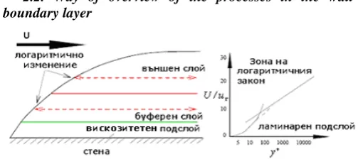
2.2. Way of overview of the processes in the wall boundary layer

Fig. 1 The area of logarithmic law and laminar sublayer of the wall

boundary layer are displayed.

The described in this way methods of examining of the turbulence in the wall boundary layer are valid mainly for homogeneous flow. The type of the flow near the wall requires more attention in the mathematical modeling due to the smaller line dimensions. Near the wall, the flow is divided into inner layer with prevailing viscosity phenomena and an outer layer, where these phenomena are not so significant (separated by the red line, see Figure 2). The layer very close to the wall in the inner layer (below the green line, see Figure 2) is called viscosity or laminar sublayer. The transition from one to the other layer is realized on logarithmic curve. While the change in the speed in the normal direction (perpendicular to the wall) vary linearly with a distance

y

from the wall in the laminar sublayer it is amended logarithmically. The numerical solution of the equations of the turbulence model in the wall boundary layer is not possible. It is needed more simple function that describes the flow between the last point of the network close to the wall and the wall. Such a function can be obtained through several simplifying assumptions for the flow in the wall boundary layer:

1. The flow is quasi-stationary.

2. The fluid velocity is parallel to the flat wals and vary only in the normal direction.

3. There is no change of the pressure in the flow.

4. In the area near to the wall no chemical reaction occurs and there is no source of injection.

5. The heat losses of the wall are smaller in comparison with the universal.

6. Reynolds numbers are higher (the dynamic viscosity is greater than the laminar viscosity) and the Mach numbers are smaller.

Thus,

k

−

ε

the equations can be written again in accordance with the already said assumptions and in non-dimensional form

using the friction velocity (velocity in the wall)

u

_W determined by

W W W

u

ρ

τ

=

(8), where

τ

_W is the tension in the wall boundary

layer and

ρ

_W is the density of the wall.

k

is non-dimensional due to the application of

u

_W2 , and

ε

due to the application of

y

/

u

_W3 , where

y

is the distance along the normal to the wall. Near the wall of the equations for maintaining the components in the other directions (

x

and

z

) disappear leaving only the equations for the direction

y

. These equations are:

Константа

1 ε

c

ε2

c

ε3

c

S

Pr

k

Pr

ε

η

0

β

c

µ

Стандартен

ε

−

k

1,44 1,92 -1,0 1,5 1,0 1,3 - - 0,09

(3)

1

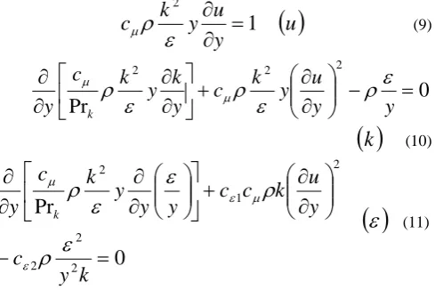
2

=

∂

y

u

y

k

c

ε

ρ

µ

( )

u

(9)

0 Pr

2 2

2

=

−













∂

+













∂

y

u

y

k

c

y

k

y

k

c

y

k

ε

ρ

ε

ρ

ε

ρ

µ

( )

k

(10)

0 Pr

2 2

2

1 2

=

−













∂

+

























∂

k

y

c

y

u

k

c

y

k

c

y

_k

ε

ρ

ε

ρ

ε

µ ε µ

( )

ε

(11)

The solution of these equations for

u

,

k

and

ε

is performed by using Taylor series and in the result is received the the speed of distribution in the wall boundary layer:

B

y

ln

u

=

+

κ

1

0 (12)

B

yu

c

ln

u

L W W

+

























=

8

7

1

1 ν

κ

(13)

Where

κ

is called von Karman constant and has a value of 0,4372 [3] for values of the constants of the model shown in Table 2,

B

=5,5 for smooth walls [3]. The above function is called the law of the wall and because of its logarithmic character, the border area is called the zone of the logarithmic law. In the laminar sublayer, the velocity is calculated by using

2 1













=

L W

yu

u

ν

(14)

A correction is made of the places where equation (13) and

equation (14) contain the same

u

_W. For the given constants

144 u

_W

=

. The calculated velocities for the point of the network closest to the wall is connected with the values calculated by using the functions of the wall. In the final numerical performance is calculated the tangential velocity in the last cell in

the vicinity of the wall. This is used to determine the value of

u

_W, by using the equations (8) и (13). The heat exchange in the zone adjacent to the wall is done in a similar manner.

Fig. 2 Turbulent flow in the filler collector of a diesel engine with

use of the model

k

−

ε

2.3.RNG

k

−

ε

model of the turbulence

The idea of the renormalization group theory (RNG) is using a random universal force that causes fluctuations of small dimensions. This force represents the impact of larger sizes (including internal and boundary conditions) on the eddies in the inertial range. It is selected in such a way that the global characteristics of the resultant field of the flow are the same as those in the flow driven by the main tension. The equations of the motion for fields with large dimensions are obtained by averaging the infinitely small areas (strips) of the small dimensions in order to be removed. The process of elimination is repeated until infinitely small corrections of the equations are accumulated. The influence of the small dimensions, which have been removed is taken into consideration by dynamic equations for large dimensions of the velocity field due to the presence of the eddies. At the border where successively are eliminated the larger dimensions is obtained

ε

−

k

model.

This procedure covers only the conversion of the viscosity. After complete the elimination of the small dimensions, the random force is excluded from the resulting equations and the internal and boundary conditions are resumed. RNG procedure increases the number of equations, which do not contain undefined constants and the presence of correction. These equations allow the use of the model for the two ranges of the flow - with large and small numbers of Reynolds. The turbulence in ICE is characterized by large changes in density, even at small Mach numbers. In order to adjust the equation for

ε

of the RNG model for the cases of compressible flow the Rapid Distortion Analysis is used. The final equation for

ε

contains additional member and extra constant [3]:

ε

−

k

model applies mainly to the significant values of the relation between the duration of action of the tension in turbulence and the main tension caused by the injection.

In the most general case,

k

−

ε

models contain constants that depend on the geometry and type of the flow, but may determine the main speeds with sufficiently good accuracy. It is however important to note that the hypotheses for the transmission of the components are not the same for all types of turbulent flows [3]. The alternative Reynolds stresses models (RSM) are more accurate in predicting the energy levels in anisotropic turbulent flows. RSM requires a solution of seven additional equations (six for shear stresses for each surface of the element and one member for the diffusion), characterized by a greater calculation intensity. RNG

ε

−

k

model is proved to be particularly suitable for ICE in which the fuel injections lead to high values of the stresses [3].

(4)

2.4. Real /actual/ (Realizable)

k

−

ε

model of the turbulence

The real

k

−

ε

model is a relatively new development and differs from the standard

k

−

ε

model by two main features:

• The real

k

−

ε

model contains a new formulation for the turbulent viscosity;

• A new equation for the diffusion level is derived

ε

. The term "real" means that the model satisfies the precise mathematical limitations on Reynolds stresses related to the phenomena of turbulent flows. Neither the standard

k

−

ε

, nor the RNG

k

−

ε

models are completely real.

The immediate benefits of the real

k

−

ε

model is that it more accurately predicts the extent of spreading of both - planar and cylindrical jets. It is also possible to provide the better quality of implementation for flows involving rotation, boundary layers under strong counter pressure gradients, separation and recirculation.

Both the real and RNG

k

−

ε

model show significant improvements over the standard

k

−

ε

model, where the flow properties include highly distorted currents, eddies and rotations. Because the model is relatively new it is not clear in which cases it outperforms the RNG

k

−

ε

model. Initial studies indicate that the real model provides the best performance of all

k

−

ε

versions for some individual flows and flows with complex secondary properties.

use of the model Realizable

k

−

ε

2.5. Reynolds stresses model (RSM)

Reynolds stresses model is the most detailed model of the turbulence. By excluding the hypothesis for the viscosity of the eddies, RSM provides a solution to the equations of Navier-Stokes, averaged by the method of Reynolds, by solving the equations for transferring of Reynolds stresses, together with one equation for the diffusion rate.

This means that we need 4 additional equations for 2-D flows and 7 additional equations for the transmission for 3-D flows.

Since RSM is taking into account the impact of the turbulent currents, eddies, rotations and rapid changes in the level of tension more accurately than the models with 1 and 2 equations, it has a greater potential to make more accurate predictions for complex flows. The accuracy of the predictions of RSM, however, is still

limited because of the assumptions made in the modeling for the convergence of various members in precisely defined equations for transfer of the Reynolds stresses. Modeling of stresses and the level of diffusion is particularly challenging and often requires achieving of compromise with the accuracy of the RSM prediction.

RSM can not always lead to results that are superior to the simpler models.

However, the use of RSM is mandatory when the flow properties are the result of anisotropy in the stresses of Reynolds. Such are hurricane flows, highly turbulent flows in the combustion chamber, rotating currents and streams causing tensions in the channels.

use of the Reynolds (RSM) model

2.6. Model of the type of very large eddies simulation (VLES)

The displayed model of the VLES type is developed by Williams [4]. It is based on two-dimensional assessment which combines the components in at integral size



with those at average filtrating size

∆

_f in the inertial sub-range. The model is based on

k

−

ε

model shown above, but in addition it directly solves the turbulent structures with dimensions smaller than



, but still larger than

∆

_f, which can not be solved numerically by

ε

−

k

model. In order to achieve this the numerical dimension of the net must be compared with the filter dimension

∆

_f. Only the resulting equations of the model are shown. Instead of solving the entire system of equations for transfer only for a one particular level of the linear dimensions, the second level of linear dimensions is

used. Yet

k

~

and

ε

~

equations are solved with the integral linear

dimension



, while all other differential equations are solved with the filter dimension

∆

_f,

η

<

∆

f

<



. In order to use these two levels of the network should be used procedures called scaling up,

for passage from

∆

_f to



, and scaling down for passage from



to

∆

_f respectively.

For the model of the type VLES the following important features can be noted:

(5)

certainly avoiding the effect of suppression of the important turbulent structures inherent to the standard

k

−

ε

model. Its major disadvantage, in comparison with the standard

k

−

ε

model is the fact that it in order to obtain the average components statistical analysis of the results should be carried out. By combining the characteristics of the standard

k

−

ε

model with those of the LES model, the calculation efforts are maintained at an acceptable level.

the use of VLES model

3. Results

For carrying out the Numerical analysis of the process of

methane injection

(

CH

₄

)

in the filler collector of a diesel engine the program FLUENT6.2.1 is used. Calculations are performed under the following boundary conditions:

;

/

,

250 ;

/

,

50 ;

,

300 ;

,

101325

;

,

300

4 , 0 0

s

m

s

m

K

T

Pa

p

K

T

CH inj air

wall

=

υ

The results of the study of the applied different mathematical models are shown in the corresponding Figures.

4. Conclusions

• For the study of the processes occurring in the filler collector of DEIC while injecting methane in it the most appropriate turbulent model is the LES - model which avoids the effect of suppression of the important turbulent structures inherent to the

standard

k

−

ε

model;

• To obtain a numerical solution of the equations of the model of the turbulence in the wall boundary layer it is necessary to apply simplifying assumptions for the flow in the wall boundary layer;

• 2–D (

k

−

ε

) models are preferred over 3-D (LES) models in case of insufficient resources of calculation time and in solving a certain type of tasks;

• in studying the influence of the angle of the methane injection in the filler collector of DEIC over the mixture preparation process, the best mixture formation is observed at an angle equal to 60 degrees;

• the optimal combustion process is expected at maximum intensity of the turbulent flow that occurs in the LES model.

Bibliography

[1] http://bubble.me.udel.edu/wang/teaching/MEx81/fluent-help/html/ug/main_pre.htm

[2] Marcus Guido Herrmann, “Numerical Simulation of Premixed Turbulent Combustion

Based on a Level Set Flamelet Model”, 2001.

[3] Aglave R., “CFD Simulation of Combustion Using Automatically Reduced Reaction Mechanisms: A Case for Diesel Engine”, 2007

[4] W. Willems. Numerische Simulation turbulenter ScherstrÄomungen mit einem Zwei-Skalen Turbulenzmodell. PhD thesis, RWTH Aachen, 1996.