RESEARCH
An average-case sublinear forward
algorithm for the haploid Li and Stephens
model
Yohei M. Rosen
1,2*and Benedict J. Paten
2Abstract
Background: Hidden Markov models of haplotype inheritance such as the Li and Stephens model allow for compu-tationally tractable probability calculations using the forward algorithm as long as the representative reference panel used in the model is sufficiently small. Specifically, the monoploid Li and Stephens model and its variants are linear in reference panel size unless heuristic approximations are used. However, sequencing projects numbering in the thou-sands to hundreds of thouthou-sands of individuals are underway, and others numbering in the millions are anticipated. Results: To make the forward algorithm for the haploid Li and Stephens model computationally tractable for these datasets, we have created a numerically exact version of the algorithm with observed average case sublinear runtime with respect to reference panel size k when tested against the 1000 Genomes dataset.
Conclusions: We show a forward algorithm which avoids any tradeoff between runtime and model complexity. Our algorithm makes use of two general strategies which might be applicable to improving the time complexity of other future sequence analysis algorithms: sparse dynamic programming matrices and lazy evaluation.
Keywords: Forward algorithm, Haplotype, Complexity, Sublinear algorithms
© The Author(s) 2019. This article is distributed under the terms of the Creative Commons Attribution 4.0 International License (http://creat iveco mmons .org/licen ses/by/4.0/), which permits unrestricted use, distribution, and reproduction in any medium, provided you give appropriate credit to the original author(s) and the source, provide a link to the Creative Commons license, and indicate if changes were made. The Creative Commons Public Domain Dedication waiver (http://creat iveco mmons .org/ publi cdoma in/zero/1.0/) applies to the data made available in this article, unless otherwise stated.
Background
Probabilistic models of haplotypes describe how varia-tion is shared in a populavaria-tion. One applicavaria-tion of these models is to calculate the probability P(o|H), defined as the probability of a haplotype o being observed, given the assumption that it is a member of a population rep-resented by a reference panel of haplotypes H. This com-putation has been used in estimating recombination rates [1], a problem of interest in genetics and in medicine. It may also be used to detect errors in genotype calls.
Early approaches to haplotype modeling used
coales-cent [2] models which were accurate but
computation-ally complex, especicomputation-ally when including recombination. Li and Stephens wrote the foundational computationally tractable haplotype model [1] with recombination. Under their model, the probability P(o|H) can be calculated
using the forward algorithm for hidden Markov models (HMMs) and posterior sampling of genotype probabili-ties can be achieved using the forward–backward algo-rithm. Generalizations of their model have been used for haplotype phasing and genotype imputation [3–7].
The Li and Stephens model
Consider a reference panel H of k haplotypes
sam-pled from some population. Each haplotype hj∈H is a sequence (hj,1,. . .,hj,n) of alleles at a contiguous sequence 1,. . .,n of genetic sites. Classically [1], the sites are bial-lelic, but the model extends to multiallelic sites [8].
Consider an observed sequence of alleles
o=(o1,. . .,on) representing another haplotype. The
monoploid Li and Stephens model (LS) [1] specifies a
probability that o is descended from the population
rep-resented by H. LS can be written as a hidden Markov
model wherein the haplotype o is assembled by
copy-ing (with possible error) consecutive contiguous subse-quences of haplotypes hj ∈H.
Open Access
*Correspondence: [email protected]
Definition 1 (Li and Stephens HMM) Define xj,i as
the event that the allele oi at site i of the haplotype o was copied from the allele hj,i of haplotype hj∈H . Take parameters
and from them define the transition and recombination probabilities
We will write µi(j) as shorthand for p(oi|xj,i) . We
will also define the values of the initial probabilities p(xj,1,o1|H)= µ1k(j) , which can be derived by noting that if all haplotypes have equal probabilities 1
k of randomly
being selected, and that this probability is then modified by the appropriate emission probability.
Let P(o|H) be the probability that haplotype o was pro-duced from population H. The forward algorithm for hid-den Markov models allows calculation of this probability in O(nk2) time using an n×k dynamic programming
matrix of forward states
The probability P(o|H) will be equal to the sum
jpn[j] of all entries in the final column of the dynamic program-ming matrix. In practice, the Li and Stephens forward algorithm is O(nk) (see "Efficient dynamic programming"
section).
Li and Stephens like algorithms for large populations
The O(nk) time complexity of the forward algorithm
is intractable for reference panels with large size k. The
UK Biobank has amassed k =500, 000 array samples.
Whole genome sequencing projects, with a denser dis-tribution of sites, are catching up. Major sequencing projects with k=100, 000 or more samples are nearing
completion. Others numbering k in the millions have
been announced. These large population datasets have significant potential benefits: They are statistically likely to more accurately represent population frequencies and
(1) ρi∗−1→i probability of any recombination
between sitesi−1 andi
(2)
µi probability of a mutation from
one allele to another at sitei
(3) p(xj,i|xj′,i−1)
=
1−(k−1)ρi ifj=j′
ρi ifj�=j′ whereρi=
ρ∗i−1→i
k−1
(4) p(oi|xj,i)
=
1−(A−1)µi ifoi=hj,i
µi ifoi�=hj,i
whereA=number of alleles
(5) pi[j] =P(xj,i,o1,. . .,oi|H)
those employing genome sequencing can provide phas-ing information for rare variants.
In order to handle datasets with size k even fractions of these sizes, modern haplotype inference algorithms depend on models which are simpler than the Li and Stephens model or which sample subsets of the data. For example, the common tools Eagle-2, Beagle, HAPI-UR and Shapeit-2 and -3 [3–7] either restrict where recom-bination can occur, fail to model mutation, model long-range phasing approximately or sample subsets of the reference panel.
Lunter’s “fastLS” algorithm [8] demonstrated that hap-lotypes models which include all k reference panel haplo-type could find the Viterbi maximum likelihood path in time sublinear in k, using preprocessing to reduce redun-dant information in the algorithm’s input. However, his techniques do not extend to the forward and forward– backward algorithms.
Our contributions
We have developed an arithmetically exact forward algo-rithm whose expected time complexity is a function of the expected allele distribution of the reference panel. This expected time complexity proves to be significantly sublinear in reference panel size. We have also developed a technique for succinctly representing large panels of haplotypes whose size also scales as a sublinear function of the expected allele distribution.
Our forward algorithm contains three optimizations, all of which might be generalized to other bioinformat-ics algorithms. In "Sparse representation of haplotypes" section, we rewrite the reference panel as a sparse matrix containing the minimum information necessary to directly infer all allele values. In "Efficient dynamic pro-gramming" section, we define recurrence relations which are numerically equivalent to the forward algorithm but use minimal arithmetic operations. In "Lazy evaluation of dynamic programming rows", we delay computation of forward states using a lazy evaluation algorithm which benefits from blocks of common sequence composed of runs of major alleles. Our methods apply to other mod-els which share certain redundancy properties with the monoploid Li and Stephens model.
Sparse representation of haplotypes
iterations. In this case, we are able to preprocess H into a sparse representation which will on average contain bet-ter than O(nk) data points.
This is the first component of our strategy. We use a variant of column-sparse-row matrix encoding to allow fast traversal of our haplotype matrix H. This encoding has the dual benefit of also allowing reversible size com-pression of our data. We propose that this is one good general data representation on which to build other com-putational work using very large genotype or haplotype data. Indeed, extrapolating from our single-chromosome results, the 1000 Genomes Phase 3 haplotypes across all chromosomes should simultaneously fit uncompressed in 11 GB of memory.
We will show that we can evaluate the Li and Stephens forward algorithm without needing to uncompress this sparse matrix.
Sparse column representation of haplotype alleles
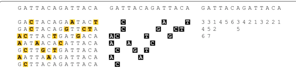
Consider a biallelic genetic site i with alleles {A,B} . Con-sider the vector h1,i, h2,i,. . .,hk,i ∈ {A,B}k of alleles of haplotypes j at site i. Label the allele A, B which occurs more frequently in this vector as the major allele 0, and the one which occurs less frequently as the minor allele 1. We then encode this vector by storing the value A or B of the major allele 0, and the indices j1,j2,. . . of the
haplo-types which take on allele value 1 at this site.
We will write φi for the subvector hj1,i,hj2,i,. . . of alleles
of haplotypes consisting of those haplotypes which pos-sess the minor allele 1 at site i. We will write |φi| for the
multiplicity of the minor allele. We call this vector φi the information content of the haplotype cohort H at the site
i.
Relation to the allele frequency spectrum
Our sparse representation of the haplotype reference panel benefits from the recent finding [9] that the dis-tribution over sites of minor allele frequencies is biased towards low frequencies.1
Clearly, the distribution of |φi| is precisely the allele
fre-quency spectrum. More formally,
Lemma 1 LetE[f](k)be the expected mean minor allele frequency forkgenotypes. Then
(6) E
1 n
n
i=1 |φi|
=E[f](k)
Corollary 1 If O(E[f]) <O(k) , then O(
i|φi|)
<O(nk)in expected value.
Dynamic reference panels
Adding or rewriting a haplotype is constant time per site per haplotype unless this edit changes which allele is the most frequent. It can be achieved by addition or removal or single entries from the row-sparse-column representa-tion, wherein, since our implementation does not require that the column indices be stored in order, these opera-tions can be made O(1) . This allows our algorithm to
extend to uses of the Li and Stephens model where one might want to dynamically edit the reference panel. The exception occurs when φi= k2—here it is not absolutely
necessary to keep the formalism that the indices stored actually be the minor allele.
Implementation
For biallelic sites, we store our φi ’s using a length-n vector
of length |φi| vectors containing the indices j of the
haplo-types hj∈φi and a length-n vector listing the major allele
at each site (see Fig. 1 panel iii) Random access by key i to iterators to the first elements of sets φi is O(1) and
itera-tion across these φi is linear in the size of φi . For
multial-lelic sites, the data structure uses slightly more space but has the same speed guarantees.
Generating these data structures takes O(nk) time but
is embarrassingly parallel in n. Our “*.slls” data structure doubles as a succinct haplotype index which could be dis-tributed instead of a large vcf record (though genotype likelihood compression is not accounted for). A vcf → slls
conversion tool is found in our github repository.
Efficient dynamic programming
We begin with the recurrence relation of the clas-sic forward algorithm applied to the Li and Stephens
model [1]. To establish our notation, recall that we
write pi[j] =P(xj,i,o1,. . .,oi|H), that we write µi(j)
as shorthand for p(oi|xj,i) and that we have initialized p1[j] =p(xj,1,o1|H)= µ1k(j) . For i>1 , we may then write:
We will reduce the number of summands in (8) and
reduce the number indices j for which (7) is evaluated. This will use the information content defined in "Sparse column representation of haplotype alleles" section.
(7) pi[j] =µi(j)
(1−kρi)pi−1[j] +ρiSi−1
(8) Si =
k
j=1 pi[j]
Lemma 2 The summation (8) is calculable using strictly fewer than k summands.
Proof Suppose first that µi(j)=µi for all j. Then
Now suppose that µi(j)=1−µi for some set of j. We
must then correct for these j. This gives us
The same argument holds when we reverse the roles of µi
and 1−µi . Therefore we can choose which calculation to
perform based on which has fewer summands. This gives us the following formula:
where
(9) Si=
k
j=1
pi[j] =µi k
j=1
(1−kρi)pi−1[j] +ρiSi−1
(10) =µi((1−kρi)Si−1+kρiSi−1)=µiSi−1
(11) Si=µiSi−1+
1−µi−µi 1−µi
jwhereµi(j)�=µi pi[j]
(12) Si=αSi−1+β
j∈φi pi[j]
(13) α=µi β =
1−2µi
1−µi ifφihave allele a
(14) α=1−µi β=
2µi−1 µi
ifφido not have allele a
We note another redundancy in our calculations. For the proper choices of µ′i,µ′′i among µi, 1−µi , the
recur-rence relations (7) are linear maps R→R
of which there are precisely two unique maps, fi
corre-sponding to the recurrence relations for those xj such that j∈φi , and Fi to those such that j∈/φi.
Lemma 3 If j∈/φiand j∈/φi−1 , thenSi can be calcu-lated without knowing pi−1[j]and pi[j] . If j∈/φi−1and
j′�=j , then pi[j′] can be calculated without knowing pi−1[j].
Proof Equation (12) lets us calculate Si−1
with-out knowing any pi−1[j] for any j∈/φi−1 . From Si−1
we also have fi and Fi . Therefore, we can calculate
pi[j′] =fi(pi−1[j′])or Fi(pi−1[j′]) without knowing pi−1[j]
provided that j′�=j . This then shows us that we can cal-culate pi[j′] for all j′∈φi without knowing any j such that
j∈/φi and j∈/φi−1 . Finally, the first statement follows
from another application of (12) (Fig. 2).
Corollary 2 The recurrences (8) and the minimum set of recurrences (7) needed to compute (8) can be evaluated inO(|φi|)time, assuming thatpi−1[j]have been computed
∀j∈φi.
We address the assumption on prior calculation of the necessary pi−1[j] ’s in "Lazy evaluation of dynamic pro-gramming rows" section.
Time complexity
Recall that we defined E[f](k) as the expected mean minor allele frequency in a sample of size k. Suppose that it is comparatively trivial to calculate the missing pi−1[j] (15) fi:x�−→µ′i(1−kρ)x+µ′iρSi−1
(16) Fi:x�−→µ′′i(1−kρ)x+µ′′iρSi−1
G A T T A C A G A T T A C A
G A C T A C A G A A T A C T
G A C T A C A G G T T C T A
A C T T A C T G A T G A C A
A A T A A C A C A T T A C A G C T T G C T G A T T A C A
A A T T A A A G A T T A C A G C T T A C A G A T T A C A
G A T T A C A G A T T A C A
G A C T A C A G A A T A C T
G A C T A C A G G T T C T A
A C T T A C T G A T G A C A
A A T A A C A C A T T A C A G C T T G C T G A T T A C A
A A T T A A A G A T T A C A G C T T A C A G A T T A C A
G A T T A C A G A T T A C A
3 3 1 4 5 6 3 4 2 1 3 2 2 1 4 5 2 5
6 7
Fig. 1 Information content of array of template haplotypes. (i) Reference panel {h1,. . .,h5} with mismatches to haplotype o shown in yellow. (ii)
values. Then by Corollary 2 the procedure in Eq. (12) has
expected time complexity O
i|φi|
=O
nE[f](k)
.
Lazy evaluation of dynamic programming rows
Corollary 2 was conditioned on the assumption that spe-cific forward probabilities had already been evaluated. We will describe a second algorithm which performs this task efficiently by avoiding performing any arithmetic which will prove unnecessary at future steps.2
Equivalence classes of longest major allele suffixes
Lemma 4 Suppose thathj∈/φℓ ∪ φℓ+1 ∪ . . . ∪ φi−1 . Then the dynamic programming matrix entries pℓ[j], pℓ+1[j], . . ., pi−1[j]need not be calculated in order
to calculateSℓ, Sℓ+1, . . ., Si−1.
Proof By repeated application of Lemma (3).
Corollary 3 Under the same assumption on j,
pℓ[j], pℓ+1[j], . . ., pi−1[j]need not be calculated in order
to calculateFℓ+1, . . ., Fi . This is easily seen by definition
ofFi.
Lemma 5 Suppose that pℓ−1[j] is known, and xj ∈/φℓ ∪ φℓ+1 ∪ . . . ∪ φi−1 . Thenpi−1[j]can be calcu-lated in the time which it takes tocalculateFi−1◦. . .◦Fℓ.
Proof pi−1[j] =Fi−1◦. . .◦Fℓ(pℓ−1[j])
It is immediately clear that calculating the pi[j] lends well
to lazy evaluation. Specifically, the xj∈/φi are data which
need not be evaluated yet at step i. Therefore, if we can aggregate the work of calculating these data at a later iter-ation of the algorithm, and only if needed then, we can potentially save a considerable amount of computation.
Definition 2 (Longest major allele suffix classes) Define
Eℓ→i−1=φℓ−1∩
i−1
ι=ℓφι
c
That is, let Eℓ→i−1 be the
class of all haplotypes whose sequence up to site i−1 shares the suffix from ℓ to i−1 inclusive consisting only of major alleles, but lacks any longer suffix composed only of major alleles.
Remark 1 Eℓ→i−1 is the set of all hj where pℓ−1[j] was
needed to calculate Sℓ−1 but no p(·)[j] has been needed to
calculate any S(·) since.
Note that for each i, the equivalence classes Eℓ→i−1
form a disjoint cover of the set of all haplotypes hj∈H.
Remark 2 ∀hj∈Eℓ→i−1 , pi−1[j] =Fi−1◦. . .◦Fℓ(pℓ−1[j])
Definition 3 Write Fa→b as shorthand for Fb◦. . .◦Fa.
The lazy evaluation algorithm
Our algorithm will aim to:
1. Never evaluate pi[j] explicitly unless hj∈φi.
2. Amortize the calculations pi[j] =fi◦Fi−1◦. . .
◦Fℓ(pℓ−1[j]) over all hj∈Eℓ→i−1.
3. Share the work of calculating subsequences of
com-positions of maps Fi−1◦. . .◦Fℓ with other
composi-tions of maps Fi′−1◦. . .◦Fℓ′ where ℓ′≤ℓ and i′≥i.
To accomplish these goals, at each iteration i, we main-tain the following auxiliary data. The meaning of these are clarified by reference to Figs. 3, 4 and 5.
1. The partition of all haplotypes hj∈H into
equiva-lence classes Eℓ→i−1 according to longest major allele
suffix of the truncated haplotype at i−1 . See
Defini-tion 2 and Fig. 3.
2. The tuples Tℓ=(Eℓ→i−1,Fℓ→m,m) of
equiva-lence classes Eℓ→i−1 stored with linear map
pre-fixes Fℓ→m=Fm◦. . .◦Fℓ of the map Fℓ→i−1 which
would be necessary to fully calculate pi[j] for the j
they contain, and the index m of the largest index in
this prefix. See Fig. 5.
3. The ordered sequence m1>m2> . . . , in reverse
order, of all distinct 1≤m≤i−1 such that m is
contained in some tuple. See Figs. 3, 5.
4. The maps Fmin{ℓ}→mmin, . . ., Fm2+1→m1, Fm1+1→i−1
which partition the longest prefix Fi−1◦. . .◦Fmin{ℓ}
into disjoint submaps at the indices m. See Fig. 3.
(i) (ii)
Fig. 2 Work done to calculate the sum of haplotype probabilities at a site for the conventional and our sublinear forward algorithm. Using the example that at site i, φi(oi)= {h3} , we illustrate the number
of arithmetic operations used in (i) the conventional O(nk) Li and Stephens HMM recurrence relations. ii Our procedure specified in Eq. (12). Black lines correspond to arithmetic operations; operations which cannot be parallelized over j are colored yellow
These are used to rapidly extend prefixes Fℓ→m into
prefixes Fℓ→i−1.
Finally, we will need the following ordering on tuples Tℓ to describe our algorithm:
Definition 4 Impose a partial ordering < on the
Tℓ=(Eℓ→i−1,Fℓ→m,m) by Tℓ<Tℓ′ iff m<m′ . See Fig. 4.
We are now ready to describe our lazy evaluation algo-rithm which evaluates pi[j] =fi◦Fℓ→i−1(pℓ−1[j])
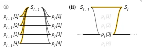
just-in-time while fulfilling the aims listed at the top of this section, by using the auxiliary state data specified above. Fig. 3 Longest major allele suffix classes, linear map compositions. Illustrations clarifying the meanings of the equivalence classes Eℓ→i−1 (left) and the maps Fa→b . Indices m are sites whose indices are b’s in stored maps of the form Fa→b
Fig. 4 Partial ordering of tuples of (equivalence class, linear map, index) used as state information in our algorithm. The ordering of the tuples Tℓ=(Eℓ→i−1,Fℓ→m,m) . Calculation of the depth d of an update which requires haplotypes contained in the equivalence classes defining the two
The algorithm is simple but requires keeping track of a number of intermediate indices. We suggest referring to the Figs. 3, 4 and 5 as a visual aid. We state it in six steps as follows.
Step 1: Identifying the tuples containing φ—O(φi)
time complexity
Identify the subset U(φ) of the tuples Tℓ for which there exists some hj∈φi such that hj∈Eℓ→i−1.
Step 2: Identifying the preparatory map suffix calcula-tions to be performed—O(φi) time complexity
Find the maximum depth d of any Tℓ∈U(φ)
with respect to the partial ordering above.
Equivalently, find the minimum m such that
Tℓ=(Eℓ→i−1,Fℓ→m,m)∈U(φ) . See Fig. 4.
Step 3: Performing preparatory map suffix calcula-tions—O(d) time complexity
1 O(d) : Let m1,. . .,md be the last d indices m in the
reverse ordered list of indices m1,m2,. . . . By
itera-tively composing the maps Fm1+1→i−1,Fm2+1→m1
which we have already stored, construct the
telescop-ing suffixes Fm1+1→i−1, Fm2+1→i−1,. . ., Fmd+1→i−1
needed to update the tuples (Eℓ→i−1,Fℓ→m,m) to
(Eℓ→i−1,Fℓ→i−1,i−1).
2 O(d) : For each m1≤mi ≤md , choose an
arbi-trary (Eℓ→i−1,Fℓ→mi,mi) and update it to
(Eℓ→i−1,Fℓ→i−1,i−1).
Fig. 5 Key steps involved in calculating pi[j] by delayed evaluation. An illustration of the manipulation of the tuple T2=(Eℓ→i−1,Fℓ→m,m) by the
lazy evaluation algorithm, and how it is used to calculate pi[j] from pℓ−1[j] just-in-time. In this case, we wish to calculate p6[2] . This is a member of the equivalence class E2→5 , since it hasn’t needed to be calculated since time 1. In step 4 of the algorithm, we therefore must update the whole
tuple T2 by post-composing the partially completed prefix F2→4 of the map F2→5 which we need using our already-calculated suffix map F5 . In step
Step 4: Performing the deferred calculations for the tuples containing hj∈φi—O(φi) time complexity
If not already done in Step 3.2, for every Tℓ∈U(φ) , extend its map element from (Eℓ→i−1,Fℓ→m,m) to
(Eℓ→i−1,Fℓ→i−1,i−1) in O(1) time using the maps
cal-culated in Step 3.1. See Fig. 5.
Step 5: Calculating pi[j] just-in-time—O(φi) time complexity
Note: The calculation of interest is performed here. Using the maps Fℓ→i−1 calculated in Step 3.2 or 4,
finally evaluate the value pi[j] =fi◦Fℓ→i−1(pℓ−1[j]) . See
Fig. 5.
Step 6: Updating our equivalence class/update map prefix tuple auxiliary data struc-tures—O(φi+d) time complexity
1. Create the new tuple (Ei→i,Fi→i = identity map ,i).
2. Remove the hj∈φi from their equivalence classes
Eℓ→i−1 and place them in the new equivalence class
Ei→i . If this empties the equivalence class in question,
delete its tuple. To maintain memory use bounded by
number of haplotypes, our implementation uses an object pool to store these tuples.
3. If an index mi no longer has any corresponding tuple,
delete it, and furthermore replace the stored maps
Fmi−1+1→mi and Fmi+1→mi+1 with a single map
Fmi−1+1→mi+1 . This step is added to reduce the upper
bound on the maximum possible number of composi-tions of maps which are performed in any given step.
The following two trivial lemmas allow us to bound d
by k such that the aggregate time complexity of the lazy evaluation algorithm cannot exceed O(nk) . Due to the
irregularity of the recursion pattern used by the algo-rithm, is likely not possible to calculate a closed-form
tight bound on
id , however, empirically it is
asymp-totically dominated by
iφi as shown in the results
which follow.
Lemma 6 The number of nonempty equivalence classes
Eℓ→i−1in existence at any iterationi of the algorithm is bounded by the number of haplotypesk.
Proof Trivial but worth noting.
Lemma 7 The number of unique indicesmin existence at any iterationiof the algorithm is bounded by the num-ber of nonempty equivalenceclassesEℓ→i−1.
Results Implementation
Our algorithm was implemented as a C++ library located at https ://githu b.com/yohei rosen /subli near-Li-Steph ens. Details of the lazy evaluation algorithm will be found there.
We also implemented the linear time forward
algo-rithm for the haploid Li and Stephens model in C++
as to evaluate it on identical footing. Profiling was per-formed using a single Intel Xeon X7560 core running at 2.3 GHz on a shared memory machine. Our reference
panels H were the phased haplotypes from the 1000
Genomes [10] phase 3 vcf records for chromosome 22
and subsamples thereof. Haplotypes o were randomly
generated simulated descendants.
Minor allele frequency distribution for the 1000 Genomes dataset
We found it informative to determine the allele frequency spectrum for the 1000 Genomes dataset which we will use in our performance analyses. We simulated
haplo-types o of 1,000,000 bp length on chromosome 22 and
recorded the sizes of the sets φi(oi) for k=5008 . These
data produced a mean |φi(oi)| of 59.9, which is 1.2% of the
size of k. We have plotted the distribution of |φi(oi)| which
we observed from this experiment in (Fig. 6). It is skewed toward low frequencies; the minor allele is unique at 71% of sites, and it is below 1% frequency at 92% of sites.
Comparison of our algorithm with the linear time forward algorithm
In order to compare the dependence of our algorithm’s runtime on haplotype panel size k against that of the standard linear LS forward algorithm, we measured the CPU time per genetic site of both across a range of haplotype panel sizes from 30 to 5008. This analysis was achieved as briefly described above. Haplotype panels spanning the range of sizes from 30 to 5008 haplotypes were subsampled from the 1000 Genomes phase 3 vcf records and loaded into memory in both uncompressed and our column-sparse-row format. Random sequences were sampled using a copying model with mutation and recombination, and the performance of the classical for-ward algorithm was run back to back with our algorithm for the same random sequence and same subsampled haplotype panel. Each set of runs was performed in tripli-cate to reduce stochastic error.
Figure 7 shows this comparison. Observed time
com-plexity of our algorithm was O(k0.35) as calculated from
the slope of the line of best fit to a log–log plot of time per site versus haplotype panel size.
is 37 μs for our algorithm and 1308 μs for the linear LS algorithm. For the forthcoming 100,000 Genomes Pro-ject, these numbers can be extrapolated to 251 μs for our algorithm and 260,760 μs for the linear LS algorithm.
Lazy evaluation of dynamic programming rows
We also measured the time which our algorithm spent within the d-dependent portion of the lazy evaluation subalgorithm. In the average case, the time complexity of our lazy evaluation subalgorithm does not contribute to the overall algebraic time complexity of the algorithm (Fig. 8, right). The lazy evaluation runtime also contrib-utes minimally to the total actual runtime of our algo-rithm (Fig. 8, left).
Sparse haplotype encoding Generating our sparse vectors
We generated the haplotype panel data structures from "Sparse representation of haplotypes" section using the
vcf-encoding tool vcf2slls which we provide. We
built indices with multiallelic sites, which increases their time and memory profile relative to the results in "Minor allele frequency distribution for the 1000 Genomes data-set" section but allows direct comparison to vcf records. Encoding of chromosome 22 was completed in 38 min on a single CPU core. Use of M CPU cores will reduce runt-ime proportional to M.
Size of sparse haplotype index
In uncompressed form, our whole genome *.slls
index for chromosome 22 of the 1000 genomes dataset was 285 MB in size versus 11 GB for the vcf record using uint16_t’s to encode haplotype ranks. When com-pressed with gzip, the same index was 67 MB in size ver-sus 205 MB for the vcf record.
In the interest of speed (both for our algorithm and the
O(nk) algorithm) our experiments loaded entire
chromo-some sparse matrices into memory and stored haplotype Fig. 6 Biallelic site minor allele frequency distribution from 1000 Genomes chromosome 22. Note that the distribution is skewed away from the 1
f distribution classically theorized. The data used are the genotypes of the 1000 Genomes Phase 3 VCF, with minor alleles at multiallelic sites
combined
indices as uint64_t’s. This requires on the order of 1 GB memory for chromosome 22. For long chromosomes or larger reference panels on low memory machines, the algorithm can operate by streaming sequential chunks of the reference panel.
Discussions and Conclusion
To the best of our knowledge, ours is the first forward algorithm for any haplotype model to attain sublinear time complexity with respect to reference panel size. Our algorithms could be incorporated into haplotype infer-ence strategies by interfacing with our C++ library. This opens the potential for tools which are tractable on hap-lotype reference panels at the scale of current 100,000 to 1,000,000+ sample sequencing projects.
Applications which use individual forward probabilities
Our algorithm attains its runtime specifically for the problem of calculating the single overall probability P(o|H,ρ,µ) and does not compute all nk forward
prob-abilities. We can prove that if m many specific forward probabilities are also required as output, and if the time complexity of our algorithm is O(
i|φi|) , then the time
complexity of the algorithm which also returns the m for-ward probabilities is O(
i|φi| +m).
In general, haplotype phasing or genotype imputation tools use stochastic traceback or other similar sampling algorithms. The standard algorithm for stochastic trace-back samples states from the full posterior distribution and therefore requires all forward probabilities. The algo-rithm output and lower bound of its speed is therefore
O(nk) . The same is true for many applications of the
for-ward–backward algorithm.
There are two possible approaches which might allow
runtime sublinear in k for these applications. Using
stochastic traceback as an example, first is to devise an
O(f(m)) sampling algorithm which uses m=g(k)
for-ward probabilities such that O(f ◦g(k)) <O(k) . The
sec-ond is to succinctly represent forward probabilities such that nested sums of the nk forward probabilities can be queried from O(φ) <O(nk) data. This should be
pos-sible, perhaps using the positional Burrows–Wheeler transform [11] as in [8], since we have already devised a forward algorithm with this property for a different model in [12].
Generalizability of algorithm
The optimizations which we have made are not strictly specific to the monoploid Li and Stephens algorithm. Necessary conditions for our reduction in the time com-plexity of the recurrence relations are
Condition 1 The number of distinct transition probabili-ties is constant with respect to number of statesk.
Condition 2 The number of distinct emission probabili-ties is constant with respect to number of statesk.
Favourable conditions for efficient time complexity of the lazy evaluation algorithm are
Condition 1 The number of unique update maps added per step is constant with respect to number of statesk.
Condition 2 The update map extension operation is composition of functions of a class where composition is constant-time with respect to number of statesk.
The reduction in time complexity of the recurrence relations depends on the Markov property, however we hypothesize that the delayed evaluation needs only the semi-Markov property.
Other haplotype forward algorithms
Our optimizations are of immediate interest for other haplotype copying models. The following related algo-rithms have been explored without implementation.
Example 1 (Diploid Li and Stephens) We have yet to implement this model but expect average runtime at least subquadratic in reference panel size k. We build on the statement of the model and its optimizations in [13]. We have found the following recurrences which we believe will work when combined with a system of lazy evalua-tion algorithms:
Lemma 8 The diploid Li and Stephens HMM may be expressed using recurrences of the form
which use on the intermediate sums defined as
whereα(·),β(·),γ(·)depend only on the diploid genotypeoi.
Implementing and verifying the runtime of this exten-sion of our algorithm will be among our next steps.
Example 2 (Multipopulation Li and Stephens) [14] We maintain separate sparse haplotype panel representations φiA(oi) and φiB(oi) and separate lazy evaluation mecha-nisms for the two populations A and B. Expected runtime guarantees are similar.
This model, and versions for >2 populations, will be
important in large sequencing cohorts (such as NHLBI TOPMed) where assuming a single related population is unrealistic.
(17)
pi[j1,j2] =αppi−1[j1,j2] +βp(Si−1(j1)+Si−1(j2))+γpSi−1
(18)
Si:=αcSi−1+βc
j∈φi
Si−1(j)
+γc
(j1,j2)∈φi2
pi−1[j1,j2] O(|φi|2)
(19)
Si(j):=αcSi−1+βcSi−1(j)
+γc
j2∈φi
pi−1[j,j2] forO(k|φi|)manyj
Example 3 (More detailed mutation model) It may also be desirable to model distinct mutation probabilities for different pairs of alleles at multiallelic sites. Runtime is worse than the biallelic model but remains average case sublinear.
Example 4 (Sequence graph Li and Stephens analogue) In [12] we described a hidden Markov model for a haplo-type-copying with recombination but not mutation in the context of sequence graphs. Assuming we can decom-pose our graph into nested sites then we can achieve a fast forward algorithm with mutation. An analogue of our row-sparse-column matrix compression for sequence graphs is being actively developed within our research group.
While a haplotype HMM forward algorithm alone might have niche applications in bioinformatics, we expect that our techniques are generalizable to speed-ing up other forward algorithm-type sequence analysis algorithms.
Authors’ contributions
YR designed and prototyped the algorithm described in this article and performed its speed benchmarking. BP conceived of the theoretical need for such an algorithm and designed its integration into ongoing variant calling research. Both authors read and approved the final manuscript.
Author details
1 UCSC Genomics Institute, 1156 High St, Santa Cruz, CA 95064, USA. 2 NYU School of Medicine, 550 First Ave, New York, NY 10016, USA.
Acknowledgements
This work was supported by the National Human Genome Research Institute of the National Institutes of Health under Award Number 5U54HG007990, the National Heart, Lung, and Blood Institute of the National Institutes of Health under Award Number 1U01HL137183-01, and grants from the W.M. Keck foun-dation and the Simons Founfoun-dation. We would like to thank Jordan Eizenga for his helpful discussions throughout the development of this work.
Competing interests
The authors declare that they have no competing interests.
Availability of data and materials
The dataset used as template haplotypes for the performance profiling during the current study are available in the 1000 Genomes Phase 3 variant call release, ftp://ftp.1000g enome s.ebi.ac.uk/vol1/ftp/relea se/20130 502/ The runtime data produced during the current study are available from the corre-sponding author on reasonable request. The randomly generated subsampled haplotype cohorts and haplotypes used in these analyses persisted only in memory and were not saved to disk due to their immense aggregate size.
Publisher’s Note
Springer Nature remains neutral with regard to jurisdictional claims in pub-lished maps and institutional affiliations.
•fast, convenient online submission •
thorough peer review by experienced researchers in your field • rapid publication on acceptance
• support for research data, including large and complex data types •
gold Open Access which fosters wider collaboration and increased citations maximum visibility for your research: over 100M website views per year •
At BMC, research is always in progress.
Learn more biomedcentral.com/submissions
Ready to submit your research? Choose BMC and benefit from: References
1. Li N, Stephens M. Modeling linkage disequilibrium and identifying recombination hotspots using single-nucleotide polymorphism data. Genetics. 2003;165(4):2213–33.
2. Kingman JFC. The coalescent. Stoch Process Appl. 1982;13(3):235–48. 3. Loh P-R, Danecek P, Palamara PF, Fuchsberger C, Reshef YA, Finucane HK, Schoenherr S, Forer L, McCarthy S, Abecasis GR. Reference-based phasing using the haplotype reference consortium panel. Nat Genet. 2016;48(11):1443.
4. Browning BL, Browning SR. A unified approach to genotype imputation and haplotype-phase inference for large data sets of trios and unrelated individuals. Am J Human Genet. 2009;84(2):210–23.
5. Williams AL, Patterson N, Glessner J, Hakonarson H, Reich D. Phas-ing of many thousands of genotyped samples. Am J Human Genet. 2012;91(2):238–51.
6. Delaneau O, Zagury J-F, Marchini J. Improved whole-chromosome phasing for disease and population genetic studies. Nat Methods. 2013;10(1):5.
7. O’Connell J, Sharp K, Shrine N, Wain L, Hall I, Tobin M, Zagury J-F, Dela-neau O, Marchini J. Haplotype estimation for biobank-scale data sets. Nat Genet. 2016;48(7):817.
8. Lunter G. Fast haplotype matching in very large cohorts using the li and stephens model. bioRxiv 2016. https ://doi.org/10.1101/04828 0. https :// www.biorx iv.org/conte nt/early /2016/04/12/04828 0.full.pdf.
9. Keinan A, Clark AG. Recent explosive human population growth has resulted in an excess of rare genetic variants. Science. 2012;336(6082):740–3.
10. Consortium GP, et al. A global reference for human genetic variation. Nature. 2015;526(7571):68.
11. Durbin R. Efficient haplotype matching and storage using the positional Burrows–Wheeler transform (PBWT). Bioinformatics. 2014;30(9):1266–72. 12. Rosen Y, Eizenga J, Paten B. Modelling haplotypes with respect to
refer-ence cohort variation graphs. Bioinformatics. 2017;33(14):118–23. 13. Li Y, Willer CJ, Ding J, Scheet P, Abecasis GR. Mach: using sequence and
genotype data to estimate haplotypes and unobserved genotypes. Genet Epidemiol. 2010;34(8):816–34.

![Fig. 5 Key steps involved in calculating lazy evaluation algorithm, and how it is used to calculate tuple pi[j] by delayed evaluation](https://thumb-us.123doks.com/thumbv2/123dok_us/334418.1525912/7.595.61.540.87.461/steps-involved-calculating-evaluation-algorithm-calculate-delayed-evaluation.webp)


