O R I G I N A L A R T I C L E
Open Access
Applying Bayesian model averaging for uncertainty
estimation of input data in energy modelling
Monika Culka
Abstract
Background:Energy scenarios that are used for policy advice have ecological and social impact on society. Policy measures that are based on modelling exercises may lead to far reaching financial and ecological consequences. The purpose of this study is to raise awareness that energy modelling results are accompanied with uncertainties that should be addressed explicitly.
Methods:With view to existing approaches of uncertainty assessment in energy economics and climate science, relevant requirements for an uncertainty assessment are defined. An uncertainty assessment should be explicit, independent of the assessor’s expertise, applicable to different models, including subjective quantitative and statistical quantitative aspects, intuitively understandable and be reproducible. Bayesian model averaging for input variables of energy models is discussed as method that satisfies these requirements. A definition of uncertainty based on posterior model probabilities of input variables to energy models is presented.
Results:The main findings are that (1) expert elicitation as predominant assessment method does not satisfy all requirements, (2) Bayesian model averaging for input variable modelling meets the requirements and allows evaluating a vast amount of potentially relevant influences on input variables and (3) posterior model probabilities of input variable models can be translated in uncertainty associated with the input variable.
Conclusions:An uncertainty assessment of energy scenarios is relevant if policy measures are (partially) based on modelling exercises. Potential implications of these findings include that energy scenarios could be associated with uncertainty that is presently neither assessed explicitly nor communicated adequately.
Keywords:Uncertainty; Energy modelling; Assessment methods; Bayesian model averaging
Background
Energy scenarios are quantitative or qualitative output from mathematic modelsa of the energy system, or, systematic, consistent thinking in qualitative terms about the energy system. Quantitative energy models can be classified as top-down models, typically macro-economic models with focus on energy economics and bottom-up models, typic-ally technology oriented process-based models. Different mathematical descriptions of the target system are possible, such as general equilibrium models (e.g. E3ME [1]), linear programs (e.g. TIMES [2]), stochastic models (e.g. [3], espe-cially [4]) or mixed complementary problems (e.g. [5]). If an energy model has an objective function to be minimised or maximised, it is an optimisation model. Opposed to these, simulation models simulate consequences over time
of key assumptions. Frequently used terms in that context are business as usual scenario or reference scenario. An energy scenario can describe both, key assumptions about relevant input variables in energy economics, and the result of a model run, the model output. In this text, the term energy scenario refers to the results of quantitative models. Amongst the most important input variables, also called key assumptions or assumption framework, are for example shares of specific electricity generation capacities, popula-tion growth assumppopula-tions, fuel price assumppopula-tions or gross domestic product assumptions. These key assumptions can be varied to produce alternative scenarios that can be assessed quantitatively by means of energy models or qualitatively in different storylines. The choice which key assumptions are considered in a study strongly depends on the aim of the research and is often coupled to specific questions regarding energy futures or political
Correspondence:[email protected]
KIT Institute of Philosophy, Kaiserstr.12, Karlsruhe 76128, Germany
considerations cf. [6,7]. One of the main aims of such energy scenarios are statements about the future, be it possible, probable, normative or deterministic statements. These statements may serve for political advice, or are the basis for (energy-) political decision making. Examples to illustrate this function are the Energiekonzept der Bundesregierung [8] in Germany that is at least inspired -by a modelling exercise, or, on a European level, the Energy Roadmap 2050 [9] that refers to a modelling exercise, detailed in part 2/2 of their publication.
The scenario report for the Energiekonzept introduces its findings with a clarification on what energy scenarios, as described in the report, are meant to be: ‘Scenarios describe possible futures. They do not claim to represent the most likely development from today’s perspective. […] Depending on the definition of relevant parameters (‘Eckpunkte’), next to the derived scenarios, many other pathways in the future of the German energy supply are possible that are not under scrutiny in this work’[10].
So, what discerns such a possibilistic statement (an energy scenario) from any other possibilistic energy scenario that, admittedly, may serve the same purpose of fulfilling the German energy supply? And if there is no difference, of what profit is the modelling exercise altogether? One answer can be found in the document, the developed target scenarios comprise consistent path-ways of long-term energy economic developments [10].
The question arises, what consistent in this context means. Consistent with expectations about the future, consistent with past evidence, consistent with the math-ematical model framework or consistent in a rather abstract sense that there are no contradictions in the energy scenarios. However interpreted, the question remains, what additional value, with respect to any other possible pathway, does a model-based pathway into the German energy future provide? Consistency, in the broadest sense could be understood in and by itselfaspossibility; for, if a statement is self-contradictory, it is not possible. Hence, consistency is no unique charac-teristic ofpossiblemodel-based statements. However, it is possible that some energy scenarios are not even consistent in a non-contradictory sense. Weimer-Jehle has developed a systematic approach to ensure that as-sumption preselection and associated effects on society, economy and environment are consistent and evaluated in a transparent way [11]. If such a transparent approach in the phase of key assumption selection or scenario con-struction is not provided, it remains at least questionable, if energy scenarios are not self-contradictory.
An added value could be derived, if model-based energy scenarios were contrasted to other possible scenarios, particularly, if an uncertainty assessment was carried out for the energy scenario. In the case of a quantitative uncertainty assessment, the possibility of comparing
different scenarios with respect to their adherent uncer-tainty could indicate to what extent and in what respect the scenario can be discerned from other scenarios. An energy scenario that is possible begs the question how possible it is, given key assumptions about the future. The question is thus, how uncertain is an energy scenario?
The main objective of this text is a discussion which requirements an uncertainty assessment should fulfil. Based on these requirements, a method, Bayesian model aver-aging (BMA) is debated as possible candidate to satisfy them. The main arguments are that an energy modelling exercise that is enriched with an uncertainty assessment which satisfies the requirements is (1) comprehensible in terms of its associated uncertainty and (2) should contrib-ute to a complete understanding of energy scenarios, espe-cially if they are used in decision support.
Uncertainties in energy scenarios can have different sources and can be of different kinds. Walker et al. have presented a concise summary of existent uncertainty of model-based energy scenarios, based on the location, level and nature of the uncertainty [12]. According to them, generic locations can be context, model uncertainty, inputs, parameter and outcome. The uncertainty estimation method discussed in this text, BMA for input variables to energy models, can assess uncertainty in the location input and parameter uncertainty, and, to an extent, context uncertainty that concerns the modelled boundaries of the system. The presented method does not aim to evaluate error propagation within a specific energy model. Walker describes the level of uncertainty in terms of determinism, statistical uncertainty, scenario uncertainty, recognised ignorance and indeterminacy, i.e. total ignorance. BMA for input variables to energy models represents uncer-tainty based on probabilistic assessment and hence can also range from certainty to total ignorance. However, the use of statistical data renders the assessment itself prone to statistical uncertainty. Finally, Walker et al. describe the nature of uncertainty as epistemic uncertainty or variabil-ity where epistemic uncertainty is due to the imperfection of our knowledge and variability refers to inherent vari-ability, especially present in human and natural systems. The BMA approach can evaluate both natures of uncer-tainty in statistical terms. If input variables to energy models are exposed to variability, data fit of model results with respect to statistical data will indicate that exposure.
exposed to variability such as electricity generation modelling based on wind or solar cf. [15,16]. Epistemic uncertainty is less naturally defined in a probabilistic framework, and hence, one of the objectives of uncer-tainty quantification is the reformulation of epistemic uncertainty as variability [17]. If epistemic uncertainty is contained in the energy model, the model results are likely to be more uncertain than the input variables. The BMA approach accounts for that by establishing a lower bound of uncertainty.
Recent evaluations have investigated the nature of energy scenarios and their limitations in terms of legit-imate inference from model output [6]. In contrast to a vivid discussion of model quality and legitimate infer-ence, as can be observed in climate modelling [18-21], energy models have not invoked a similar discussion. Whilst climate modelling developed a framework for the treatment and communication of uncertainties [22-24], energy models and resulting scenarios lack such a system-atic approach for uncertainty qualification (or quantifica-tion). However, investigating uncertainties in models is necessary for quality assessment of model results and reliability of results, especially if such results figure in policy advice.
The next chapter will investigate existing uncertainty assessments in energy modelling and focus on the strengths and weaknesses of those. From these considerations, gen-eral requirements that an uncertainty assessment for energy modelling should satisfy are retrieved. In the following sec-tion, presently applied methods for uncertainty evaluation are discussed, including expert elicitation, robustness ana-lysis, model fit, variety of evidence and standard statistical analysis. As research regarding uncertainty evaluation for energy models is not yet as advanced as for example in cli-mate science, a substantial part of discussion is based on examples of other disciplines, especially climate science. The next two sections firstly address critique on Bayesian approaches and present the uncertainty assessment based on BMA for input variables of energy models. The last sec-tion summarises results and discusses the method critically.
Existing uncertainty assessments in energy modelling
Data of already existing publications are compared with the results of this work, such that an evaluation of exist-ing approaches to uncertainty assessment in the context of energy economics is examined on the basis of two examples.
Walker et al. [12] have investigated energy model-related uncertainties with respect to their nature and occurrence. Their definition of uncertainty being ‘any departure from the unachievable ideal of complete determinism’, allows for a conceptual investigation of all relevant uncertainties, by defined categories, reaching from determinism to total ig-norance. The provided tool, an uncertainty matrix, should
be used to identify model outcome uncertainty according to their level and nature. It is not clear in what terms the matrix should be evaluated, yes/no, much/little, or, in a numeric scale that is not provided. This approach allows for an illustrative representation of uncertainties involved in modelling. However, the method seems to end with a delicate categorization rather than with a valuable assess-ment. Indeed, awareness of the location, level and nature of uncertainty is important information; nonetheless, the method does not provide insight into how the uncertainty should be assessed or into what way uncertainty of, for example, recognised ignorance in the location model structure bears on the uncertainty of model outcomes.
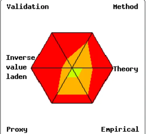
The second example of an assessment is the numeral unit spread assessment pedigree (NUSAP) method to assess qualitative and quantitative uncertainties in the targets image energy model regional (TIMER) energy model, part of RIVMs IMAGE model [25]. Firstly, by means of a comprehensive checklist for model quality assurance, key loci and sorts of uncertainties in the TIMER modelling process are identified. Model struc-ture uncertainties were analysed by a meta-analysis of similarities and differences of six energy models. A sensitivity analysis for model parameters in terms of magnitude of influence has been carried out. A NUSAP expert elicitation workshop has systematically assessed those parameters in the following dimensions: proxy, em-pirical basis, theoretical understanding, methodological rigour and validation. And finally, a diagnostic diagram is produced [25].
This evaluation provides interesting insight in the TIMER model, the uncertainties associated with the modelling process and the model results. However, there is some critique that relates to the applicability and required expert knowledge for such an assessment. Firstly, the method is rather model-specific. Secondly, the method relies mainly on expert elicitation for both experts in modelling and energy economics. Experts in modelling are likely to be experts for especially the model they work with. Large and complex models tend to require long periods of vocational adjustment before a model is fully understood. And due to intellectual property considerations, some models cannot be assessed by ‘foreign’ modellers. Another critical remark considers the output of the assessment. The diagnostic diagram, as presented in section 6.8 of document [25], is difficult to understand. The diagnostic diagram is based on the results of expert elicitation.
representing the dimensions of evaluation, namely, valid-ation, method, theory, empirical, proxy and inverse laden value. The green kite is spanned up by the minimum scores in each group for each pedigree criterion; the orange kite is spanned up by the maximum scores. The orange band between the green kite and the red area represents expert disagreement on the pedigree scores for that variable. In some cases, the picture was strongly influenced by a single deviating low score given by one of the six experts. In those cases, the light green kite
shows what the green kite would look like if that outlier would have been omitted. The 0 is in the center of the diagram and the 4 is on each corner. Note that, the scores for value ladenness have been inverted compared to what was filled in on the cards: a 4 on card was entered as a 0 in the diagram and a 0 on the card as a 4 in the diagram.
These three evaluationsallrepresent the uncertainty as-sociated with the learning rates of nuclear power produc-tion. There are several interpretations possible: either, the dissent in the expert groups indicates that the experts do not dispose of deep understanding of the questionc.
Or, one expert group is correct and the others are wrong. Or, the limited number of experts does not allow for the results to converge to an unambiguous assessment result. Or, the strong dissent indicates that uncertainty is high. This last reading is not without further ado more justified than any of the other readings. Yet, it is theonly one that actually assesses the uncertainty of the parameter in question. This example illustrates the necessity of an inter-subjective requirement in an assessment method. An inter-subjective assessment method would render the result of an uncertainty assessment less dependent on the specific individuals that carry out the analysis. If an assessment is based on expert elicitation and possible interpretations of dissent (and consent) are not explicit, the method itself contributes to uncertainty. For then, the uncertainty of the assessment method itselfandthe uncertainty of the model assessed are present, and it can be difficult to cleave them apart. It is necessary to stress that expert elicitation is an important tool. However, due to practical limitationsd, issues of the method in and
Figure 1NUSAP kite diagram for learning rates: a. Nuclear of group A.
Figure 2NUSAP kite diagram for learning rates: a. Nuclear of group B.
by itself, such as convergence in findings and trustworthi-ness of findings, need to be addressed and evaluated.
Based on these examples and general desirables for an uncertainty assessment, a list of requirements of an uncertainty assessment for energy scenarios can be formu-lated. The six following requirements are not exhaustive; other possibly relevant virtues could be imagined as requirements for uncertainty quantification are context dependent. The presented aspects are inspired by existing approaches and desirables with respect to methodology and practical aspects in energy economics and climate science. An uncertainty assessment should
1) give a clear indication how reliable the findings are (uncertainty assessment)
2) be applicable independent of assessor’s expertise (inter-subjectivity)
3) be applicable to different models (comparability of results)
4) incorporate qualitative and quantitative aspects (complete representation)
5) be intuitively understandable and straightforward to communicate (scale requirements)
6) be reproducible and unambiguous.
A clear indication of the reliability of findings (require-ment 1) can be achieved by quantitative methods rather than qualitative methods. Classical uncertainty quantifi-cation methods include, but are not limited to, both Frequentist and Bayesian statistical analysis, stochastic models, sensitivity analysis, or Monte Carlo methods [17,27]. Which quantification method is used strongly depends on the target system under scrutiny, the model representation of that system and the aspired precise-ness of the uncertainty quantification. Inter-subjectivity (requirement 2) can be interpreted as a maximisation of objectiveness in the assessment process. However, the incorporation of both quantitative and qualitative aspects (requirement 4), does implicitly demand subjective characteristics, for qualitative assessment methods demand subjective evaluation and understanding. The requirement of intuitive comprehensibility (requirement 5) should allow the recipient of such assessments an interpret-ation without tedious lecture of explanatory notes. And finally, reproducibility and unambiguousness (requirement 6) should minimise misunderstandings and increase confi-dence in the evaluation by the recipiente. The expected scientific progress by the proposed BMA method of un-certainty assessment in the context of energy economics can be summarised as follows
The assessment method does not solely rely on
expert elicitation, although valuable subjective expert knowledge can be included.
BMA could provide a versatile tool for the
assessment of complex interrelated statistical data.
Requirements that should be satisfied by an
uncertainty measurement method are met.
An explicit uncertainty assessment of energy scenarios that satisfies these requirements would increase trans-parency of assumption uncertainty and thus model results. The aims of the text are to present a methodology, BMA for input variables of energy models, that satisfies these requirements and to infer quantitative uncertainty estima-tions from input parameters to energy models. Recipients of energy scenarios could gain a better understanding regarding the uncertainty of model results (i.e. energy scenarios) what might impact their function as decision support or basis for decision, especially if energy scenarios are used for policy advice, leading to far reaching eco-logical, financial and societal consequences.
Methods
Quantitative methods versus qualitative methods for uncertainty assessments
In the quest of an appropriate uncertainty assessment for energy scenarios, climate science may provide a suitable starting point as the uncertainty assessment discussion in climate sciences is more advanced than in energy economics.
The Intergovernmental Panel on Climate Change (IPCC) has developed over years guidelines for a consistent treat-ment of uncertainties associated with climate modelling results. For the current report, the fifth assessment report, the published guidelines incorporate many of former critics on the initial uncertainty assessments and critically analyses uncertainty assessments of earlier reports [28]. The guide-lines of the assessment report 5 (AR5) specify two metrics for the communication of the degree of certainty in key findings:
Confidence in the validity of a finding, based on the
type, amount, quality and consistency of evidence (e.g. mechanistic understanding, theory, data, models, expert judgement) and the degree of agreement. Confidence is expressed qualitatively.
Quantified measures of uncertainty in a finding
expressed probabilistically (based on statistical analysis of observations or model results, or expert judgement) [23].
of uncertainty is recommended to be applied only in cases with high or very high confidence [29]f.
The IPCC uncertainty assessment thus relies on both, qualitative and quantitative ways to describe reliability of findings. Apparently, if quantitative assessments are applicable, they should be used preferable to qualitative assessment. Qualitative uncertainty assessment is applied in cases of deep uncertaintyg, where uncertainty cannot be quantified. Qualitative uncertainty assessment faces several challenges. The problem of linguistic ambiguity seems to be the predominant problem when uncertainty is qualitatively assessed. In the guidance, note the level of confidence is defined using five qualifiers: very low, low, medium, high and very high [23]. It synthesises the author teams’judgments about the validity of findings as determined through evaluation of evidence and agree-ment. It is arguable if there is a common understanding of such categories amongst individuals and hence, the question arises, whether the evaluation of agreement actually depicts the uncertainty of the finding in question or rather the ambiguity in understanding of the term used. Also, there is no clear indication how much agreement is necessary for the affiliation to a certain categoryh. And, finally, it is unclear in which way agreement can be associated with high confidence and in turn with uncer-tainty (judgments about the validity of findings). One interpretation could be that high confidence (inter alia based on high agreement) means low uncertainty; how-ever, this could not hold true in cases where agreement is high that the level of uncertainty is high for a finding (e.g. due to the stochastic nature of a process). More-over, this reading also faces the criticism that it is thinkable that even with high agreement, the finding is not at all certain, and all assessors could collectively be wrong in their valuation. The other reading, that high confidence means high uncertainty, next to being counter-intuitive, does not reflect that agreement sometimes does give an indication for the truth of a finding.
Qualitative assessment methods, even if normalised to summary terms (IPCC) seem to intrinsically depend on not only a subjective comprehension of summary terms but also subjective opinion of the assessor. This can be advantageous or disadvantageous, depending on the expert-ise of the assessor and the communication of relevant infor-mation that influenced the assessment. In any case, such assessment methods lack the important property of gener-ating reproducible assessments. If a different group of experts assessed the results, the uncertainty assessment of a specific finding might turn out to be significantly different, even if a sound reasoning underpins the assessment. As Krueger et al. point out, expert opinion in modelling will benefit from formal, systematic and transparent procedures [30]. Inter-subjective reproducibility is a necessity if a find-ing is called robust. A qualitative assessment is likely to be
not as efficient in evaluating robustness as a quantitative, standardised assessment, given the problem of linguistic ambiguity and subjectivity of the assessment method. A quantitative approach that uses a method that can be standardised and applied independent of the expertise of the assessor would presumably yield higher agreement.
However, qualitative uncertainty assessments have the important benefit of putting findings into perspective of the state of art of modelling and the present knowledge about processes and/or assumptions. If a finding is based on limited knowledge, it cannot represent a certain statement and has to be supplemented with information regarding the validity of findings.
Quantitative assessment methods often face the critique of being perceived with more precision than justified [31,32], especially [33] when he discusses Nowotny’s per-spective. This could be the case where probability density functions (pdfs) can be produced but are themselves based on uncertain input. In such cases, communication (quali-tatively or quanti(quali-tatively) of the uncertainty related to the pdfs is necessary. An advantage of quantitative methods is an unambiguous representation. The intuitive understand-ing, even in the simplest form, for example, a scale from one to ten, ten representing high uncertainty, might allow the recipient of such an assessment a clear understanding. This is, indeed, not unproblematic. For one, there is an intrinsic assumption that must be clarified if not true, which is that the scale units are uniform in sizei or a logarithmic scale. Even more intuitively understandable appears to be a probabilistic statement. However, re-garding the perception of probabilistic uncertainty assessments, Patt et al. report that changes of equal magnitude in assessed probabilities can have different effects in decision-making experiments. For example, a change of 10 percentage points from 90% to 100% impacts choices of test persons differently than a change from 50% to 60% [34]. Nonetheless, a probabilistic statement is in itself less susceptible to interpretational errors or misunderstandings than a qualitative statement that uses -again - words for interpretation that might be ambiguous.
analysed by ignorance aversion. Indeed, quantification, or for that matter qualification to summary terms, can result in a loss of detail and reasoning. It is not totally clear how bias can be created through such a process. However, it is the very task of an uncertainty assessment to transform in-formation of various kinds (quantitative, qualitative, narra-tive, implicit assumptions, etc.) into a form that can be understood without the profound expertise that is neces-sary to accomplish the uncertainty assessment itself.
The question whether a quantitative assessment method is preferable to a qualitative assessment method cannot be answered purely by evaluating the respective (dis-) advan-tages. There are practical limitations that may render a quantitative assessment impossible. However, for the development of an uncertainty assessment in the context of energy economics, relevant differences to climate science prevail that might justify the preferable use of quantitative methods.
Climate science and energy economics
The discussion concerning confirmation of climate models may serve as orientation, and energy model evaluation could profit from these considerations. Lloyd [20] con-cludes that climate models should not be judged primarily or solely on the basis of what they are weak at. This is an important aspect to remember when evaluating energy models as well. Generally, her approach to confirmation ‘takes it as a matter of degree; models can accrue credit and trustworthiness upon being supported by empirical evidence as well as by theoretical derivation’. Lloyd illus-trates the strengths in terms of confirmation asmodel fit, variety of evidence,independent support for aspectsof the models and robustness for climate models. These con-cepts, bearing on the reliability of models, can be applied to energy models as well.
Model fit
Model fit refers to the ability of model results to repre-sent data that can be observed empirically, possibly ex post. Unfortunately, energy models have a rather poor history of model fit [36,37]. Analysis of the main reasons for deviations of model results to evidence are sum-marised as:
unanticipated strong political decisions such as
closing of mines in the UK, feed-in tariffs in Germany and world climate change concerns;
unexpected energy requirements, like the transport
behaviour and the rush for gas;
definition and availability of statistical data [36].
The main difference when comparing climate models with energy models is that energy models represent and simulate a well-understood system with mainly economic
drivers. In contrast, climate modelling has its challenges in representing chaotic systems with at least partially little understood causal relationships and magnitudes of impact of system components. It was, at least in principle, pos-sible to know today with sufficient accuracy how the energy system will look like in a given point of time in the future. The problem is that many interests must be met and decisions not tend to be of durable nature as political, environmental or economic circumstances change. This is one reason why energy roadmaps, energy strategies and energy programs on a political level are important. These commitments to a specific system state in future allow for energy modellers to accordingly define constraints in models and consequently investigate - using models - dif-ferent paths to meet the desiderata. Results of such model simulations may be cost-effective, environmental-friendly, socially accepted or other (possibly optimised) system development paths. The reason why model fit of energy models yields a poor record in the past hence is not (primarily) due to little understanding of the system but must rather be contributed to influences on the system of radical nature that cannot be anticipated. Moreover, such radical impacts (e.g. political reorienta-tion) do not lead to any improvement of energy models or target system understanding for their nature is vested in societal decisions that can and should not be anticipated, hence allowing evolvement of society.
Variety of evidence
Robustness
Lloyd applies a robustness analysis developed by Weisberg [39] that puts forward a robust theorem of the general form:ceteris paribus, if [common causal structure] obtains, then [robust property] will obtain. The causal structure captured in the respective models seems to be the key difference between climate models and energy models. Causal structures in energy models, depending on the model in question, are for example, inverse supply func-tions [2], whereas in climate modelling, for example, thermodynamic laws are appliedj [40]. It seems that cli-mate science partially due to ignorance of (components of) the target system face epistemic uncertainty. Stevens and Bony [41] analyse that for example, tropical precipita-tion over land and consequently vegetaprecipita-tion dynamics are poorly understood. As a result the understanding of the carbon cycle is limited.
It is necessary to clarify the applied interpretation of implication used to analyse Weisberg’s theorem. Let A denote the antecedent ‘common causal structure’and B denote the consequent‘common property’of the theorem. The‘if…then’clause can be interpreted in different ways. A strict material implication in its truth functional sense means that A is false or B is true [42]. Another interpret-ation would be a logical implicinterpret-ation to state that B is already logically implicit in A. This interpretation means that it is a logical consequence that a common causal structure implies a common property to obtain (ceteris paribus). Another interpretation of implication (A implies B) is that B is deducible from A by logical reasoning. To prove that it is logically deducible that a common property obtains if a common causal structure obtains would surpass the scope of this text. But, it may well be possible to do so. Weisberg departs in this question from Levins, Orzack and Sober and clarifies that robustness analysis is effective at identifying robust theorems, and, whilst it is not itself a confirmation procedure, robust theorems are likely to be true [39]. It is important that a theorem as put forward by Weisberg does not presuppose the truth of A. In other words, the theorem does not claim to guarantee that if a common causal structure obtains, this implies that a robust property will obtain (ceteris paribus). In this sense, the theorem is much weaker than one would wish for an uncertainty analysis. If robust theorems according to Weisberg are likely to be true, the only case that is unlikely is the one where A is true and B is false, for this renders the theorem to be false. Hence, the unlikely case is that if common causal structure obtains then robust property will not obtain, ceteris paribus. But as indicated by the example of Stevens and Bony, the antecedent ‘common causal structure’ (A) can well be false. The use of Weisberg’s theorem does not indicate if B (robust property will obtain) is true or false if A is false.
Hence, if common causal structure changes in climate models due to new understanding, robustness, defined as such, does not allow inference to the truth of the associated robust property or uncertainty.
In the case of energy models, causal structures face less uncertainty of epistemic nature, but rather uncertainty due to social or political under-determinism of future developments. In this case, robustness could indicate some degree of certainty. However, it is not straightfor-ward to conclude from robust results to uncertainty, even in a qualitative manner.
Another challenging issue in this respect is the ceteris paribusclause. A common approach for robustness ana-lysis is scenario technique. The choice of parameters that are defined stable (ceteris paribus) and parameters or constraints that are varied significantly influences the results of energy models. It is therefore a choice, what results appear robust, for any result could be in principle produced by choice of parameters (e.g. by technology prices in cost optimization models). Hence, robustness as an indicator for uncertainty in energy scenarios has limited potential for uncertainty assessment of energy model results.
A discussion of Bayesian approaches
Probabilistic interpretation of uncertainty assessments is considered valuable, as the IPCC guidance note for treat-ment of uncertainties specifies [23]. Uncertainty and risk are to be assessed to the extent possible, and if appropriate probabilistic information is available, special attention to high-consequence outcomes should be given.
Probabilistic uncertainty assessments satisfy requirements 1 (clear indication how reliable the findings are), 5 (intui-tively understandable and straightforward to communicate) and 6 (reproducible and unambiguous), if the methodology of assessment is a standardised process. As well in the IPCC guideline notes, as in the approach by Walker,as in the NUSAP method statistical knowledge is considered as knowledge with little inherent uncertainty. It seems thus appropriate to consider an assessment method that is based on statistical data and produces probabilistic uncertainty assessment results.
conditions C of the measurement,‘absolute’ probabilities do not exist [43].
In typical applications, one is interested in the prob-ability of some event E given the available data D, the set of assumptions A which one is prepared to make about the mechanism which has generated the data, and the relevant contextual knowledge K which might be available. Thus, Pr (E|D, A, K) is to be interpreted as a measure of (presumably rational) belief in the occurrence of the event E, given data D, assumptions A and any other available knowledge K, as a measure of how “likely” is the occur-rence of E in these conditions [43].
In Bayesian statistics, a prior probability that represents the presumption of the statistician is combined with empirical data to derive a posterior probability by means of Bayes’theorem.
pωjD;A;KÞ ¼ p
DjωÞpωjKÞ
Z
Ωp Dð jωÞpðωjKÞdω
ð1Þ
Withp(D|ω) being a formal probability model for some (unknown) value ofω, the probabilistic mechanism which has generated the observed data D;p(ω|K) being the prior probability distribution over the sample spaceΩ, describ-ing the available (expert) knowledgeKabout the value of
ω prior to the data being observed andp(ω|D,A,K) being the posterior probability density.
The following general description of BMA is primarily based on [44] and [45]. Suppose ω represents an input variable to a model. Its posterior distribution given data D is:
prðωjDÞ ¼X
K
k¼1
prðωjMK;DÞpr Mð KjDÞ ð2Þ
where MK represents the considered models. This is an
average of the posterior distributions und each of the models considered, weighted by their posterior model probabilities (PMPs). The posterior probability for model MKis given by the specific form of Bayes’theorem,
pr Mð KjDÞ ¼
pr Dð jMKÞpr Mð KÞ
XK
l¼1pr D Mð j lÞpr Mð Þl
ð3Þ
with
pr Dð jMkÞ ¼
Z
pr Dð jθk;MkÞprðθkjMkÞdθk ð4Þ
representing the integrated likelihood of modelMK.θkis
the vector of parameters of model MK,pr(θk|Mk) is the
prior density of θk for model Mk, pr(D|θk, Mk) is the
likelihood and pr(Mk) is the prior probability that Mkis
the true model. For a regression model θ=β, σ2, all
probabilities are implicitly conditional on the set of all models being considered.
Critique that has been offered for Bayesians includes but is not restricted to scepticism versus prior probabilities [46] and interpretational aspects [47,48] and in response [49,50]. Some arguments are also briefly presented by Gelman [51]. It outreaches the possibilities within this text to discuss all of them; therefore, the focus will lie on critique related to Bayesian methods in the context of climate models and energy models. One of the main objections to the use of Bayesian methods is the arbitrari-ness of the prior distribution. In the context of climate science, Betz [46] argues that the dependence on (1) the specific prior probability distribution over the initially considered hypotheses and (2) the climate model used for probability estimates of climate sensitivity obtained by Bayesian learning is problematic. According to Betz, the choice of prior distribution is an arbitrary assumption and - in the context of climate modelling, with limited sample sizes - entail that the final posterior probability is a func-tion of the initial prior (which is arbitrary). This critique of prior distribution influence on posterior probabilities is a well-known and not a new objection to Bayesian analysis cf. [52,53].
decision-theoretic one in which objective parameters (about the world) and subjective parameters (about the agent) peace-fully coexist’[54].
Requirement 4 (incorporate qualitative and quantitative aspects, i.e. complete representation) is satisfied more explicitly with a BMA evaluation that uses informative priors. However, it has been argued that even improper priors (aka non-informative) or weak priors (i.e. flat priors) contain information about the subjective certainty of the modeller, e.g. [55].
Another criticism is sharpened by Kandlikar et al. [35] and focuses on two problematic assumptions:
precision: the doctrine that uncertainty may be
represented by a single probability or an unambiguously specified distribution;
prior knowledge of sample space: the assumption
that all possible outcomes (the sample space) and alternatives are known beforehand.
Indeed, the problem of deceptive preciseness of prob-ability distributions needs to be addressed when an uncertainty assessment is based on probabilities. One mean to that end could be a transparent documentation of data used and assumptions made for the uncertainty assessment. Again, comparing with the predominant assessment method, expert elicitation, such critique could hold here as well, however, ambiguity in expert elicitation results seems to be perceived as less problematic. Another mean to that end could be a systematic sensitivity analysis in Bayesian terms. In this effort, a variety of prior prob-abilities and its effect on posterior probprob-abilities could yield important insight, possibly even in cooperation with expert elicitation to define priors that are suitablek. BMA for input variables of energy models addresses this critique by evaluating a lower bound of uncertainty. Another possible way that is not investigated in the text could be the computation of interval probabilities that specify an interval of uncertainty for an input variable. However, due to considerations of ignorance, a lower bound seems more appropriate that respects the fact that unknown or intentionally ignored influences might increase uncer-tainty by a not specified amount.
Prior knowledge about the sample space Ω seems to pose more a problem in climate science than in energy economics. Possible outcomes and alternatives in energy economics are likely to be more predictable than in climate science. For example, in climate science, it might be true that a possible outcome is unknown due to interdependen-cies that are not well understood or orders of magnitude of effects that outrange expectations and the sample space does not account for that possibility. For example, if conse-quences of unprecedented gaseous concentrations (as in the past low O3in the stratosphere [56] or more recently
high CO2concentrations in the atmosphere) are modelled,
Ω might not be complete. In energy economics, some non-explicit assumptions such as that the target system will exist in a comparable way within the time horizon and geographic scope of the model will simplify the treatment and assessment of the sample space. This is not due to insufficient modelling techniques, but rather to science being an evolving matter that naturally develops with new insight, new measurement techniques and scientific under-standing. However, the critique is certainly valid in the context of energy scenarios if key assumptions are consid-ered such as gross domestic product (GDP) growth, future energy prices or population growth. Even if sound forecast data from statistical sources are availablel, these assump-tions could be associated with deep uncertainty and pos-sibly, the sample spaceΩis not complete. This fact might belong to the realm of recognised ignorance, as Walker et al. term it. Especially for such key assumptions, an uncertainty assessment that evaluates as many potential influences on the key assumption as possible is adequate.
One possibility of limiting such deep uncertainty in the context of energy economic models is a deliberate choice of system boundaries. In addition to typically topological, economic or sectorial system boundaries and sub-system units, social systems can and should be detailed in energy models, see [57]. In energy models, as in climate models, one can intentionally define system boundaries to represent parts of the integrated (energy) system with simplified connections across the system boundaries. However, for climate models that are con-cerned with questions of global impact and consistent regional interpretation, meaningful results can only be obtained within a global system boundary. IPCC [58] specifies that only general circulation models (GCMs) have the potential of consistent estimates of regional climate change which are required in impact analysis. Energy models can be designed to depict a certain part of the global energy economic system, hereby possibly increasing uncertainty due to ignorance of effects on a larger scale, and possibly reducing uncertainty within the system boundaries as Ωbecomes more complete. It thus seems to be a trade-off between chosen ignorance (due to system boundaries) and recognised ignorance (that one is aware of but cannot address). The BMA uncertainty assessment for input variables to energy models respects these uncertainties by formulating a lower bound of uncertainty.
The Bayesian endeavour
A Bayesian approach could potentially satisfy the require-ments previously defined. This section is concerned with how an implementation of Bayesian statistics for uncer-tainty assessment in energy models could be achieved. In Figure 4, a chart of the design of many quantitative energy models is shown. The information flow starts on the left side with influences that effect different input variables to energy models, exemplified by resources, demand and infrastructure for the input variable energy prices. Input variables are individual for every energy model so that the listed input variables energy prices, GDP, population, effi-ciency and demand can be regarded as typical examples. Input variables then are processed by the mathematical core of the energy model. Different types of models are possible; in the chart, the examples computable general equilibrium (CGE), linear programming (LP) models, mixed complementary problems (MCP) and stochastic models are mentioned. Finally, on the rightmost side, the output of the model, the energy scenario is the result of that information flow and computational effort.
The key idea is to assess the uncertainty of the input variables on the left side of the graph in Bayesian terms and thusly define a lower bound of uncertainties associ-ated with model results (model output). If one accepts the premise thatmodel output cannot be less uncertain than model input, this lower bound could be defined by the uncertainty of the input variables. It is important to stress at this point that the BMA method for input vari-ables does not replace an energy model, e.g. LP, MCP or a CGE model, to name just a few that are a common practice in energy economics. The aim is rather to assess uncertainties of input variables that are specific for a given model by means of BMA. This process should render transparent that independent of the predictive power of an energy model the sheer use of variables that are inherently uncertain leads to model outcomes that must reflect that uncertainty. It can and should not be the aim of an energy model to present results as more
or less certain than they are due to the nature of a non-deterministic world which the target system is based in. The structure, nature, scope, aim and mathematical formulation of energy models are highly diversified. For a given energy economic question, many different potential energy models can be designed to provide an answer. However, any model that could be designed will have input variables that are more or less uncertain. The aim of the proposed method is providing an estimation of these uncertainties independent of the specific (dis-) advantages a given model holds with respect to other energy models that could answer the question.
The predominant assessment method, expert elicitation, of uncertainty is used as reference. An expert elicitation process makes use of expert knowledge to assess how uncertain an assumption or a finding is. But what exactly is expert knowledge? The supposition is that expert know-ledge is based on understanding of causal relationships, (long) record of observation or research, inclusion and exclusion of relevant factors and an intuitive ‘feel’for the field of expertise. At least these virtues should be met by a Bayesian approach as well, together with the requirements previously defined.
The understanding of causal relationships - in the context of energy economics - refers to the ability of understanding market mechanisms, micro- and macro-economic processes, social processes, etc. Consider the example of energy prices in Figure 4. If an assumption regarding the future energy price of, for example, natural gas is to be defined, it would be necessary to think of influences that impact the natural gas price, for example, resources, (global) demand, infrastructure, efficiency of devices and the like. These influences need not be assessed in qualitative terms or subjective opinion of an expert, for there are statistical data available. If such statistical data are not readily available, it might be necessary to look for a suitable statistical representation of the influence, e.g. for consumer acceptance [59], or methods described by [60] with respect to the food
industry. A sound record of research and a long record of observation can be translated in statistical terms in sufficient large sample sizes of the statistical data. This might pose a problem if time series are short or the influence record is short.
The causal relationships, or how an influence bears on the input variable in question, in the example, the natural gas price, could be represented in a mathematical relation, e.g. a linear regression model. A regression model repre-senting the dependent variable, natural gas price, and the explanatory variables, the influences, could capture causal relationships and the magnitude of impact of an influence on the input variable. Note that, non-linear models could be applied also, but for the analysis of the impact of an influence on the dependent variable (that is, the input vari-able in an energy model), it suffices to evaluate whether the influence increases or decreases the dependent variable and with what order of magnitude (that is, the coefficient estimate). This is straightforward standard statistical work. But this would not respect that the representation with a linear model itself increases uncertainty, for one might choose the wrong explanatory variables (influences) or not enough. This problem can be addressed by BMA.
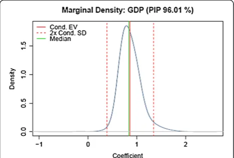
BMA allows the inclusion and exclusion of potential influences by means of a Markov Chain Monte Carlo (MCMC) samplerminvestigating the whole model space, i.e. the set of all possible variable combinations that can be employed to represent the dependent variable. In applying the BMA method, the uncertainty assessor firstly gathers any data that might be - even only in an indirect sense - be a relevant influence on the dependent variable. Let these candidate explanatory variables be k. The model space from which to choose the appropriate linear regression model is then 2k. Any variable could be included or excluded, reliant on the explanatory value for the dependent variable. This explanatory value is assessed as posterior inclusion probability (PIP) for individual explanatory variables, and the individual models (containing specific explanatory variables) are ranked according to their PMP. Hence, the explanatory power of each variable and of different competing linear regression models can be assessed. As the name indicates, these results of BMA are probabilities. The prior probabilities concern the assessors’ prior belief about how many explanatory variables are relevant. BMA then provides 1) the best linear regression model in terms of highest PMP and 2) the individual relevance of influences in terms of coefficient probability estimates and posterior inclusion probability PIP. In Figure 5, an exemplary coefficient estimate for an explanatory variable (GDP) of the natural gas price is illustrated.
On the abscissa, the coefficient value for the variable in the linear regression model is quantified. The ordinate represents the probability density for the coefficient
value (i.e. the rate of change of the conditional mean of the natural gas price conditional on the change of GDP). The double conditional standard deviation (2× cond. SD) is indicated in the red dotted line. An equivalent chart can be produced for every explanatory variable of the compet-ing models. The PIP of this variable is 96.1% what reflects that if the variable was contained in a model, competing models were less successful in explaining the data. In other words, the PIP is the sum of PMPs for all models wherein a covariate was included. The shape of the probability density and the low range of double standard deviation (approx. 0.4 to 1.4) indicate that variation from the conditional expected value (cond. EV) is rather low.
In practice the approach can be detailed in several steps. In step one, relevant input variables, or all input variables - depending on the size of the energy model under scrutiny - are identified, e.g. GDPo within the energy models’system boundary. In the next step, stat-istical data of economic, ecological, social or from other disciplines is gathered that is suspected to influence the input variable (e.g. statistical data concerning, industrial production, import and export, taxes and subventions, birth and death rates, education, etc.), including statistical data of the input variable. This input variable (GDP) in the uncertainty assessment becomes the dependent vari-able on these influences. Note that, in contrast to other methods, there are hardly practical limitations to the amount of influences that can be considered, for BMA by means of a MCMC sampler investigates the model space and ranks explanatory variables (influences) according to their PIP. The next step is the definition of the form of mathematical representation, e.g. a multivariate linear regressionp. As many potential explanatory variables are defined, the question is what variables should be included in the model. BMA estimates models for all possible combinations of explanatory variables and constructs a weighted average over all of them. Then, the choice of
a suitable prior distribution is defined, e.g. Zellner’s g-prior [61,62]. If the integrated likelihood is constant over all models, the PMP is proportional to the mar-ginal likelihood of a specific candidate model, i.e. the probability of the data given that model times a prior probability. The prior probability reflects how probable the expert thinks the model is before looking at the data [63]. The thence generated models with highest PMPs can be evaluated, and a model that best repre-sents the dependent variable (e.g. GDP) can be chosen. Finally, the uncertainty estimation for the input variable is derived from the PMP of the model chosen.
An additional feature that is not the focus of this text is the possibility of generating predictive distribution functions from the chosen model that consistently with past evidence and expert judgement represent the dependent variable for given assumptions of explanatory variables. This could foster consistency in the choice of key assumptions.
The interpretation of BMA results as uncertainty can be straight forward if uncertainty is suitable defined. To that end, a definition that is based on probability is introduced.
Definition: Uncertainty equals the probability that statement S might not be true.
Given, by means of BMA, a PMP is calculated for an uncertainty model (e.g. a PMP of 13%qfor a model that represents the natural gas price), uncertainty - by defin-ition - would be at least 87% for the dependent variable. This would mean that the input variable ‘natural gas price’ to an energy model holds an uncertainty of at least 87%, even if all relevant explanatory variables are considered. Hence, the results of a model including an assumption about the natural gas price cannot be less uncertain than 87%.
In other words, the PMP reflects the probability that the input variable thusly described matches data. For a model with a PMP of 13%, the associated uncertainty would be at least 87%. A clarifying statement of the following form could accompany model results.
“In consideration of expert judgement, statistical data of influence X1, influence X2, influence X3,…, of the last
25 years, the uncertainty that the input variable can be described as such is at least 87%.”
For every influence X1, X2,…, the PIP indicates the
explanatory contribution of the influence and 1-PIP indicates the uncertainty that the influence contributes to explaining the dependent variable of a given model (typically the one with the highest PMP). In the example, the uncertainty that GDP explains the natural gas price (together with the other explanatory variables) of the chosen model is 3.99% (1−0.9601 = 0.0399). Such an assessment clearly satisfies requirement 1 as uncertainty expressed as probability density is a clear indication how reliable the findings are.
The third virtue of expert knowledge, inclusion and exclusion of relevant factors, could be achieved by this standardised method, hereby satisfying requirement 2 (applicable independent of assessor’s expertise).
The approach would limit many intuitive over- or under-estimations of impact of influences on variables that figure as input variables in energy models. It is think-able that different experts evaluate individual influences as more/less relevant for the assumption of an input variable (e.g. a natural gas price assumption) thereby generating ambiguousness and dissent. A standardised method, rely-ing on statistical data, i.e. knowledge with little associated uncertainty in and by itself, could yield significant im-provement in uncertainty assessment for energy models. However, as expert knowledge is an important part of assessment methods, it is possible to take this by prior probability specification into account.
A key quality of the BMA method for input variables is that model uncertainty of the linear regression model itself, and thus, the assessment method’s uncertainty is quantified in probabilistic terms. This is a distinct advan-tage of the method as opposed to purely statistical or qualitative methods. Other methods that are applied in uncertainty analysis, for example, standard statistical ana-lysis or purely qualitative methods ignore that source of uncertainty. A standard regression analysis is conditional on the assumed statistical model, and the analyst may be uncertain whether it is the best representation. If an expert Delphi [64,65] is carried out opinions are rarely scrutinised for their correctness or compliance with statis-tical evidence. However, if an expert is asked, how prob-able she thinks her evaluation is, a prior distribution could be constructed.
Another requirement previously defined is the applicability to different energy models (comparability of results), requirement 3. As indicated by Figure 4, the assessment method is concerned with input data to energy models and is hence independent of the mathematical model that consequently processes the input. The uncertainty assessment method would be applicable for different kinds of models common in energy economics, LP’s, MCP’s, CGE’s, stochastic models or even qualitative models that use input variables.
Requirement 4 (inclusion of qualitative and quantitative aspects) to assure a complete representation can be achieved through prior probabilities and statistical data. The resulting posterior probabilities and the probabilistic interpretation of uncertainty are straightforward to com-municate, as demanded in requirement 5 (intuitively understandable and straightforward to communicate).
choice. This lies, as previously discussed, in the very na-ture of expert judgement. A sensitivity analysis to evaluate such ambiguousness could both, increase understanding of the BMA method within this context, and indicate to what extent expert elicitation has to be put in perspective to statistical data.
Results and discussion
Results of applying BMA to energy model input variables are PMPs of competing models for input variables of an energy model. The PMPs of the input variables can then be used to define quantitatively the associated uncertainty of the specific input variable. The method respects previ-ously defined requirements. The result is an uncertainty assessment of the form: applied input variableXhas an as-sociated uncertainty of at least Y%. Results of the model are thus associated with an uncertainty of at least Y%. Note, that such a result demands acceptance of the premise that model results cannot be less uncertain than model input.
Existing uncertainty assessments for energy models pro-vide evaluations of energy models or energy scenarios. However, the approaches discussed in this text lack some qualities in the context of energy modelling that BMA for input variable uncertainty estimation could provide.
The method described by Walker et al. is rather a classi-fication of uncertainty than an assessment that explicitly states uncertainty of results (requirement 1). On the other hand, methods that are applied in classical uncertainty quantificationrsuch as statistical analysis, stochastic mod-elling or error propagation computation, although being explicit, treat uncertainties in a mechanistic way that does not respect the various social and political aspects (requirement 4). Methods that mainly rely on expert elicitation, such as the NUSAP method might lack repro-ducibility of results and objectiveness (requirements 2 and 6). BMA could potentially combine the desired qualities. Intuitively understandable (requirement 5) uncertainty assessments that can be produced for different energy models (requirement 3) only dependent on the respective input variables the model demands could provide relevant insight in uncertainties that are associated with model input. As potential consequence of applying BMA for input variable uncertainty, transparency regarding model results with respect to the reliability of such findings could be evaluated and communicated. Moreover, input vari-ables could be classified according to their adherent uncertainty if the method is applied. And finally, but left for further research, the possibility of generating predictive densities by means of BMA could lead to consistent input variable values that respect influences across system boundaries of a specific model.
All uncertainty assessment methods have advantages and disadvantages. In spite of the successful fulfilment of
previously defined requirements, the BMA approach for input variables has deficits that need to be discussed.
A rather practical issue stems from the fact that the approach is parametric. This means that in practice, many different input variables need to be assessed if large and complex models are analysed and a significant amount of data collection and preparation seems neces-sary. One way, which proved successful in the NUSAP method, for reduction of assessment variables is a classi-fication of input variables and a consequent sensitivity analysis to discern highly relevant input variables [25]. Such a procedure could be suitable for the BMA approach as well.
Another issue might arise if input variables yield indi-vidual uncertainties of different orders of magnitude. The question then arises whether the least certain defines the uncertainty or if model dependent interpretation of indi-vidual uncertainties (of indiindi-vidual input variables) would be meaningful. It is not straightforward to see where in the mathematical core of energy models input variables are processed, and hence, tracing back results to individ-ual inputs could be difficult. A form of meta-analysis, as proposed by [66,67] could possibly give relevant insight regarding the uncertainty significance of individual input variables across studies of different model applications, as done for studies in medicine (psychotherapy) [68].
And finally, an issue could arise if an energy model incorporates aspects or effects that are relatively ‘new’, e.g. unconventional gas in Europe. Due to data scarcity and lacking maturity of available processes, a Bayesian approach to assess such input data would be difficult. The same problem of data scarcity can occur if scenario assumptions are not explicit, e.g. social, or psychological assumptions. If dataare available for such assumptions, their bearing on an input variable to an energy model can be incorporated by the BMA method and hence could increase transparency in that aspect. If data are not available, it must be communicated that the aspect is not part of the uncertainty assessment.
Conclusions
BMA for uncertainty quantification of input variables could potentially satisfy the requirements that a versatile applicable and standardised method for uncertainty assessment in energy economic modelling demands. Given the described advantages and disadvantages, it is at least worth discussion whether such an approach could improve the assessment itself and consequently could put the inferences and policy recommendations based on model results in perspective. This in turn should enable stakeholders and decision makers to include reported uncertainties in their decision making processes and increase trust in scientific findings. Trust in scientific findings is not solely generated by unerring model results but also by acknowledgement and trans-parency of uncertainties respecting that reality is not strictly deterministic.
Further research should be undertaken concerning the critical remarks and potential solutions for the applica-tion of the method. To this end, firstly an applicaapplica-tion of the approach to different models should yield insight allowing for further improvement of the approach.
Endnotes
a
For further information on energy models as referred to in this text see [70-72], or [73] in Germany.
b
The green kite is spanned up by the minimum scores in each group for each pedigree criterion; the orange kite is spanned up by the maximum scores. The orange band between the green kite and the red area represents expert disagreement on the pedigree scores for that variable. In some cases, the picture was strongly influenced by a single deviating low score given by one of the six experts. In those cases, the light green kite shows what the green kite would look like if that outlier would have been omitted.
c
Given that the same experts evaluate many fields of model-associated uncertainties, it is thinkable that the ex-pertise in some areas is not as sound as one would expect.
d
e.g. Limited number of experts, limited knowledge of experts.
e
However, Smithson [74] has made a strong case that ‘in all tasks, precise-conflictive sources were viewed as less credible than ambiguous-consensual ones even when subjects expressed preference for the precise-conflictive alternative.’what suggests that the require-ment of inter-subjectivity has more relevance in terms of acceptance of the assessment.
f
This might trace back to a criticism of [35] on the interdependence of likelihood and confidence:‘When an event is said to be extremely likely (or extremely unlikely) it is implicit that we have high confidence’.
g
As defined by [35], uncertainty that results from myr-iad factors both scientific and social and consequently is difficult to accurately define and quantify.
h
Qualification of the degree of agreement: summary terms: low, medium or high [29].
i
By that is meant that the uncertainty captured between 2 and 3 is not more/less than the uncertainty captured between 4 and 5, or for that matter 5 and 6.
j
For more information see for example [75-77].
k
e.g. Experts could be questioned what probability to a qualitative assessment like ‘surely no more/less than’ can be attributed. In that way, a subjective degree of belief can lead to a subjective prior distribution. See also [78,79].
l
Such as [80,81].
m
One could also use a Bayesian Markov chain Monte Carlo (BMCMC), as for example, Kim et al. have done to determine optimum tender prices [82].
n
This result stems from work not published yet, avail-able from the author. Abbreviations: GDP gross domestic product, PIP posterior inclusion probability, Cond. EV Conditional expected value, SD standard deviation. Note that, the shape of the probability distribution offers a further indication of the reliability of the conditional expected value.
o
Note that, input variables may vary considerably be-tween models. For example, a bottom up model as the TIMES linear program [2] does not enter economic performance directly in form of a GDP input variable. Instead, such macro-economic assumptions must be translated in sectorial demands, e.g. megakilogrammes of crude steel demand. This transformation is often done based solely on expert judgement for a given sector of an energy model. A BMA uncertainty assessment could improve transparency with regard to that process. An example of a demand forecast is industrial production is provided by [83].
p
Of course other models can be applied as well, for example, generalised linear models, proportional hazard models or logistic regressions.
q
A posterior model probability (PMP) of ca. 11% is a rather poor model representation of observed data. However, similar approaches in other contexts show that low PMPs are not unusual, e.g. infrastructure PMP 0.39 [84], econometric context PMP 0.3 [85], medical context PMP 0.17 in a dataset on primary biliary cir-rhosis [44] or [86]. For an explicit application to fore-casts, see [69]. For a BMA example in the context of hydrology, where the BMA method was coupled with a maximum likelihood estimation proposed by Taplin, see [87].
r
Mainly applied in engineering.
s