Open Access
Research article
The effect of tidal forcing on biogeochemical processes in intertidal
salt marsh sediments
Martial Taillefert*
1, Stephanie Neuhuber
1,2and Gwendolyn Bristow
1Address: 1School of Earth and Atmospheric Sciences, Georgia Institute of Technology, 311 Ferst Drive, Atlanta, GA 30332-0340, USA and 2Department of Geodynamics and Sedimentology, University of Vienna, Althanstrasse 14, 1090 Vienna, Austria
Email: Martial Taillefert* - [email protected]; Stephanie Neuhuber - [email protected]; Gwendolyn Bristow - [email protected]
* Corresponding author
Abstract
Background: Early diagenetic processes involved in natural organic matter (NOM) oxidation in marine sediments have been for the most part characterized after collecting sediment cores and extracting porewaters. These techniques have proven useful for deep-sea sediments where biogeochemical processes are limited to aerobic respiration, denitrification, and manganese reduction and span over several centimeters. In coastal marine sediments, however, the concentration of NOM is so high that the spatial resolution needed to characterize these processes cannot be achieved with conventional sampling techniques. In addition, coastal sediments are influenced by tidal forcing that likely affects the processes involved in carbon oxidation.
Results: In this study, we used in situ voltammetry to determine the role of tidal forcing on early diagenetic processes in intertidal salt marsh sediments. We compare ex situ measurements collected seasonally, in situ profiling measurements, and in situ time series collected at several depths in the sediment during tidal cycles at two distinct stations, a small perennial creek and a mud flat. Our results indicate that the tides coupled to the salt marsh topography drastically influence the distribution of redox geochemical species and may be responsible for local differences noted year-round in the same sediments. Monitoring wells deployed to observe the effects of the tides on the vertical component of porewater transport reveal that creek sediments, because of their confinements, are exposed to much higher hydrostatic pressure gradients than mud flats.
Conclusion: Our study indicates that iron reduction can be sustained in intertidal creek sediments by a combination of physical forcing and chemical oxidation, while intertidal mud flat sediments are mainly subject to sulfate reduction. These processes likely allow microbial iron reduction to be an important terminal electron accepting process in intertidal coastal sediments.
Background
Salt marshes are coastal regions of high primary produc-tivity [1,2] and receive substantial input of terrestrial organic matter [3]. Simultaneously, high rates of natural organic matter oxidation are recorded in salt marshes [4],
and evidence suggests that secondary production in these environments depends more on estuarine primary pro-duction than terrestrially-derived organic matter [5]. In fact, these ecosystems are very often either balanced between autotrophy and heterotrophy [5] or carbon lim-Published: 13 June 2007
Geochemical Transactions 2007, 8:6 doi:10.1186/1467-4866-8-6
Received: 21 February 2007 Accepted: 13 June 2007
This article is available from: http://www.geochemicaltransactions.com/content/8/1/6
© 2007 Taillefert et al; licensee BioMed Central Ltd.
ited [4,6,7]. Salt marshes have been proposed to be a net sink of CO2 from the atmosphere, though remineraliza-tion of carbon exported to continental margins may in fact be a source of CO2 to the atmosphere [8]. To predict the relationship between the different carbon reservoirs, it is necessary to understand the processes controlling organic carbon preservation in coastal marine sediments, including salt marshes. Unfortunately, the complex inter-action between physical, biological, and chemical proc-esses in salt marsh sediments limits our ability to quantify the biogeochemical cycling of elements in these systems.
Physical (sediment transport, tidal pumping, wave action, bioturbation), chemical (oxidation-reduction, precipita-tion-dissolution, adsorption), and microbial processes regulate the cycling of elements in intertidal sediments. Traditionally, the high complexity of salt marsh sediment biogeochemistry has been attributed to physical mixing by bioturbation. Macroorganisms mix the sediment [9] and irrigate their burrows with dissolved oxygen [10,11]. Irrigation may also occur through the roots of Spartina alterniflora [12]. Since bioturbation influences biogeo-chemical processes, it is often considered an important forcing parameter in field studies. Bioturbation has been suggested to be responsible for the oxidation of surficial sediments [e.g., [9,13,14]], the higher rates of iron reduc-tion measured compared to sulfate reducreduc-tion [15], and the high heterogeneity of microbial populations [16].
Interestingly, biogeochemists have paid little attention to the role of tidal forcing in intertidal salt marsh sediments. These environments are characterized by complex subsur-face hydrologies regulated by the marsh topography and sedimentology, influence of groundwater discharge as well as tidal pressure and wave action [17-21]. In some marshes, the subsurface flow is predominantly horizontal while, in others, water moves vertically [22]. Vertical flow can be generated at rising tide by overlying water infiltra-tions or water discharge to the overlying waters [22,23]. Infiltrations may either take place when water fills empty pore spaces above the water table [24], when cold overly-ing waters mix with porewaters warmed at low tide duroverly-ing the day [25], or as a result of the interaction of overlying water flow and rippled beds or mounds [21]. Simultane-ously, vertical flow can also be generated at ebb tide if the hydrostatic pressure is increased at depth and forces the porewaters to the surface [24]. Vertical flow is usually favored in marshes with flat topography, in coarse-grained sediments, in rippled sediments, or in confined zones such as creeks surrounded by banks. In turn, high lateral flow may occur if preexisting sediment structures, such as shallow confined permeable layers [22] or mounds [23], force a portion of the tidal flow in the hor-izontal direction.
The complexity of hydrological processes in intertidal salt marsh sediments coupled with the generally significant bioturbation, the high content of organic matter, and large sediment heterogeneities probably affect biogeo-chemical processes over a variety of spatial and temporal scales. As a result, new strategies to investigate these proc-esses with a high spatial and temporal resolution have to be adopted. Voltammetric techniques are attractive to measure redox chemical species involved in diagenetic processes in situ because several analytes can be detected simultaneously, their detection limits are reasonably low, and high spatial and temporal resolutions can be achieved [26].
Brendel and Luther [27] developed a mercury-gold amal-gam (Au/Hg) voltammetric microelectrode for the quan-tification of dissolved O2(aq), Fe2+, Mn2+, and ΣH
2S as well
as the qualitative determination of FeS(aq) [28] and solu-ble organic-Fe(III) complexes [30] that may be pervasive in marine sediments. Depth profiling in sediments have mostly included single electrode measurements after col-lecting sediment cores [e.g., [12,27,29,31-33]]. In turn, several microelectrodes have been used simultaneously to determine the three-dimensional distribution of redox chemical species in sediment cores [13] and in situ in salt marsh sediments [34], continental margin sediments [35,36], and deep-sea hydrothermal vents [37]. These techniques have yet to be used to study the dynamic bio-geochemical cycling of redox chemical species in inter-tidal salt marsh sediments.
The objectives of this project were to investigate the role of tidal forcing on the biogeochemistry of intertidal salt marsh sediments. To show that traditional sediment sam-pling and ex situ analysis with high spatial resolution can provide information relevant to seasonal variations in intertidal sediments, we present four years of ex situ pore-water measurements with Au/Hg voltammetric microelec-trodes at two different sites in the same salt marsh. To demonstrate that tides may have an important effect on the biogeochemical signatures of porewaters and the solid phase over short time and spatial scales, we compare tra-ditional sampling techniques and ex situ voltammetric analyses over a tidal cycle with in situ depth profiling with Au/Hg voltammetric microelectrodes. Finally, to deter-mine the effect of tidal forcing on the biogeochemistry of salt marsh sediments we correlate in situ measurements obtained with several microelectrodes positioned at dif-ferent depths and porewater movements measured during several tidal cycles at the two different sites.
Sampling Site
located off the Georgia coast, approximately 5 miles south of Savannah (Figure 1). The salt marshes on the East Coast of North America cover an area of 589,429 ha [38] and developed in an intertidal region in the back of a barrier-island system. In general, the sedimentological composi-tion of salt marshes in the Georgia bight are characterized by muddy sediments. These deposits are part of the Pleis-tocene/Holocene Satilla Formation [39] and of the Holocene Silver-Bluff terrace [40]. This terrace marks the last sea level highstand of about 1.8 m above present day sea level.
SERF includes a 213 m long boardwalk which provides direct access to the Skidaway Island salt marsh. This boardwalk spans a range of environments, from an inland salt marsh meadow to a tidal creek. This area is isolated from the nearby river (Figure 1) and not exposed to wave actions created by boats or winds. All the measurements reported were performed in the low marsh, where water levels vary between 1.5 m for neap tides and 2 m for spring tides (USGS web site). More than fifty small sedi-ment cores were collected along the boardwalk and ana-lyzed for porewater and solid phase composition over a period of four years at SERF (Table 1). This study reports
analyses performed at two sites along the boardwalk only (Figure 1): The mud flat site (MF), located 122 m from the island; and the creek bank site (CB), located 168 m from the island. The MF site is centered in an approximately 400 m2 unvegetated area of the marsh. In 2005, short Spartina began to grow in the area of study, but its density is not as high as other areas of the marsh. The sediment at MF is flat and exposed to the atmosphere for about 6 hours during each tidal cycle. Several small perennial creeks supply water to the site at rising tide. As a result, the water reaches the site as a front. The CB site is located in a perennial creek adjacent to the main creek at the end of the boardwalk (Figure 1). The creek is about 2.5 m wide at high tide and 1.5 m deep. Its banks are unvegetated but surrounded by a high Spartina field. The bottom of the creek is flat and about 1–2 m wide. Its sediment bed, where all the measurements were performed, is exposed to the atmosphere for about 3 hours per tidal cycle. The water is supplied to the site at rising tide through the main adjacent creek. Grain size analyses showed that 50% in weight of both sediments are well sorted fine grained sed-iments (< 75 µm in size). In average, the sizes of 10% of the sediment (d10) and 20% of the sediment (d20) are
approximately 3 and 17 µm, which correspond to silty clays [41].
Methods
At each of the MF and CB sites, four monitoring wells were installed in a row, 30 cm apart from each other, to moni-tor porewater pressures as a function of depth and time in the sediment during tidal cycles. Each well was made of 3 m long PVC pipe of 3.8 cm diameter sealed at the bottom and contained a single 0.15 mm slotted screen approxi-mately 5 cm long positioned at different interval from the bottom of the wells (i.e., 120, 105, 90, and 60 cm). At each site, the four wells were gently inserted in the sedi-ments such that the screens were located at the sediment-water interface (SWI), 15, 30, and 60 cm below the SWI. The wells were not submerged at high tide and were cov-ered with lose fit caps to prevent potential interferences from precipitations and avoid overpressurization. Water levels were determined in the monitoring wells by pres-sure transducers (Leveloggers, Solinst) corrected for meas-ured atmospheric pressure (Barologger, Solinst). Unless indicated, they were not corrected for the difference in screen height between the wells, such that differences of 15, 30, and 60 cm remain between the water levels of the well positioned at the SWI relative to the others at all time.
Ex situ geochemical measurements were obtained in sedi-ment cores collected directly from the boardwalk with a sediment corer made of a 50 cm long and 7.5 cm diameter polyacrylic liner closed with a polyacrylic cap. The cap contained an exhaust that was opened and sealed remotely when the corer was, respectively, inserted in and
Geographic location of Skidaway Island, the Salt marsh Eco-system Research Field station (SERF), and sampling sites along the boardwalk across the salt marsh
Figure 1
Geographic location of Skidaway Island, the Salt marsh Eco-system Research Field station (SERF), and sampling sites along the boardwalk across the salt marsh. The mud flat site (MF) is located 122 m from the island in the unvegetated part of the salt marsh. The creek bank site (CB) is located 168 m from the island in a perennial channel off the main creek. Four monitoring wells (mw), positioned approximately 30 cm apart, were inserted at each site to monitor fluid advection. Arrows indicate direction of the surface water flow at ebb tide.
Skidaway Institute of Oceanography
SKIDAWAY ISLAND SAVANNAH
SERF
GA SC
FL
Skidaway Island
CB MF
Low Spartina High Spartina
Unvegetated
Skidaway Island
removed from the sediment. A long pole was connected to the sediment corer to collect submerged sediment from the water surface. The sediment was removed by gently pulling the corer while maintaining the cap sealed. Coring at each site was performed within a 1 to 2 m radius when sampling periods were too close to each other to limit arti-facts due to the removal of sediment. Sediment cores were carefully transported to the laboratory located less than a kilometer away. When possible, sediments were collected with a large volume of overlying water to avoid disturbing the SWI. At low tide, when the volume of overlying water was small, capping the sediment with a rubber plug helped in preserving the integrity of the SWI during the short trip to the laboratory.
Ex situ and in situ voltammetric measurements were obtained with mercury-plated gold (Hg/Au) microelec-trodes. A three electrode system, consisting of an Ag/AgCl reference electrode, the Hg/Au microelectrode as working electrode, and a Pt counter electrode, was used for these measurements. Ex situ depth profile measurements were performed within 30 minutes after collection with a com-puter-operated DLK-100 potentiostat and a portable micromanipulator that can be piloted remotely by the computer (Analytical Instrument Systems, Inc.). For these measurements, a working electrode was positioned in an electrode holder and the reference and counter electrodes were attached to the side of the core liner such that they remained in the overlying waters [13]. The electrode was positioned above the SWI, and voltammograms were recorded as a function of depth in at least triplicates. In situ measurements were conducted with a 50 by 100 cm
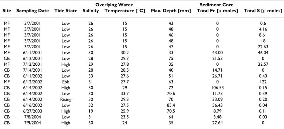
rectangle benthic lander specifically designed for deploy-ments from the board walk. The four-footed lander was fitted with a voltammetric system to analyze the porewa-ter composition as a function of depth and time over tidal cycles. The In Situ Electrochemical Analyzer (ISEA, Analyt-ical Instrument Systems, Inc.) consisted of a potentiostat encased in a waterproof pressure housing and an under-water micromanipulator (Analytical Instrument Systems, Inc.) operated by the potentiostat. With this system, up to eight voltammetric electrodes can be deployed in situ with a holder that carries all the electrodes within a 3 cm diam-eter circle. In situ depth profiles were first collected with a single working electrode that was lowered with vertical increments varying between 1 and 2 mm. For these meas-urements the reference and counter electrodes were posi-tioned in a separate holder against one of the feet of the lander such that they were always located in the overlying water. The position of the SWI was estimated from the sharp decrease observed in the voltammetric noise upon reaching the sediment surface. In a second series of in situ measurements, an array of up to five electrodes were deployed at fixed depths in the sediment to collect time series data during tidal cycles. For each of the time series deployments, the tip of the uppermost working electrode was positioned at a known height from the tips of the ref-erence and counter electrodes on the same electrode holder, and the tips of the remaining electrodes were posi-tioned at fixed heights from each other. The micromanip-ulator was then lowered to position the reference and counter electrodes at the SWI. The lander was always deployed at low tide, when the sediment was exposed to the atmosphere, such that the reference and counter elec-Table 1: Sites description, overlying water conditions, and properties of the sediment cores collected at SERF between 2001 and 2004.
Overlying Water Sediment Core
Site Sampling Date Tide State Salinity Temperature [°C] Max. Depth [mm] Total Fe [µ moles] Total S [µ moles]
MF 3/7/2001 Low 26 15 43 0 0.6
MF 3/7/2001 Low 26 15 48 0 4.16
MF 3/7/2001 Low 26 15 46 0 8.61
MF 3/7/2001 Low 26 15 48 0 18
MF 3/7/2001 Low 26 15 47 0 22.63
MF 6/11/2001 Low 30 30.2 33 43.00 46.04
CB 6/12/2001 Low 28 29.7 75 21.53 0
MF 7/13/2001 High 29 27.8 35 0 32.57
CB 7/14/2001 Low 28 28.5 40 14.71 0
CB 6/11/2002 Low 33 27.6 51 26.71 0.43
MF 6/12/2002 Ebb 31 27.7 63 0 122
CB 6/14/2002 High 30 29 72 106.53 0.15
CB 6/14/2002 Low 30 33.7 70.6 11.73 0.39
CB 6/14/2002 Rising 30 29.3 70 33.09 0.20
CB 6/16/2002 Low 32 27.5 85.4 56.43 0.04
CB 6/27/2003 High 19 25.9 70.5 8.79 0.11
CB 7/8/2004 Low 31 23.5 64 3.48 0.03
trodes could be positioned as close as possible to the SWI using a coarse micromanipulator displacement setting. The electrode system was then lowered with a fine millim-eter resolution, and voltammetric scans were acquired after each spatial increment until the electrodes made con-tact with the SWI. The SWI was inferred to be the location at low tide where the counter and reference electrodes were in electrical contact with the uppermost working electrode.
Au/Hg working microelectrodes were manufactured as previously described [30-32] and calibrated by the pilot ion method [27]. Working microelectrodes were fabri-cated from 4 mm diameter hollow glass pulled at one end under high temperature to form a tip of about 5 cm length and 1 mm diameter. A 100 µm gold wire was sealed into the glass tip with an Epoxy resin (West Marine) and con-tacted to a copper wire with Ag solder. Using this tech-nique, the electrodes were rigid and not influenced by water flow during tidal cycles. The electrode tip was sanded to a disk and then polished successively with 15, 6, 1, and 0.25 µm diamond pastes (Buehler). The gold disk was plated in a 0.1 M Hg(NO3)2 solution for 4
min-utes. The mercury film was then conditioned at -9 V for 90 seconds to form a better amalgam between the gold and the mercury. Linear sweep voltammetry (LSV) was exclu-sively used to measure dissolved oxygen (MDL ~4 µM), while cathodic square wave voltammetry (CSWV) was used to quantify Mn2+ (MDL ~15 µM), Fe2+ (MDL ~25
µM), and ΣH2S (= H2S + HS- + S2- + S
x2- + S(0), MDL ~0.2
µM) and detect FeS(aq) [28] and soluble organic complexes
of Fe(III) [30]. For these measurements, the potential was scanned from -0.1 V to -1.8 V after a conditioning period of 10 s at -0.1 V to clean the electrode between measure-ments. When soluble organic Fe(III) complexes or dis-solved sulfide were present, a conditioning step was also applied at -0.9 V for 10 s to remove these species from the electrode surface before the next measurement. When the concentration of dissolved sulfide was high, anodic square wave voltammetry (ASWV) was preferred to avoid formation of HgS double films [42]. Scan rates of 200 mV/ s were typically applied for all measurements. The chemi-cal composition of soluble organic-Fe(III) complexes and FeS(aq) are still unknown and cannot be quantified using
external calibrations. These species are therefore reported in voltammetric current intensities. Voltammetric data were processed with a home-built Matlab program [43] that integrates peaks (SWV) and derives waves (LSV). When voltammetric signals for Mn2+ and Fe2+ overlapped,
their currents were deconvoluted assuming voltammetric peaks display gaussian shapes [43]. Average and standard deviations reported represent a minimum of triplicate measurements.
After in situ voltammetric measurements, a sediment core was retrieved and sectioned in depth increments of about 5 mm to determine the chemical composition of the solid phase and measure porewater species not detectable by voltammetry (i.e. orthophosphate, nitrate, nitrite, total dissolved inorganic carbon). When ex situ voltammetric measurements were conducted, the same core was sec-tioned for porewater analyses, generally within a couple of hours after collection (the time it takes to complete ex-situ voltammetric measurements). All sediment process-ing was performed in a polypropylene glove bag (Aldrich) under N2 atmosphere to avoid oxidation of reduced
chemical species. Once sectioned, sediment layers were placed in 50 ml centrifuge tubes (Nalgene) and centri-fuged at 3000 rpm under N2 atmosphere for 5 to 10
min-utes to separate the porewaters from the solid phase. Porewaters were collected with acid-washed polypropyl-ene syringes (Norm-Ject, Henke Sass Wolf) and immedi-ately filtered in the glove bag through 0.2 µm polysulfone membrane Puradisc filters (Whatman). The filtrate was then split for immediate analysis (i.e., total dissolved inorganic carbon, orthophosphate) or frozen for further analysis, generally within 48 hours (i.e., nitrate, nitrite). The remaining sediment was sealed under N2 and frozen until analysis.
Orthophosphates (ΣPO43-) were measured in the
porewa-ters by spectrophotometry [44]. Amorphous iron oxides and total reactive iron were determined in the solid sedi-ment using the ascorbate and dithionite methods [45]. The ascorbate reagent extracts only amorphous forms of Fe3+ whereas the dithionite extractant dissolves
amor-phous iron oxides, acid volatile sulfide (AVS), and crystal-line iron oxides including magnetite, goethite, and to a lesser extent chlorite [45]. Triplicate wet sediment samples were leached with ascorbate at 25°C for approximately twenty four hours and with dithionite for approximately four hours in a 60°C water bath. Samples were then fil-tered, diluted, and analyzed by the ferrozine method [46]. Acid volatile sulfide (AVS) was extracted in triplicate sam-ples by cold distillation in 3 mol L-1 HCl under a N
2
atmosphere [47]. The volatile H2S gas was distilled for four hours and trapped in a 1 mol L-1 NaOH solution. An
aliquot of this solution was then analyzed voltammetri-cally for ΣH2S in 0.5 mol L-1 NaCl.
K = 0.36(d20)2.3 (1)
where d20 represents the average diameter of 20% of the particles in these sediments in mm, and K is the hydraulic conductivity in cm s-1.
Results
Generally, porewater profiles displayed contrasting chem-istries over the first 10 cm of sediment at the MF and CB sites, as shown in the typical examples of Figure 2. In MF sediments, porewater profiles generally contained lower concentrations of Mn2+ and Fe2+, but larger
concentra-tions of dissolved sulfide (Figure 2a). At the CB site, pore-waters contained low concentrations of dissolved sulfide, but larger concentrations of Mn2+ and Fe2+ (Figure 2a). In
addition, soluble organic-Fe(III) complexes were only detected in CB sediments, while FeS(aq) was generally observed below the onset of dissolved sulfide. Sometimes, FeS(aq) was detected close to the SWI, even in CB sedi-ments (e.g., Figure 2b). Total dissolved orthophosphate, while generally around the same concentration, also exhibited characteristic profiles at both sites. In MF sedi-ments, total dissolved orthophosphate reached the SWI, while in CB sediments, it was mostly present in the deep porewaters (Figure 2). The solid phase also displayed con-trasting depth profiles at both sites. In MF sediments, the concentrations of total extractable iron (dithionite Fe) and amorphous iron oxides (ascorbate Fe) were low with maxima at the SWI (Figure 2a). In CB sediments, the con-centrations of ascorbate and dithionite Fe were both high and homogeneously distributed (Figure 2b).
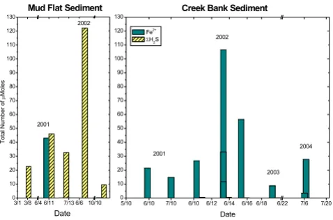
To compare geochemistries at both locations, depth-inte-grated mole contents of Fe2+ and ΣH
2S were determined in
each sediment core by summing, over the entire length of the sediment core, the number of moles measured in the volume of sediment delimited by the depth interval between measurements and the surface area of the sedi-ment core. These calculations assume that the concentra-tions measured electrochemically represent the average concentrations in each slice and that the porosity changes as a function of depth do not affect the concentrations sig-nificantly. The depth-integrated mole content of Fe2+ and
ΣH2S in the cores collected seasonally between 2001 and 2004 were clearly distinct at both sites (Table 1 and Figure 3). MF sediments contained high dissolved sulfide and low ferrous iron concentrations, while CB sediments were characterized by high concentrations of reduced iron and low concentrations of dissolved sulfide.
In an attempt to determine the role of tidal forcing on the biogeochemical processes in porewaters, a sediment core was collected from the CB site at three different times dur-ing the same tidal cycle (Figure 4). The first core, collected at high tide, displayed extremely high concentrations of both Mn2+ and Fe2+ right below the SWI and a dissolved
sulfide peak between 30 and 40 mm that reached rela-tively low concentrations (i.e. < 10 µM). Below 40 mm, Fe2+ was produced again, while Mn2+ had totally
disap-peared from the porewaters (Figure 4a). This core also generated low voltammetric currents for soluble organic-Fe(III) and FeS(aq). The second core, collected at low tide, displayed a similar profile but with much lower concen-trations in all the dissolved species mentioned above, except for the presence of a stronger voltammetric signal for soluble organic-Fe(III) between 20 and 40 mm (Figure 4b). At the next flooding tide, porewater profiles looked completely different, with dissolved Fe2+ that
progres-sively increased with depth and reached a maximum con-centration of 500 µM at 55 mm. Interestingly, the onset of dissolved sulfide was found at approximately the same location and range of concentrations as the other two cores (Figure 4c), while aqueous FeS showed a maximum just below the sediment water interface, was depleted at the depth of maximum dissolved sulfide, and increased below the zone of dissolved sulfide minimum. Soluble organic-Fe(III) was small near the SWI and increased below the sulfide minimum (Figure 4c). Total dissolved orthophosphate varied significantly during the tidal cycle. At high tide, it was close to detection limit (Figure 4a), at low tide it reached the SWI and displayed a typical tran-sient diffusive profile (Figure 4b), while at the following flooding tide, it exhibited the same transient diffusive pro-file but with an onset at 30 mm below the SWI (Figure 4c). Finally, the solid phase of the same sediment cores revealed curious heterogeneities in the creek. While its total reactive and amorphous iron oxides content were high and relatively constant with depth at high and flood-ing tide (Figure 4a and 4c), they were much lower in con-centration at low tide and displayed a maximum in the first 20 mm of sediment (Figure 4b). AVS measurements performed at low tide revealed low concentrations of FeS(s) in these surficial sediments. Since these sediment cores were collected within one meter of each other, these differences can only be attributed to lateral heterogenei-ties within the creek. The measurements clearly showed that the influence of tidal forcing on the biogeochemical processes in porewaters could not be considered using conventional sampling and analyses because sediment heterogeneities could not be discerned from temporal var-iations during tidal cycles.
In situ depth-profile measurements were conducted at both sites to capture the effect of tidal forcing on the geo-chemistry of porewaters. Each profile was completed within four hours after deployment during the fall season, when sulfate reduction is usually in decline. Surprisingly, the MF and CB sites revealed relatively similar geochemis-tries (Figure 5), with no significant soluble organic-Fe(III) (< 5 nA), Mn2+, and Fe2+ across the entire profiles,
Porewater O2(aq), Mn2+, Fe2+, ΣH2S, org-Fe(III)(aq), FeS(aq), and ΣPO43-, and ascorbate- and dithionite-extractable Fe as a function
of depth in sediment cores collected ex situ at: a) the mud flat site; and b) the creek bank site in the Skidaway Salt Marsh in June 2002
Figure 2
Porewater O2(aq), Mn2+, Fe2+, ΣH2S, org-Fe(III)(aq), FeS(aq), and ΣPO43-, and ascorbate- and dithionite-extractable Fe as a function
of depth in sediment cores collected ex situ at: a) the mud flat site; and b) the creek bank site in the Skidaway Salt Marsh in June 2002. All porewater chemical species, except ΣPO43-, were measured electrochemically in intact sediment cores. Mn2+
was below minimum detection limit (MDL) in the mud flat porewaters. Note the difference in the O2(aq) and Fe2+ concentration
scales between both sites.
100 90 80 70 60 50 40 30 20 10 0 -10
0 50 100 150 200 250
100 90 80 70 60 50 40 30 20 10 0 -10
0 200 400 600 800 1000 1200
0 20 40 60 80 100
0 250 500 750 1000 1250 1500 1750
100 90 80 70 60 50 40 30 20 10 0 -10
0 50 100 150 200 250 300 350
0 5 10 15 20 25 30
Ascorbate Fe, Dithionite Fe - [Pmole/g dry weight] O2(aq), Mn
2+
, Fe2+ - [PM]
D
ept
h
[m
m
]
6PO4
- [PM]
6H2S - [PM]
Fe(III)(aq) - [nA]
FeS(aq) - [nA]
70 60 50 40 30 20 10 0 -10
0 50 100 150 200 250
70 60 50 40 30 20 10 0 -10
0 50 100 150 200 250 300 350
0 250 500 750 1000 1250 1500 1750
70 60 50 40 30 20 10 0 -10
0 50 100 150 200 250 300 350
0 5 10 15 20 25 30 0 20 40 60 80 100
Ascorbate Fe, Dithionite Fe - [Pmole/g dry weight] O2(aq), Fe
2+
- [PM]
D
epth
[
m
m
]
6H2S - [PM]
Fe(III)(aq) - [nA]
FeS(aq) - [nA] 6PO4
- [PM] a)
for salt marsh sediments (< 30 µM), and small but detect-able levels of aqueous FeS. The accumulation of dissolved sulfide in the porewaters at both sites, on the other hand, displayed a rather distinct feature. In the MF sediment, it occurred sporadically at three distinct locations, 30, 75, and 105 mm below the SWI. In contrast in the CB sedi-ment, it formed a peak 15 mm below the SWI, just above the soluble organic-Fe(III) maximum.
Finally, several series of in situ measurements were obtained during tidal cycles using up to five electrodes positioned at different depths in the MF and CB sedi-ments. Figure 6 and Figure 7 display two examples of such measurements obtained within days of each other. These time series illustrated the extreme complexity of intertidal salt marsh sediments. They revealed rapid changes in con-centrations of Fe2+, dissolved sulfide, and current
intensi-ties of soluble organic-Fe(III) and FeS at each depth that seemed to correlate with water levels measured in the sed-iment with the monitoring wells and water levels above the sediment obtained from the NOAA buoy at Fort Pulaski. At the same time, they showed strong variations with depth, probably related to the heterogeneity of sedi-ments and the complex hydrologies at these sites. None-theless, important trends could be observed during tidal cycles. At low tide (before 15:30 and after 22:00), the MF sediment displayed high concentrations of reduced spe-cies (i.e., Fe2+ and ΣH
2S) at most of the depths surveyed
(Figure 6). At rising tide, ΣH2S seemed to initially be pro-duced at depth (Figure 6d–f), then consistently removed, while simultaneously produced at low concentrations in the overlying waters. Similarly, Fe2+ was initially produced
at the SWI and the overlying waters at rising tide (Figure 6b–c) but was removed completely when ΣH2S reached the overlying waters. Except at 3.5 cm, the removal of sulfide was not accompanied by the production of FeS(aq) complexes at depth. As these complexes are precursors in the precipitation of FeS(s) [28], precipitation of iron sulfide minerals did not appear responsible for the decrease in ΣH2S and Fe2+ concentrations at rising tide, at
least at the time of these measurements. These data instead suggest that porewater advection at rising tide pushed reduced species towards the SWI where Fe2+, and
possibly ΣH2S, were oxidized by dissolved oxygen. The
oxidation of Fe2+ was supported by the production of
sol-uble organic-Fe(III) complexes at the SWI and in the over-lying waters at rising tide (Figure 6b–c). At ebb tide, the concentrations of these species did either not change or decreased slightly as a function of time (Figure 6).
CB sediments behaved in a similar fashion. The concen-tration of reduced chemical species was generally high just below the SWI at low tide (Figure 7b–c) but changed at rising tide. First, Fe2+ was abruptly removed from the
surfi-cial porewaters at the onset of the tide change, before
ΣH2S appeared in the sediment layers. Interestingly, the removal of Fe2+ occurred at 1.7 cm first, then at 0.5 cm,
and was accompanied by the production of soluble organic-Fe(III) (Figure 7b–c), suggesting again that oxida-tion of Fe2+ took place in surficial sediments. Dissolved
sulfide was initially produced at depth at rising tide (Fig-ure 7b–d), then was slowly removed from the porewaters. The removal of ΣH2S was accompanied by the production
of FeS(aq) complexes close to the SWI (Figure 7b–c), sug-gesting that precipitation of FeS(s) could occur in CB sedi-ments. At ebb tide, the concentrations of Fe2+ and ΣH
2S as
well as current intensities of FeS(aq) and soluble organic-Fe(III) complexes did not change significantly (Figure 7b– e).
Similar in situ measurements were conducted over three years and at different seasons at the same sites. To com-pare the behavior of the different sites over tidal cycles, the average Fe2+ and ΣH
2S concentrations measured as a
func-tion of time at each depth and both sites was represented with the temporal deviation from their average concentra-tions as a function of depth in the sediment (Figure 8). This comparison confirmed the high temporal variations linked to tidal changes and revealed two main differences between MF and CB sediments. First, MF sediments dis-played higher concentrations of dissolved sulfide com-pared to the CB site, which could produce relatively high concentrations of Fe2+ (Figure 8). Second, the
concentra-tion of dissolved sulfides increased regularly with depth in MF sediments, while concentrations were much more var-iable with depth in CB sediments.
Depth-integrated Fe2+ and ΣH
2S mole content of the
pore-waters at the creek bank and mud flat sites over the last four years
Figure 3
Depth-integrated Fe2+ and ΣH
2S mole content of the
pore-waters at the creek bank and mud flat sites over the last four years. The number of moles was calculated assuming the porewater homogenous over the volume defined by the sed-iment core diameter and the vertical distance between meas-urements.
3/1 3/8 6/4 6/11 0 10 20 30 40 50 60 70 80 90 100 110 120 130
2002
2001
To
tal
N
u
m
ber
of
P
Mo
le
s
Date
5/10 6/10 7/10 0
10 20 30 40 50 60 70 80 90 100 110 120 130
Fe2+ 6H2S
6/10 6/12 6/14 6/16 Date
6/18 6/22 7/6 7/20 Mud Flat Sediment Creek Bank Sediment
6/6 10/10
2004
2003 2002
2001
Porewater O2(aq), Mn2+, Fe2+, ΣH
2S, org-Fe(III)(aq), FeS(aq), and ΣPO43-, and ascorbate- and dithionite-extractable Fe as a function
of depth in sediment cores collected ex situ at the creek bank site in the Skidaway Salt marsh at: a) High tide; b) Low tide; and c) Rising tide over a 24 hour period in June 2002
Figure 4
Porewater O2(aq), Mn2+, Fe2+, ΣH
2S, org-Fe(III)(aq), FeS(aq), and ΣPO43-, and ascorbate- and dithionite-extractable Fe as a function
of depth in sediment cores collected ex situ at the creek bank site in the Skidaway Salt marsh at: a) High tide; b) Low tide; and c) Rising tide over a 24 hour period in June 2002. Acid volatile sulfide (AVS) was quantified in the low tide sediment core only.
80 70 60 50 40 30 20 10 0 -10
0 200 400 600 800
0 20 40 60 80 0 2 4 6 8 10
80 70 60 50 40 30 20 10 0 -10
0 50 100 150 200
80 70 60 50 40 30 20 10 0 -10
0 500 1000 1500 2000
0 2 4 6 8 10 12 14
Ascorbate Fe, Dithionite Fe - [Pmole/g dry weight]
6PO
4
- [PM] FeS(aq) - [nA]
FeIII (aq) - [nA]
O2(aq), Fe 2+
- [PM]
De
pt
h -
[m
m
]
6H
2S - [PM]
80 70 60 50 40 30 20 10 0 -10
0 20 40 60 80 100
0 20 40 60 80 80
70 60 50 40 30 20 10 0 -10
0 50 100 150 200 250
80 70 60 50 40 30 20 10 0 -10
0 500 1000 1500 2000
0 2 4 6 8 10 12 14 0 2 4 6 8 10
Ascorbate Fe, Dithionite Fe, AVS - [Pmole/g dry weight]
6PO4
- [PM] FeIII
(aq) - [nA] O2(aq) Mn
2+ , Fe2+
- [PM]
D
epth -
[m
m
]
6H2S - [PM] FeS(aq) - [nA]
80 70 60 50 40 30 20 10 0 -10
0 50 100 150 200 250 300 350
0 20 40 60 80 0 2 4 6 8 10
80 70 60 50 40 30 20 10 0 -10
0 50 100 150 200 250
80 70 60 50 40 30 20 10 0 -10
0 500 1000 1500 2000
0 2 4 6 8 10 12 14
Ascorbate Fe, Dithionite Fe - [Pmole/g dry weight]
6PO 4
3- - [PM] FeS
(aq) - [nA] FeIII
(aq) - [nA] O2(aq), Mn
2+ , Fe2+
- [PM]
D
e
pth
[m
m
]
6H2S - [PM]
a)
b)
To correlate the geochemical changes with the movement of porewaters during tidal cycles, water levels were recorded in the monitoring wells adjacent to each site over more than three years, from June 2003 to August 2006. The change in water levels in the wells during tidal cycles was due to the variation in hydrostatic pressure in the sed-iment over time and reflected the movement of water in the sediment pores. MF water levels, monitored immedi-ately after the wells were installed, indicated that the SWI and 15 cm wells reached equilibration after approxi-mately 30 hours (Figure 9a). CB water levels were moni-tored only 52 hours after their installation and indicated
that the SWI and 15 cm wells were already at equilibrium (Figure 9b). In turn, water levels deeper than 30 cm in both the CB and MF sediments did not change signifi-cantly over tidal cycles, even after several months of equi-libration (not shown), suggesting that the permeability of these sediments was too low below that depth to be sus-ceptible to tidal variations. Interestingly, water levels obtained at 15 cm deep and near the SWI indicated that the hydrology at both sites was different. While the water levels in both wells at the CB site varied at relatively the same rate (Figure 9b), water levels at the SWI changed more rapidly than 15 cm below the SWI in MF sediments (Figure 9a). In addition, the relative change in water levels between low and high tide were smaller in MF than CB sediments. Finally, an approximate 15 minute phase lag was observed between the time the water rose in the SWI and 15 cm wells at the MF site (inset in Figure 9a); in
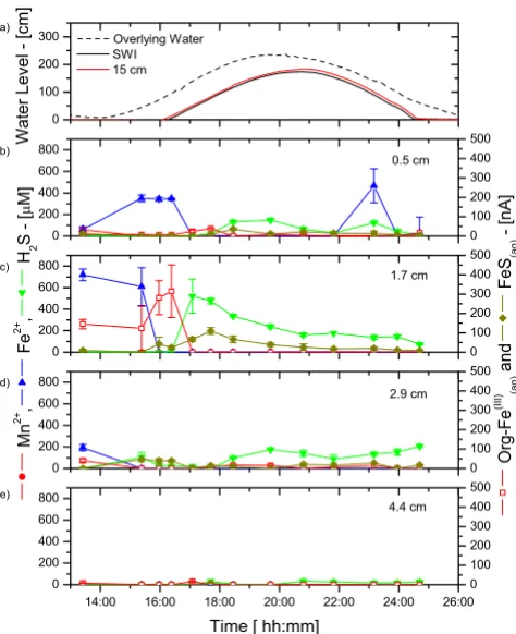
con-Water level changes (from low tide levels) and porewater Mn2+, Fe2+, ΣH
2S, org-Fe(III)(aq), and FeS(aq) measured in situ at
five fixed depths and as a function of time during a tidal cycle at the mud flat site in June 2003
Figure 6
Water level changes (from low tide levels) and porewater Mn2+, Fe2+, ΣH
2S, org-Fe(III)(aq), and FeS(aq) measured in situ at
five fixed depths and as a function of time during a tidal cycle at the mud flat site in June 2003. a) Well water levels meas-ured at the sediment-water interface (SWI) and 15 cm below the SWI, and tidal fluctuations obtained from the Fort Pulaski NOAA buoy; Concentrations (left) and current intensities (right) measured: b) in the overlying water; c) at the SWI; d) at 3.5 cm; e) at 7.0 cm; and f) at 10.5 cm. Dissolved oxygen was never detected in the porewaters.
0 100 200 300 0 500 1000 1500 0 50 100 150 0 500 1000 1500 0 50 100 150
12:00 14:00 16:00 18:00 20:00 22:00 24:00 26:00 0 500 1000 1500 0 50 100 150 0 500 1000 1500 0 50 100 150 0 500 1000 1500 0 50 100 150 SWI 15 cm W a te
r Level - [
c m] Overlying Water Org-Fe (II I) (aq) and Fe S(aq) - [nA]
Time - [hh:mm]
10.5 cm 7 cm 3.5 cm SWI
Fe
2+ and
H
2
S - [
P M] Overlying Water a) b) c) d) e) f)
Porewater Fe2+, ΣH
2S, org-Fe(III)(aq), and FeS(aq) measured in
situ as a function of depth with voltammetric Au/Hg microe-lectrodes at: a) the mud flat site starting at low tide; and b) the creek bank site starting at high tide in the Skidaway salt marsh in October 2002
Figure 5
Porewater Fe2+, ΣH
2S, org-Fe(III)(aq), and FeS(aq) measured in
situ as a function of depth with voltammetric Au/Hg microe-lectrodes at: a) the mud flat site starting at low tide; and b) the creek bank site starting at high tide in the Skidaway salt marsh in October 2002. Mn2+ was not detected in both
sedi-ments.
0 2 4 6 8 10 70 60 50 40 30 20 10 0 -10
0 2 4 6 8 10
70 60 50 40 30 20 10 0 -10
0 20 40 60 80 100
0 5 10 15 20 25 30 35 40 45 50
FeS(aq) - [nA]
FeIII
(aq) - [nA]
Mn2+
and Fe2+
- [PM]
De p th [ mm]
6H2S - [PM]
0 2 4 6 8 10 110 100 90 80 70 60 50 40 30 20 10 0 -10
0 2 4 6 8 10
110 100 90 80 70 60 50 40 30 20 10 0 -10
0 20 40 60 80 100
0 5 10 15 20 25 30 35 40 45 50
FeS(aq) - [nA]
FeIII
(aq) - [nA]
Mn2+
and Fe2+
- [PM]
D e pt h [ m m ]
6H2S - [PM]
a)
trast, a 15 minute lag was found between the 15 cm and SWI wells at the CB site (inset in Figure 9b). These data indicate that water percolated from the sediment surface to deeper depths at the MF site, while water advected from depth to the surface of the sediment at the CB site.
Discussion
Intertidal salt marsh sediments are extraordinarily com-plex environments that display extremely high temporal and spatial variabilities. Unfortunately, techniques able to measure multiple redox species simultaneously with a high temporal resolution and in several dimensions do not presently exist. The results of the present study were obtained with a combination of voltammetric microelec-trode and conventional porewater and solid phase analy-ses to gain better insights into the role of tidal forcing on the biogeochemistry of these sedimentary environments
near the sediment-water interface. The measurements, together with the numerous data obtained over the last four years at SERF [13,41,49-51] show that, in general, mud flat sediments are more reducing environments, with larger sulfide concentrations produced than in creek bank sediments, at least during the warm season (Table 1, Fig-ure 3). In contrast, creek bank sediments contain large concentrations of ferrous iron (Table 1, Figure 3) and sometimes reduced manganese (Figure 2, Figure 4).
Measurements of water levels (e.g., Figure 9) and temper-ature (not shown) in the monitoring wells of the MF and CB sites over more than three years indicate that the pore-waters deeper than 30 cm below the SWI at both sites are almost not influenced by tidal fluctuations. These data suggest that the permeability of these sediments generally decreases below that depth and limits water exchange dur-ing tidal cycles (Figure 9). Porosities measured in unvege-tated sediment cores confirm these findings: They vary between 86(+/-4)% at the surface to 70(+/-5)% around 50 cm and display a significant decrease below 20–30 cm depending on the sites (Clark Alexander, personal com-munication). As most geochemical investigations use sed-iment cores of less than 50 cm, conventional ex situ measurements in intertidal sediments should be carefully considered if the sediments are collected during flood or ebb tide and probably accompanied by a hydrological sur-vey. In contrast, well water measurements over the first 30 centimeters of sediment reveal significantly different hydrologies at the MF and CB sites. First, the MF wells
Average concentrations of Fe2+ and ΣH
2S measured in situ
during tidal cycles as a function of depth at: a) the mud flat site; and b) the creek bank site
Figure 8
Average concentrations of Fe2+ and ΣH
2S measured in situ
during tidal cycles as a function of depth at: a) the mud flat site; and b) the creek bank site. The standard deviations rep-resent temporal variations from the average concentration during tidal cycles. The number of tidal cycles during which concentrations were measured and the date of these meas-urements are provided above each data set.
0 2 4 6 8 0.0 0.5 1.0 1.5 2.0 2.5 8 9 10
0 2 4 6 8 0 1 2 3 4 5 6 7 8 9 10 Average Concentrat
ion - [
mM]
-5 0 5 10
1 Tidal Cycle January 2003
1 Tidal Cycle January 2003
8 Tidal Cycles June 2006 2 Tidal Cycles
July 2004
1 Tidal Cycle June 2003 5 Tidal Cycles
June 2006
1 Tidal Cycle June 2003
0 1 2 3 4 5
Fe2+
6H
2S(aq)
0 5 10 15
Depth - [cm]
0 5 10
Creek Bank Sediment Mud Flat Sediment
0 5 10
Depth - [cm]
Water levels changes (from low tide levels) and porewater Mn2+, Fe2+, ΣH
2S, org-Fe(III)(aq), and FeS(aq) measured in situ at
four fixed depths and as a function of time during a tidal cycle at the creek bank site in June 2003
Figure 7
Water levels changes (from low tide levels) and porewater Mn2+, Fe2+, ΣH
2S, org-Fe(III)(aq), and FeS(aq) measured in situ at
four fixed depths and as a function of time during a tidal cycle at the creek bank site in June 2003. a) Well water level changes (from low tide levels) measured at the sediment-water interface (SWI) and 15 cm below the SWI, and tidal fluctuations obtained from the Fort Pulaski NOAA buoy; Porewater concentration (left) and current intensities (right) at: b) 0.5 cm; c) 1.7 cm; d) 2.9 cm; and e) 4.4 cm. Dissolved oxygen was never detected in the porewaters.
0 100 200 300 0 200 400 600 800 0 100 200 300 400 500 0 200 400 600 800 0 100 200 300 400 500
14:00 16:00 18:00 20:00 22:00 24:00 26:00 0 200 400 600 800 0 100 200 300 400 500 0 200 400 600 800 0 100 200 300 400 500 SWI 15 cm Wa te r L e v e
l - [cm] Overlying Water
4.4 cm 2.9 cm Org-Fe (I II ) (aq) and FeS (a q ) - [nA]
Time [ hh:mm]
0.5 cm Mn 2+ , Fe 2+ , H 2
S - [
equilibrate at a slower rate than the CB wells (e.g., Figure 9), suggesting that hydrostatic pressure gradients in mud flat sediments are lower than in creek sediments. Second, the average exposure time of the sediment to the atmos-phere at low tide, obtained from five series of measure-ments over more than three years, is about twice as much longer at the MF site (366(+/-64) min) than the CB site (184(+/-74) min). Finally, the delay between the time at which water levels change in the SWI and 15 cm wells dur-ing risdur-ing tide at both sites indicates that porewaters advect in the vertical direction at both sites, though water seems to percolate from the surface in the mud flat while porewater is transported from the deeper depths to the sediment surface in creek sediments. Because of the close proximity of the four different wells at each site (less than 15 cm apart), water levels only provide the vertical com-ponent of the fluid advection, and we cannot exclude the
fact that porewater may overall move in the horizontal direction with a significant vertical contribution. Never-theless, the difference in hydrostatic pressure gradients at the CB and MF sites can be explained if hydraulic conduc-tivities are distinct. Interestingly, hydraulic conducconduc-tivities estimated from the particle sizes and Eq. 1 vary approxi-mately between 6 10-7 and 6 10-5 cm s-1 with depth in the
sediment at both sites (not shown). Given the level of incertitude of these measurements, these variations are not significant between sites. They compare well with con-ductivities of other fine-grained salt marsh sediments [52], but are much lower than sandy salt marsh sediments with high groundwater inputs [22]. Alternately, the differ-ence in hydrologic pressures at the CB and MF sites could be explained if the topography of the marsh affects physi-cal processes [17]. The CB site is closer to the estuary (Fig-ure 1) and at a slightly lower elevation than the MF site. Channels in salt marshes form during the tidally-related meandering of water. High energy waters erode undercut slopes and facilitate deposition of fine-grained sediments at slip-off slopes [53]. These high energies bring coarse-grained sediments that are preferentially deposited at the bottom of channels. This process repeated over tidal cycles slowly generates creeks with high-permeability bot-toms that are surrounded by banks with progressively lower permeabilities [52]. Over time, fine-grained sedi-ments accumulate on creek banks and creates areas of high elevation, where Spartina can develop. The presence of Spartina in the high marsh near the adjacent creeks must decrease the overall permeability of the sediments in which it grows and thus limit the transport of porewaters through the vegetated creek bank sediment [20]. As a result, the flow field from the nearby river at rising tide (Figure 1) must increase the hydrostatic pressure in the neighboring subsurface which, in turn, should promote a three dimensional displacement of the porewaters away from the incoming tide. If the surface area of the unvege-tated creek sediment is smaller than that of the main tidal river, the hydrostatic pressure should be higher in the unvegetated creek bank sediment, and a vertical displace-ment toward the sedidisplace-ment-water interface may be pro-moted. In contrast, the greater surface area above ground in mud flats may dissipate the energy flow at rising tide and decrease the hydrostatic pressure in the subsurface. In these areas, the overlying water is not confined by banks and floats over the sediment. Once the hydrostatic pres-sure is high enough above the sediment, overlying waters slowly percolate and displace porewaters deep in the sed-iment as shown by the longer time it takes to move water in the mud flat sediment (Figure 9).
At low tide, porewaters are static and biogeochemical reactions should result in the local accumulation of reduced chemical species. Ex situ depth-profile measure-ments (Figure 2 and Figure 4), even performed within 30
Water levels in the monitoring wells at the sediment-water interface (SWI), 15, 30, and 60 cm below the SWI recorded as a function of time in the: a) mud flat and b) creek bank sites in June 2003
Figure 9
Water levels in the monitoring wells at the sediment-water interface (SWI), 15, 30, and 60 cm below the SWI recorded as a function of time in the: a) mud flat and b) creek bank sites in June 2003. Measurements were collected immediately after the wells were installed at the mud flat site, while meas-urements were collected two days after installation at the creek bank site. Insets show a close view of the differences in water levels at both sites.
00:00 12:00 24:00 36:00 48:00 60:00 72:00
0 50 100 150 200 250 300 350 400
00:00 12:00 24:00 36:00 48:00
0 50 100 150 200 250 300
24:30 25:00 25:30 100
120 140 160
42:00 42:30 43:00 120
130 140 150
123 124 125
Level - [
c
m]
Time since started - [hh:mm]
Level - [cm]
SWI 15 cm 30 cm 60 cm
Le
v
e
l - [
c
m
]
L
e
v
e
l at
15
c
m
Le
v
e
l at
S
W
minutes after sampling, display significantly more com-plex geochemistries than our in situ profiles and time series, suggesting that sediment cores may be impacted very rapidly when the advective flux of porewaters is sup-pressed after its collection. At flood or ebb tide, the rate of biogeochemical reactions should not change locally, but the movement of porewaters may transport reduced chemical species, potentially diluting or concentrating the porewaters. In this scenario, reduced chemical species are likely to build up twice as much in mud flat sediments compared to creek sediments during each tidal cycle. Our in situ profiling measurements corroborate this theory. They show that dissolved sulfide can occasionally reach the SWI at rising tide, even in creek sediments (Figure 5b). Yet in situ time series data collected during up to four times over three years at both sites show that generally mud flat sediments produce much more dissolved sulfides and much less ferrous iron than creek sediments (Figure 8). Interestingly, the temporal variations of both species during tidal cycles are high at both sites, indicating that tidal forcing influences the first few centimeters below the sediment-water interface significantly. For example, the production of high concentrations of dis-solved sulfide at depth at low tide (Figure 6e–f), followed by its removal when the hydrostatic pressure increases in the porewaters (both during flood and ebb tide) and reap-pearance at the next low tide indicate that sulfate reduc-tion is active in the deep sediment layers and that tidal variations influence the position of the sulfide gradient in the sediments. However, these variations are not always related to changes in the direction of advection when the tides are reversed. In fact, data indicate that biological and geochemical reactions may largely influence the distribu-tion of redox chemical species during tidal cycles. For example, the sudden rise and decrease in Fe2+
concentra-tions at rising tide above 17 mm in CB sediments (Figure 7b and 7c) suggest that iron reduction provides episodic source of iron at depth or that its constant supply is epi-sodically balanced by its removal. Ferrous iron could be removed from the porewaters when dissolved sulfide, produced during sulfate reduction in the deep sediment, advects and titrates Fe2+ as FeS species (Figure 7b and 7c).
Alternatively, dissolved sulfide could episodically advect to the surface of the sediment and reduce very reactive iron oxides while advecting. This scenario would account for the episodic production of Fe2+, as well as the absence
of dissolved sulfide at rising tide in the intermediates depths (e.g., between 16:00 and 18:00 in Figure 7e) and its presence at the sediment surface at high tide (Figure 5b and Figure 7a).
These processes still do not explain the differences in redox state at the MF and CB sites, and in particular, how iron oxides are generated in creek sediments. Higher hydrostatic pressure gradients and a longer exposure to
water movements during each tidal cycle in creeks could enhance oxygen penetration and change the redox state of creek sediments. The decrease in dissolved sulfide fol-lowed by the production of soluble organic-Fe(III) in the surficial sediment layers (≤ 3 cm) of the creek sediment at ebb tide (Figure 4a and 4b) and at rising tide (Figure 7) may be related to the input of dissolved oxygen when the hydrostatic pressure changes in the sediment. Interest-ingly, dissolved oxygen (i.e., > 5 µM) was never detected during tidal cycles, suggesting that if it penetrates the sed-iment, dissolved oxygen is readily removed by reduced chemical species. This explanation is corroborated by the quasi-absence of dissolved sulfide (< 25 µM), FeS(aq) (< 7 nA), as well as Mn2+ (< 15 µM), and Fe2+ (< 20 µM) at all
depths in the sediment during ebb tide (Figure 5a) and the abrupt removal of Fe2+ at rising tide (Figure 7b–c).
Transfer of dissolved oxygen from the overlying water into the first 10 cm of sediment could be facilitated by biotur-bation [11] and macrophytes [12]. These banks are sur-rounded by S. alterniflora that aerate surficial sediments through their roots. This supply of oxygen to the roots generally results in the precipitation and formation of large concretions of iron oxides [12]. Simultaneously, intertidal salt marsh sediments are highly bioturbated, especially by fiddler crabs and polychaetes [14,15]. Bio-turbation actively brings dissolved oxygen to the first five centimeters of sediments in a random but highly dynamic fashion [11]. Permanent burrows also facilitate ventila-tion of the upper 10 cm of sediment either through wave action or, in our case, tidal forcing. This process should allow dissolved oxygen to penetrate the deep layers of sed-iments at ebb tide. Our measurements, however, have always been performed in unvegetated sediments, and infaunal bioturbation, at least to a first approximation, is not significantly different at the CB and MF sites. These measurements, therefore, suggest that the larger hydro-static pressure gradients detected in creek compared to mud flat sediments are mainly responsible for the geo-chemical differences observed at both sites (Figure 8). This scenario could also explain why in situ profiling measurements obtained during ebb tide in CB sediments (Figure 5a) display high dissolved sulfide concentrations near the sediment surface but not deeper in the sediment, while the deep porewaters are, in contrast, dominated by large soluble organic-Fe(III) signals. Unfortunately, in situ profiling is relatively time-consuming and while the top 25 mm of sediment were analyzed near high tide, the deeper layers were probed during ebb tide.
In our high-spatial resolution study in salt marsh sedi-ments [13], we found that Fe(III) reduction leads to the accumulation of Fe2+ in the surficial porewaters (0–6 cm
of porewater sulfide by oxidation or precipitation of FeS was most likely exceeded by chemical and/or microbial Fe(III) reduction. Because FeS precipitation rates are so fast, i.e. the half-life of H2S in the presence of Fe2+ is in the
order of milliseconds [54] versus hours to days in the pres-ence of oxygen [e.g., [55]] or Fe(III) oxides [e.g., [56]], and because these sediments were neither black nor oxygen-ated at the time of our measurements, we concluded that sulfate reduction was not a significant terminal electron-accepting process in the top centimeters of these creek bank sediments. Thus, even if sulfate reduction is globally an important process linked to organic carbon oxidation, microbial Fe(III) reduction could certainly contribute to the cycling of carbon in these environments.
Indeed, several recent studies have suggested that micro-bial Fe(III) reduction may also contribute to carbon oxi-dation in salt marsh sediments, and Fe(III)-reducing bacteria have been detected in abundance in these envi-ronments [9,15,57-59]. The population density of Fe(III)-reducing bacteria was found to oscillate seasonally [16,59,60]: In summer, when sulfate reduction rates are high, the density of Fe(III)-reducing bacteria are low; in winter, when sulfate reduction rates are low, the density of Fe(III)-reducing bacteria rebound to high levels. Sulfate reduction rates and microbial iron reduction rates deter-mined seasonally in vegetated and unvegetated salt marsh sediments [9,14,15] as well as mesocosms [14] have shown that microbial Fe(III) reduction may account for a significant fraction of carbon oxidation in surficial sedi-ments that are heavily bioturbated. These findings suggest that anaerobic respiration of manganese and iron may depend on the recycling of manganese and iron oxides which is probably linked to physical processes.
Unless the anaerobic oxidation of Fe(II) [e.g., [61]] occurs at high rates in salt marsh sediments, the most plausible explanation for the recycling of iron oxides in the deep sediment layers (e.g., Figure 2b and Figure 4) is by oxygen-ation of Fe2+. Indeed, the production of soluble
organic-Fe(III) complexes in these layers (e.g., Figure 2b, Figure 4, Figure 5b, and Figure 7) provides evidence for the oxida-tion of Fe2+ in these sediments. These complexes can be
rapidly produced in the presence of dissolved oxygen and natural organic ligands and are extremely stable, even in seawater, if not exposed to dissolved sulfide [30]. If dis-solved oxygen penetrates deep porewaters during tidal cycles, the formation of soluble organic-Fe(III) complexes during rising and ebb tides may explain why microbial iron reduction is an important mechanism of organic car-bon remineralization in creek sediments [15,62]. A back-of-the-envelope calculation illustrates the importance of this process. Assuming that sediments at SERF are at steady-state with respect to the iron cycle, the rate of microbial iron reduction measured over the first 10 cm of
the sediment column [15,62] should be balanced by the oxygenation of Fe2+. As this process involves the oxidation
of four moles of iron per mole of molecular oxygen, the rate of oxygen consumption should be a quarter of the rate of iron reduction. Microbial iron reduction rates between 70 and 116 mmole Fe m-2 d-1 are reported for
creek sediments at SERF [15,62]. Thus, oxygen consump-tion rates should range between 18 and 29 mmole O2 m2
d-1 to balance the reduction of iron. Benthic fluxes of
dis-solved oxygen have not been measured at SERF, but total and diffusive uptake rates of oxygen in coastal sediments generally range between 10 and 75 mmole O2 m2 d-1
[11,14,63-66]. These data suggest that between 50 and 100% of the dissolved oxygen consumed could recycle iron oxides in these intertidal sediments. Therefore, while thermodynamically sulfate reduction may be a more effi-cient terminal electron acceptor (one mole of sulfate can oxidize two moles of carbon), iron reduction provides more energetic power to iron-reducing bacteria, and iron oxides should be very rapidly replenished near the sedi-ment surface through tidally-induced oxygen irrigation.
Conclusion
In this study, ex situ depth-profiling of sediment cores over several seasons, in situ depth-profiling, and time-series at several fixed depths were combined with water level measurements in monitoring wells to study the influence of tidal forcing on biogeochemical processes in the first 15 cm of intertidal salt marsh sediments. Our high spatial and temporal resolution data demonstrate that tidal forcing mostly influences the first tens of cen-timeters of these sediments and has different impact on creek and mud flat sediments. Creek sediments are con-fined environments where hydrostatic pressure gradients are high during flood and ebb tides. As a result, the pore-water geochemistry changes drastically during tidal cycles. In general, dissolved sulfide seems to advect from the deep porewaters at rising tide, partly reducing iron and manganese oxides and partly precipitating FeS on its way to the surface of the sediment. However, as Fe2+ is
study indicate that advection is an important physical process affecting the biogeochemical cycling of redox sen-sitive elements in salt marsh sediments. Bioturbation helps increase the permeability of sediments as well as the surface area of sediments exposed to dissolved oxygen from the overlying waters, but the flushing activity of mac-roorganisms does probably not influence the biogeo-chemical cycling of elements significantly in these advective environments. This study also demonstrates that biogeochemical investigations in intertidal salt marsh sediments using conventional sediment core extractions and analyses must be carefully considered as the porewa-ter chemical composition is highly affected by the flux of water during tidal cycles.
Acknowledgements
We are indebted to Rick Jahnke and the Skidaway Institute of Oceanogra-phy for allowing us to use their facilities. We also thank D. Bull, E. Carey, S. Chow, J. Newton, D. Putrasahan, and F. Yemen for helping with sample collection and analyses, and Clark Alexander for providing porosity data. This grant was partly supported by the National Science Foundation's CAREER (OCE-0239376) and Biocomplexity (OCE-0308398) Programs, and the American Chemical Society New Faculty Award (PRF-38898-G2).
References
1. Pomeroy LR, Wiegert RG: The ecology of a salt marsh Springer-Verlag; 1981.
2. Peterson BJ, Howarth RW: Limnol Oceanogr 1987, 32:1195-1213. 3. Hedges JI, Keil RG, Benner R: Org Geochem 1997, 27:195-212. 4. Caffrey JM: Estuaries 2004, 27:90-101.
5. Chanton J, Lewis FG: Limnol Oceanogr 2002, 47:683-697.
6. Cai W-J, Pomeroy LR, Moran MA, Wang Y: Limnol Oceanogr 1999, 44:639-649.
7. Pomeroy LR, Sheldon JE, Sheldon WM Jr, Blanton JO, Amft J, Peters F: Estuar Coast shelf Sci 2000, 51:415-428.
8. Cai W-J, Wang ZA, Wang Y: Geophys Res Lett 2003, 30:1849. 9. Kostka JE, Gribsholt B, Petrie E, Dalton D, Skelton H, Kristensen E:
Limnol Oceanogr 2002, 47:230-240.
10. Furukawa Y, Bentley SJ, Lavoie DL: J Mar Res 2001, 59:417-452. 11. Wenzhöfer F, Glud RN: Limnol Oceanogr 2004, 49:1471-1481. 12. Sundby B, Vale C, Cacador I, Catarino F, Madureira MJ, Caetano M:
Limnol Oceanogr 1998, 43:245-252.
13. Bull DC, Taillefert M: Geochem Trans 2001, 13:1-8.
14. Gribsholt B, Kristensen E: Mar Ecol Prog Series 2002, 241:71-87. 15. Kostka JE, Roychoudhury AN, Van Cappellen P: Biogeochem 2002,
60:49-76.
16. Koretsky CM, Van Cappellen P, DiChristina TJ, Kostka JE, Lowe KL, Moore CM, Roychoudhury AN, Viollier E: Estuar Coast Shelf Sci 2005, 62:233-251.
17. Harvey JW, Germann PF, Odum WE: Estuar Coast shelf Sci 1987, 25:677-691.
18. Mitsch WJ, Gosselink JG: Wetlands International Thompson Publish-ing; 1993.
19. Huettel M, Ziebis W, Forster S, Luther GW III: Geochim cosmochim Acta 1998, 62:613-631.
20. Mann CJ, Wetzel RG: Wetlands 2000, 20:33-47. 21. Rusch A, Forster S, Huettel M: Biogeochem 2001, 55:1-27. 22. Osgood DT: Wetlands Ecol Manag 2000, 8:133-146. 23. Rusch A, Huettel M: Limnol Oceanogr 2000, 45:525-533. 24. Hemond HF, Burke R: Limnol Oceanogr 1981, 26:795-800. 25. Rocha C: J Sea Res 2000, 43:1-14.
26. Taillefert M, Luther GW III: Electroanal 2000, 12:401-412. 27. Brendel PJ, Luther GW III: Environ Sci Technol 1995, 29:751-761. 28. Theberge SM, Luther GW III: Aquat Geochem 1997, 3:191-211. 29. Rickard D, Oldroyd A, Cramp A: Estuaries 1999, 22:693-701. 30. Taillefert M, Bono AB, Luther GW III: Environ Sci Technol 2000,
34:2169-2177.
31. Taillefert M, Hover VC, Rozan TF, Theberge SM, Luther GW III: Estu-aries 2002, 25:1088-1096.
32. Taillefert M, Rozan TF, Glazer BT, Herszage J, Trouwborst RE, Luther GW III: Seasonal variations of soluble organic-Fe(III) in sedi-ment porewaters as revealed by voltammetric
microelec-trodes. In Environmental Electrochemistry: Analyses of Trace Element
Biogeochemistry Edited by: Taillefert M, Rozan TF. Washington, DC.: American Chemical Society; 2002:247-264.
33. Hebert AB, Morse JW: Mar Chem 2003, 81:1-9.
34. Luther GW III, Shellenbarger PA, Brendel PJ: Geochim cosmochim Acta 1996, 60:951-960.
35. Luther GW III, Reimers CE, Nuzzio DB, Lovalvo D: Environ Sci Technol 1999, 33:4352-4356.
36. Reimers CE, Stecher HA III, Taghon GL, Fuller CM, Huettel M, Rusch A, Ryckelynck N, Wild C: Cont Shelf Res 2004, 24:183-201. 37. Luther GW III, Rozan TF, Taillefert M, Nuzzio DB, Di Meo C, Shank
TM, Lutz RA, Cary SC: Nature 2001, 410:813-816.
38. Reimold RJ: Mangals and salt marshes of eastern United
States. In Wet coastal ecosystems Edited by: Chapman VJ.
Amster-dam: Elsevier Scientific Pub. Co; 1977:428.
39. Huddlestun PF: A revision of the lithostratigraphic units of the coastal plain of Georgia – The miocene through holocene. Department of Natural Resources, Environmental Protection Divi-sion; 1988.
40. MacNeil FS: Pleistocene shore lines in Florida and Georgia. In Tenth and Eleventh Annual Report US Geological Survey; 1950:111-123. 41. Neuhuber SMU: MS thesis Georgia Institute of Technology; 2003. 42. Davison W, Buffle J, De Vitre R: Pure Appl Chem 1988, 60:1535-1543. 43. Bristow G, Taillefert M: Comput Geosci 2007 in press.
44. Murphy J, Riley JP: Anal Chim Acta 1962, 27:31-36.
45. Kostka JE, Luther GW III: Geochim cosmochim Acta 1994, 58:1701-1710.
46. Stookey LL: Anal Chem 1970, 42:779-781.
47. Henneke E, Luther GW III, De Lange GJ: Mar Geol 1991, 100:115-123. 48. Hölting B: Hydrogeologie Enke-Verlag; 1996.
49. Carey EA: MS thesis Georgia Institute of Technology; 2003. 50. Carey EA, Taillefert M: Limnol Oceanogr 2005, 50:1129-1141. 51. Newton JD: MS thesis Georgia Institute of Technology; 2006. 52. Schultz G, Ruppel C: J hydrol 2002, 260:255-269.
53. Fagherazzi S, Furbish DJ: J Geophys Res 2001, 106:991-1003. 54. Rickard D: Geochim cosmochim Acta 1995, 59:4367-4379.
55. Millero FJ, Hubinger S, Fernandez M, Garnet S: Environ Sci Technol 1987, 21:439-443.
56. Pyzik AJ, Sommer SE: Geochim cosmochim Acta 1981, 45:687-698. 57. Jacobsen ME: Biogeochemistry 1994, 25:41-60.
58. Kostka JE, Luther GW III: Biogeochem 1995, 29:159-181.
59. Lowe KL, DiChristina TJ, Roychoudhury AN, Van Cappellen P: Geom-icrobiol J 2000, 17:163-178.
60. Koretsky CM, Moore CM, Lowe KL, Meile C, DiChristina TJ, Van Cappellen P: Biogeochem 2003, 64:179-203.
61. Benz M, Brune A, Schink B: Arch Microbiol 1998, 169:159-165. 62. Gribsholt B, Kostka JE, Kristensen E: Mar Ecol Prog Series 2003,
259:237-251.
63. Revsbech NP, Sorensen J, Blackburn TH, Lomholt JP: Limnol Oceanogr 1980, 25:403-411.
64. Rasmussen H, Jorgensen BB: Mar Ecol Prog Series 1992, 81:289-303. 65. Glud RN, Gundersen JK, Roy H, Jorgensen BB: Limnol Oceanogr 2003,
48:1265-1276.