doi:10.5194/tc-6-1561-2012
© Author(s) 2012. CC Attribution 3.0 License.
Greenland ice sheet contribution to sea-level rise from
a new-generation ice-sheet model
F. Gillet-Chaulet1, O. Gagliardini1,2, H. Seddik3, M. Nodet4, G. Durand1, C. Ritz1, T. Zwinger5, R. Greve3, and D. G. Vaughan6
1UJF – Grenoble 1/CNRS, Laboratoire de Glaciologie et G´eophysique de l’Environnement (LGGE) UMR 5183, Grenoble, 38041, France
2Institut Universitaire de France, Paris, France
3Institute of Low Temperature Science, Hokkaido University, Sapporo, Japan
4UJF – Grenoble 1/INRIA, Laboratoire Jean Kuntzmann (LJK), Grenoble, 38041, France 5CSC – IT Center for Science Ltd, Espoo, Finland
6British Antarctic Survey, Natural Environment Research Council, Madingley Road, Cambridge, UK Correspondence to: F. Gillet-Chaulet ([email protected])
Received: 8 June 2012 – Published in The Cryosphere Discuss.: 24 July 2012
Revised: 23 November 2012 – Accepted: 28 November 2012 – Published: 21 December 2012
Abstract. Over the last two decades, the Greenland ice sheet (GrIS) has been losing mass at an increasing rate, enhanc-ing its contribution to sea-level rise (SLR). The recent in-creases in ice loss appear to be due to changes in both the surface mass balance of the ice sheet and ice discharge (ice flux to the ocean). Rapid ice flow directly affects the dis-charge, but also alters ice-sheet geometry and so affects cli-mate and surface mass balance. Present-day ice-sheet models only represent rapid ice flow in an approximate fashion and, as a consequence, have never explicitly addressed the role of ice discharge on the total GrIS mass balance, especially at the scale of individual outlet glaciers. Here, we present a new-generation prognostic ice-sheet model which reproduces the current patterns of rapid ice flow. This requires three essen-tial developments: the complete solution of the full system of equations governing ice deformation; a variable resolution unstructured mesh to resolve outlet glaciers and the use of inverse methods to better constrain poorly known parameters using observations. The modelled ice discharge is in good agreement with observations on the continental scale and for individual outlets. From this initial state, we investigate pos-sible bounds for the next century ice-sheet mass loss. We run sensitivity experiments of the GrIS dynamical response to perturbations in climate and basal lubrication, assuming a fixed position of the marine termini. We find that increasing ablation tends to reduce outflow and thus decreases the
ice-sheet imbalance. In our experiments, the GrIS initial mass (im)balance is preserved throughout the whole century in the absence of reinforced forcing, allowing us to estimate a lower bound of 75 mm for the GrIS contribution to SLR by 2100. In one experiment, we show that the current increase in the rate of ice loss can be reproduced and maintained through-out the whole century. However, this requires a very unlikely perturbation of basal lubrication. From this result we are able to estimate an upper bound of 140 mm from dynamics only for the GrIS contribution to SLR by 2100.
1 Introduction
2010; Moon et al., 2012). These studies show a high spatial and temporal variability in glacier acceleration, suggesting that simple extrapolation of the recent observed trends can-not be justified, and realistic projections of the contribution of GrIS to SLR on decadal to century time scales must be derived from the forecasts of verified ice-flow models driven by the most reliable projections of climatic (atmosphere and ocean) forcing.
The flow of ice in an ice sheet is characterised by a very low Reynolds Number and is governed by the Stokes equa-tions (e.g. Greve and Blatter, 2009). Outlet-glaciers dynam-ics are strongly controlled by basal and seaward boundary conditions. These boundary conditions have recently been al-tered by ongoing climate change: increased surface runoff filling the crevasses can result in a softening of the out-let glaciers lateral margins through cryo-hydrologic warm-ing and hydraulic weakenwarm-ing of ice (Van der Veen et al., 2011) and can enhance basal lubrication by reaching the bed through moulins (Zwally et al., 2002); ocean warming and processes happening at the front have likely triggered the re-cent acceleration of numerous outlet glaciers by reducing the back-stress at the front as their floating tongues thin and/or retreat (Howat et al., 2007).
Despite the recent efforts to model these processes (Nick et al., 2009; Schoof, 2010), incorporating them and validat-ing the results produced has not been the focus of most mod-ellers running continental scale models (Vaughan and Arth-ern, 2007): most of those ice-sheet models were primarily designed to run over glacial cycles and consequently did not need to reproduce the decadal to annual sensitivity that re-cent observations have highlighted, and which are likely to be significant in decade-to-century projections (Truffer and Fahnestock, 2007).
The lack of skill of the ice-sheet models used for the Fourth Assessment of the Intergovernmental Panel on Cli-mate Change, was one of the reasons behind the statement that a poor understanding of the importance of dynamic changes has limited our ability to put an upper bound on the contribution of ice sheets to sea level by 2100 (Solomon et al., 2007). Since then, the inherent fundamental limitations that prevent proper modelling of the ice discharge, have been identified:
i. Most of the observed changes are located on narrow outlet glaciers and the dominant source of increased discharge is the combined contribution of many small glaciers (Howat et al., 2007; Moon et al., 2012) that can-not be captured individually by models typically run-ning with grid resolutions from 5 km to 15 km;
ii. Low order approximations of the Stokes equations do not hold for these outlet glaciers where the scale of hor-izontal variations in basal topography and friction are of the same order as the ice thickness (Pattyn et al., 2008; Morlighem et al., 2010);
iii. Inverse methods, by offering a robust framework to combine information from the model and the data, are essential in modelling real systems but remain underused in glaciology. As a consequence, several parametrisations remain very poorly constrained lim-iting our ability to reproduce the current state of the ice sheet. The most uncertain parametrisation is the drag exerted on the ice by the underlying bed, this can vary by several orders of magnitude depending on the bedrock roughness and water pressure (Jay-Allemand et al., 2011).
We have developed a new generation continental scale ice-sheet model (Little et al., 2007; Alley and Joughin, 2012) that overcomes these difficulties: by employing parallel comput-ing and the Elmer/Ice code (http://elmerice.elmerfem.org/), we solve the full system of Stokes equations over the en-tire GrIS (Sect. 2.1). We use an anisotropic mesh-adaptation technique (Sect. 2.2) to distribute the discretisation error equally through the entire domain (Frey and Alauzet, 2005; Morlighem et al., 2010). For the construction of the initial state, we use two inverse methods (Arthern and Gudmunds-son, 2010; Morlighem et al., 2010) to constrain the basal friction coefficient field from observed present-day geom-etry and surface velocities (Sect. 3.1). While other recent models have included some similar features (Price et al., 2011; Seddik et al., 2012; Larour et al., 2012), we present the first model to use all three developments simultaneously to produce prognostic simulations. Due to ice flux divergence anomalies (Seroussi et al., 2011) caused by the remaining un-certainties in the model initial conditions, the free surface is then relaxed for 50 yr (Sect. 3.2). From this initial state, we run sensitivity experiments of the GrIS dynamical response over one century to perturbations in climate and basal lubri-cation (Sect. 4). In conclusion, we discuss how these results can be interpreted in terms of possible bounds for the future ice-sheet mass loss and contribution to SLR by 2100.
2 Model description
2.1 Equations
We consider a gravity-driven flow of incompressible and non-linearly viscous ice flowing over a rigid bedrock.
The constitutive relation for ice is assumed to be a vis-cous isotropic power law, called Glen’s flow law in glaciol-ogy (Glen, 1955):
τij =2ηij˙ , (1)
whereτ is the deviatoric stress tensor,ε˙ij=(ui,j+uj,i)/2
are the components of the strain-rate tensor, anduis the ve-locity vector. The effective viscosityηis expressed as
η=1
2(EA)
−1/n˙(1−n)/n
whereεe˙ =pεij˙ εij˙ /2 is the strain-rate second invariant, E
is an enhancement factor,A(T )is the rate factor function of the temperatureT relative to the temperature melting point following an Arrhenius Law:
A=Aoe(−Q/[R(273.15+T )]). (3)
In Eq. (3),Aois the pre-exponential factor,Qis an activation
energy, andRis the gas constant.
The ice flow is computed by solving the Stokes problem with non-linear rheology, coupled with the evolution of the upper free-surface, summarised by the following field equa-tions and boundary condiequa-tions:
(
divu=0 divσ+ρig=0
on, (4)
∂tzs+u∂xzs+v∂yzs=w+ason0s, (5)
σ·n=0 on0s, (6)
(
t·(σ·n)|b+βu·t=0
u·n=0 on0b, (7)
(
nT ·σ·n= −max(ρwg(lw−z),0)
tT·σ·n=0, on0l. (8)
On the domain, Eq. (4) expresses the conservation of mass and the conservation of momentum. The Cauchy stress tensorσ is defined asσ =τ−pI withpthe isotropic pres-sure. The gravity vector is given byg=(0,0,−g)andρiis the density of ice. Equation (5) expresses the evolution of the upper free surface0swith a prescribed net accumulation rate as(x, y, t ). We note ∂izthe partial derivative of upper surfacezs(x, y, t )with respect to the horizontal dimension
i=(x, y). A proper treatment of grounding line dynamics has been developed for three-dimensional full-Stokes sim-ulations (Favier et al., 2011) but remains computationally challenging if applied to a whole ice sheet. Here, ice shelves and grounded ice are not treated differently and the lower surface elevationzbis fixed in time.
On the boundaries,n andt are the normal and tangen-tial unit vectors. The upper surface0s is a stress-free sur-face (Eq. 6). A linear friction law is applied on the lower surface0b(Eq. 7). On the lateral boundary 0l, the normal component of the stress vector is equal to the hydrostatic water pressure exerted by the ocean, withρw the sea water density, where ice is below sea levellw, and is equal to zero elsewhere (Eq. 8). The remaining components of the stress vector are null (Eq. 8).
During transient simulations, the mesh is deformed elasti-cally to follow the free-surface elevation with the constraint that the minimum thickness is equal to hmin=10 m. The mesh nodes are not allowed to move horizontally. As a conse-quence, for outlet glaciers, the calving front position is fixed in time, however, land terminating glaciers can retreat inland but not advance beyond the initial footprint (Sec. 2.2). The
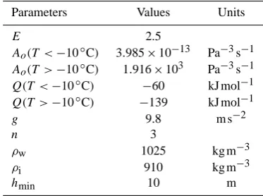
Table 1. List of parameter values used in this study.
Parameters Values Units
E 2.5
Ao(T <−10◦C) 3.985×10⁻¹³ Pa−3s−1 Ao(T >−10◦C) 1.916×10³ Pa−3s−1 Q(T <−10◦C) −60 kJ mol−1 Q(T >−10◦C) −139 kJ mol−1
g 9.8 m s−2
n 3
ρw 1025 kg m−3
ρi 910 kg m−3
hmin 10 m
ice-sheet volume is computed as the integral of the basis functions over the whole mesh. The ice discharge is com-puted as the ice flux through the lateral boundary0las D=
Z
0l
u.nd0. (9)
As the glaciated area (i.e. the area where ice thickness is larger thanhmin) can change with time, SMB is computed from Eq. (5) as
SMB=
Z
0s
(∂tzs+u∂xzs+v∂yzs−w)d0. (10)
Values of parameters prescribed in this study are pre-sented in Table 1. A proper initialisation of the tempera-ture field would require a spin-up over at least a full glacial cycle, which remains too computationally expensive with our model. In our application, the initial field is bi-linearly interpolated on the finite element mesh from the tempera-ture field computed with the shallow ice model SICOPO-LIS (Greve, 1997) after a paleo-climatic spin-up as in Sed-dik et al. (2012). In order to avoid an initialisation shock, as these two models do not have the same physics, the ice temperature field is then kept constant. The low conductivity of ice means that this assumption remains valid for the short time scales considered here. Because the ice-sheet basal tem-perature conditions remain uncertain, basal sliding is not re-stricted to areas where the ice temperature has reached the pressure melting point and an optimal friction coefficientβ
in Eq. (7) is inferred by inverse methods at each node to re-produce the observed surface velocity field (Sect. 3.1).
on a rough topography will depend on the choice of the im-plementation strategy. Using finite elements, the normals are uniquely defined element-by-element using the nodes coor-dinates and elemental shape functions. At a given node, the discontinuity of the normal direction to the elements sharing the node can be large if the typical length scale of the basal roughness is smaller than the mesh size.
The non-penetration condition (Eq. 7) can be enforced weakly by elements under the form of a Robin condition as n·(σ·n)|b+3u·n=0 (11) where3is an arbitrary large positive number. If the discon-tinuity of the normal direction,n, is large between adjacent elements, Eq. (11) will lead tou=0 at the node shared by such elements. Enforcing Eq. (7) as a Dirichlet condition im-plies a linear combination of the three components of the ve-locity vector in the general case wherenis not aligned with one of the coordinate axis. This can be done as in Leng et al. (2012) by using a local coordinate system with one direction aligned with the normal direction. A choice needs to be made on the definition of this normal direction as it is not uniquely defined, in general, at a given mesh node. The most immedi-ate possibility is to take the average of the normal direction to the elements sharing the node. The mass flux through an element, computed as the integral of the scalar product ofu withn, is then non null in general. This solution has been adopted in the following simulations. An alternative, newly implemented in the model, is to use mass consistent normals where the normal at a given node is a weighted average of the normal direction to the elements sharing the node. The weights are the nodal basis functions. This choice will insure that the zero-flux condition will be preserved globally, the non-null fluxes through the elements cancelling each other. However, it should be noted that this choice for the definition of the normal direction at the mesh nodes can be flawed with quadratic elements (Walkley et al., 2004).
2.2 Mesh construction
Anisotropic mesh adaptation is now widely used in numer-ical simulations especially with finite elements, as it allows to refine the mesh where needed to capture the flow features within a certain accuracy without increasing the computa-tional cost excessively. The method is generally based on an estimation of the interpolation error used to adjust the mesh size so that the discretisation error is equally distributed over the whole domain. It can be shown that an estimate of the interpolation error induced by the meshing is obtained from the Hessian matrix of the modelled field, allowing to define an anisotropic metric tensor at each node (Frey and Alauzet, 2005). As the target surface velocity field is known, our met-ric tensor is constructed from the Hessian matrix of observed surface speed (Joughin et al., 2010) shown in Fig. 1a. Start-ing from a first regular mesh of the 2-D footprint of the GrIS based on Delaunay triangulation, we use the freely
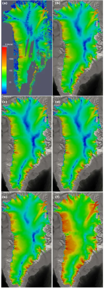
avail-Fig. 1. GrIS surface velocities. (a) Observed surface velocities
on the original regular 500 m×500 m grid; Computed surface
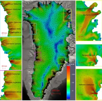
Fig. 2. Unstructured finite element mesh and model surface velocities after optimisation of the basal friction coefficient with the Robin
inverse method. Colored boxes show close-up views for various outlet glaciers of interest.
able anisotropic mesh adaptation software YAMS (Frey and Alauzet, 2005) to optimise the mesh sizes according to the given metric map.
The resulting mesh is depicted in Fig. 2. Mesh sizes de-crease from 40 km in the central part of the ice sheet to 1 km in the outlet glaciers. The 2-D mesh is then vertically ex-truded using 16 layers. The resulting 3-D mesh is composed of 417 248 nodes and 748 575 wedge elements.
The bedrock and surface topography are taken from the freely available SeaRise 1 km present-day data set (http://tinyurl.com/srise-umt) and are based on the Bamber et al. (2001) digital-elevation models where new data have been added on three of the main outlets (Jakobshavn Isbrae, Helheim and Kangerdlugssuaq). There is no freely available product for current ice margin position and the initial 2D-footprint has been constructed from a 0-m thickness contour.
3 Initial state
As ice-sheet responses include long time scales (multi-century), forecasting change on decadal-to-century time scales is essentially a short-term forecast. As such
computed in a diagnostic model is non-physical (Seroussi et al., 2011), and the available observations are not used here to constrain the model. The free surface is then allowed to relax compared to the observed surface for a period of 50 yr (Sect. 3.2). The performance of the model to simulate present-day conditions is then assessed by comparison of the estimated ice discharge for the main outlet glaciers (Rignot and Kanagaratnam, 2006).
3.1 Inverse methods
Two variational inverse methods (Arthern and Gudmunds-son, 2010; Morlighem et al., 2010) are used to infer the basal friction coefficient fieldβ(x, y). Both methods are based on the minimisation of a cost function that measures the mis-match between modelled and observed velocities. The two methods are briefly outlined below.
3.1.1 Robin inverse method
The method, detailed in Arthern and Gudmundsson (2010), consists in solving alternatively the Neumann-type problem, defined by Eq. (4) and the boundary conditions in Eqs. (6) and (7), and the associated Dirichlet-type problem, defined by the same equations except that the Neumann upper-surface condition (Eq. 6) is replaced by a Dirichlet condition where observed surface horizontal velocities are imposed.
The cost function that expresses the mismatch between the solutions of the two models is given by
Jo=
Z
0s
(uN−uD)·(σN−σD)·nd0, (12)
where superscripts N and D refer to the Neumann and Dirich-let problem solutions, respectively.
The Gˆateaux derivativedβJoof the cost functionJowith
respect to the basal friction coefficientβ for a perturbation
β0is given by
dβJo=
Z
0b
β0(|uD|2− |uN|2)d0, (13)
where the symbol|.|defines the norm of the velocity vector and0bis the lower surface.
Note that this derivative is exact only for a linear rheology and thus Eq. (13) is only an approximation of the true deriva-tive of the cost function when using Glen’s flow law (Eq. 1) withn >1 in Eq. (2).
3.1.2 Control inverse method
The control method has been introduced by MacAyeal (1993) and recently applied to full-Stokes ice flow modelling by Morlighem et al. (2010). The method relies on the compu-tation of the adjoint of the Stokes system. As in Morlighem et al. (2010), we assume that the stiffness matrix of the Stokes
system is independent of the velocity and thus self adjoint, which is valid only for Newtonian rheology, i.e. whenn=1 in Eq. (2).
As the direction of the ice velocity is mainly governed by the ice-sheet topography, we disregard the error on the veloc-ity direction and the cost function is expressed as the differ-ence between the norm of the modelled and observed hori-zontal velocities as
Jo= Z 0s 1 2
|uH| − |uobsH |
2
d0, (14)
whereuobsare the observed velocities and subscriptHrefers to the horizontal component of the velocity vector.
The Gˆateaux derivative is obtained by dβJo=
Z
0b
−β0u·λd0, (15)
whereλis the solution of the adjoint system of the Stokes equations.
Again, this derivative is exact only for a linear rheology and thus is only an approximation of the true derivative of the cost function when using Glen’s flow law (Eq. 1) with
n >1 in Eq. (2). 3.1.3 Regularisation
To avoid non-physical negative values of the basal friction coefficient,βis expressed as
β=10α. (16)
The optimisation is now done with respect to α and the Gˆateaux derivative ofJowith respect toαis written as dαJo=dβJo
dβ
dα. (17)
To avoid over fitting of the data and improve the condi-tioning of the problem, a smoothness constraint is added to the cost function under the form of a Tikhonov regularisation term penalising the spatial first derivatives ofαas
Jreg= 1 2 Z 0b ∂α ∂x 2 + ∂α ∂y 2
d0. (18)
The Gˆateaux derivative ofJregwith respect toαfor a pertur-bationα0is obtained by
dαJreg=
Z 0b ∂α ∂x ∂α0 ∂x + ∂α ∂y ∂α0 ∂y
d0. (19)
The total cost function is now written as
Jtot=Jo+λJreg, (20)
2.6e+16 2.8e+16 3e+16 3.2e+16 3.4e+16 Jo
1 10 100 1000 10000 1e+05
2.5e+12 5e+12 7.5e+12 1e+13
Jo 1
10 100 1000 10000 1e+05
Jreg
λ=0.0
λ=108
λ=1010
λ=1011
λ=1012
λ=1013
λ=1014
λ=1010
λ=1012
λ=109
λ=108
λ=107
λ=106
λ=0
λ=1011
Robin inverse method Control inverse method
Fig. 3. L-Curve obtained with the Robin (left) and Control (right) inverse methods.
3.1.4 Minimisation
Surface ice flow speeds vary over several order of magni-tudes between the interior of the ice sheet (slow flow) and the outlet glaciers (fast flow). Therefore, Sch¨afer et al. (2012) have shown that good convergence properties are obtained with the Robin inverse method by using a spatially varying step size rather than the fixed-step used in the original gradi-ent descgradi-ent algorithm of Arthern and Gudmundsson (2010). We apply here another strategy where the Gˆateaux deriva-tives given by a continuous scalar product represented by the integral on0b, Eqs. (17) and (19), are transformed in a dis-crete euclidean product when discretized on the finite ele-ment mesh. The area surrounding each finite eleele-ment node on0bis then included in the gradients used for the minimi-sation. This leads to good convergence properties with our unstructured mesh as large elements correspond to low ve-locity areas, and vice versa.
The minimisation of the cost function Jtot with respect toα is done using the limited memory quasi-Newton rou-tine M1QN3 (Gilbert and Lemar´echal, 1989) implemented in Elmer in reverse communication mode. This method uses an approximation of the second derivatives of the cost function and is then more efficient than a fixed-step gradient descent. 3.1.5 Results
The observed velocities, shown in Fig. 1a, are a compila-tion of data sets obtained from RADARSAT data at differ-ent dates during the first decade of the 2000s (Joughin et al., 2010). We choose this compilation as it gives the best cov-erage. For glaciers that have been accelerating, it therefore provides a kind of average value for this period. But for these glaciers, the surface topography has also diverged from the surface topography used here. A proper comparison of the model results with observations of the 2000s would therefore require coherent data sets for both the topography and the ve-locities, which are currently not available. For the inversion,
gaps in data have been filled by the balance velocities avail-able in the SeaRise data set. As these gaps are mainly located in areas of low speed in the central parts of the ice sheet, ex-cept in the south and south-east, no special care has been taken to insure continuity between balance and observed ve-locities.
To compare the performance of the two inverse methods and assess the dependence of the results to the initialisation of the basal friction coefficientβ, the initial field is given by
β(x, y)=max(10−4,min(1.0/Ubal,10−1))MPa m−1a (21) for the Robin inverse method whereUbalis the balance ve-locity, and by
β(x, y)=10−4MPa m−1a (22)
for the control inverse method.
The optimal regularisation parameterλin Eq. (20) is cho-sen using the L-curve method (Hancho-sen, 2001). The L-curve is a plot of the optimised variable smoothness, i.e. the term
Jregin Eq. (20), as a function of the mismatch between the model and the observations, i.e. the termJoin Eq. (20). The
L-curve obtained with both methods is given in Fig. 3. The termJregis identical for the two methods, whereasJois not
(Eqs. 12 and 14). This leads to different values of the regu-larisation parameterλ in Eq. (20), which allows tuning the weight of the regularisation with respect toJo.
For the Robin inverse method, when increasingλfrom 0 to 109, the roughness of the basal friction coefficient field, represented byJreg, decreases by several orders of magnitude with a small decrease of the mismatch between the model and the observation, represented byJo. This decrease ofJo
may be due to the fact that the gradient used in the model, Eq. (13), is not the true gradient ofJodue to the nonlinearity
of the ice rheology. The regularisation, for which the gradient is exact, therefore improves the convergence properties of the model. For higher values ofλ,Jreg still decreases but with a concomitant increase ofJoas the basal friction coefficient
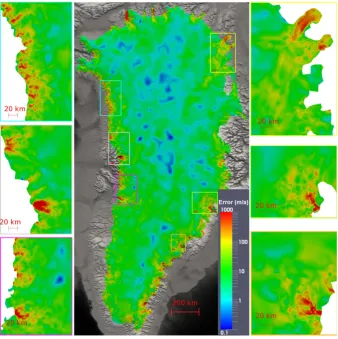
Fig. 4. Absolute error on surface velocities|umod−uobs|in m a−1at the end of the optimisation using the Robin inverse method.
The L-curves obtained with the two methods are very sim-ilar. The minimumJois obtained for the same order of mag-nitude ofJreg. The optimal value forλis chosen as the min-imum value ofJo, i.e. λRobin=108 for the Robin inverse method, andλCI=1011for the control inverse method.
The surface velocity field obtained after optimisation of the basal friction coefficient field with the Robin inverse method is shown in Fig. 2. Our implementation reproduces very well the observed large-scale flow features (Fig. 1a) with low velocities in the interior and areas of rapid ice flow, restricted to the observed outlet glaciers, near the mar-gins. The largest outlet glaciers (Jakobshavn Isbrae, Kanger-lugssuaq, Helheim, . . . ) and their catchments are well cap-tured by the anisotropic mesh and the modelled velocity pat-tern is in good agreement with the observations. Smaller out-let glaciers down to a few kilometres in width are also indi-vidually distinguishable.
The absolute and relative errors on the surface velocities at the end of the optimisation are shown in Figs. 4 and 5, respectively. Similar to the velocity magnitude, the absolute error varies by several orders of magnitude between the in-terior and the margins. The relative error is only few per-cents in most of the interior where ice is flowing faster than
few meters per year. This error is usually higher very locally near the margins. The highest relative errors are located in the North in Petermann Glacier and in the Northeast Greenland Ice Stream where long floating tongues are present but not explicitly taken into account in this application of the model. The remaining differences between modelled and observed velocities can come from four main reasons:
i. non convergence of the minimisation: it has been shown on twin experiments where the minimum is known (Arthern and Gudmundsson, 2010) that the gradients of the cost function derived analytically for a linear rheology, Eqs. (13) and (15), work well in practice with a non-linear rheology. But there is no guarantee that the actual minimum will be found (Goldberg and Sergienko, 2011), especially in real applications where the curvature of the cost function is very low.
Fig. 5. Relative error on surface velocities|umod−uobs|/|uobs|in % at the end of the optimisation using the Robin inverse method. Areas
where|uobs|<2.5 m a−1have been removed from display.
iii. Too coarse spatial resolution of the model where the minimum mesh resolution is lower than those of the ve-locity data, so that the model will not be able to capture all details, especially for the smallest outlets;
iv. Too coarse spatial resolution of the data as, for example, the ice thickness is not sufficiently known in most outlet glaciers.
It is difficult to test the first hypothesis as the minimum is un-known but both the cost function and the norm of the gradient decrease during the minimisation and both inverse methods lead to very similar results (not shown for the control inverse methods), so that we are confident to be close to the actual minimum.
Errors shown in Figs. 4 and 5 account both for the error on the direction and on the magnitude of the modelled veloc-ities compared to the observations. The direction of the flow is mainly governed by the ice-sheet topography and adjusting the sliding coefficient has little effect on the flow direction. The cost function used with the control inverse method only accounts for the difference between the velocity norms and not for the direction. Both inverse methods lead to similar
errors so that we assume that most of the absolute error is representative of the error on the velocity norm. For the out-lets, a common feature is that model velocities are lower than the observations along the central flow lines but higher along the shear margins (not shown here). This can be explained by insufficient resolution of the model and/or of the data, or remaining uncertainties on the ice viscosity for example. 3.2 Relaxation
When running prognostic simulations from this initialisation, the free-surface elevation shows non-physical rates of change especially at the margins (Fig. 6). The free surface of the ice sheet is therefore allowed to relax during a 50-yr time-dependent run, forced by a constant present-day surface mass balance field (Ettema et al., 2009).
Fig. 6. Free surface elevation absolute rate of change: (a) after 1 yr
of relaxation; (b) after 50 yr of relaxation.
glaciers are not able to evacuate the ice flowing through them and they need to thicken up. One explanation is that the ice thicknesses of many outlet glaciers is poorly known and they may be thicker in reality than the current geometry data al-lows for. The other explanation is that the lateral side of the mesh does not correspond exactly to the current position of the fronts of marine terminating glaciers for which we have no compilation for the whole GrIS. The ice then needs to be transported towards the edge of the domain to be evac-uated as discharge through the lateral boundary. This effect can be shown on the results for the ice discharge globally (Fig. 7) and locally for individual outlet glaciers (Table 2). Ice discharge is very low and underestimated for most of the smallest outlet glaciers at the beginning of the relaxation but increases with time as ice reaches the edges of the domain.
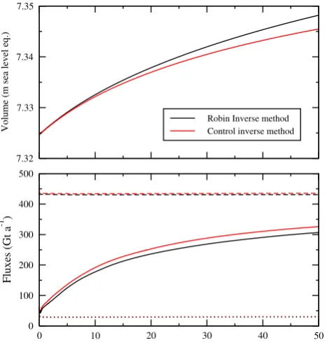
The time needed to offset these uncertainties and reach an equilibrium is difficult to estimate in advance and will be dif-ferent for each drainage basin. The relaxation duration is ar-bitrarily fixed to 50 years. At the end of the relaxation, the surface velocity structure, given in Fig. 1b, remains similar to the observations, with rapid ice flow areas still concentrated in known outlet glaciers. The various terms of the mass bal-ance equation during the relaxation are given in Fig. 7. SMB is nearly constant and equal to 430 Gt a−1during the relax-ation showing that the glaciated area has not changed dra-matically. Most of the ice discharge increase happen during the first twenty years to reach 200 Gt a−1, after this increase slows down. During this relaxation the ice volume increases by less than 0.5 %. Running the model longer should lead to a steady state where the ice discharge should offset the
sur-Table 2. Model discharge for individual outlets and the whole ice
sheet in Gt a−1: after 1 yr (RI 1a) and after 50 yr (RI 50a) of
sur-face relaxation with the Robin inverse method, after 50 yr of sursur-face relaxation with the control inverse method (CI 50a), and observa-tions from 1996 (or 2000 when not available, and converted from
km3a−1to Gt a−1using a uniform density of 910 kg m−3for ice)
(Rignot and Kanagaratnam, 2006) (Obs.).
RI 1a RI 50a CI 50a Obs.
West
Jakobshavn I. 30.2 24.4 26.1 21.5
Sermeq kujatd 0.4 7.8 7.9 9.1
Rink 13.8 9.7 10.5 10.7
Hayes 0.1 4.1 3.7 9.0
East
Daugaard-Jensen 0.0 7.2 7.4 9.1
Kangerdlugssuaq 0.1 9.9 11.1 25.3
Helheim 10.3 23.7 24.0 23.9
Ikertivaq 0.2 22.5 22.8 9.2
North
Petermann 0.0 1.9 4.0 10.7
Nioghalvfjerdsbrae 0.0 4.5 4.6 12.3
Zachariae I. 0.5 6.7 7.0 9.0
Total 65.1 306.7 326.0 325
face mass balance as shown in Fig. 8 when running the same constant climatic scenario for another century.
At the end of the relaxation, the rate of increase of the ice discharge is around 1 Gt a−2and the free surface is nearly at equilibrium except in a few areas near the margins. As shown by Fig. 9a when running the same scenario for another 10 years, this remaining elevation change is mainly positive as these areas are still unable to evacuate all the ice flowing to them but the rate of change is within a physically acceptable range (Fig. 6). The change in surface elevation between the beginning and the end of the relaxation exceeds several hun-dred meters in some places. This difference is large but is of the same order of magnitude as the uncertainty on the ice thickness in some areas of the GrIS margins. This remains the main limitation of the model where only the upper sur-face is adjusted to compensate the remaining uncertainties in the model initial conditions.
7.32 7.33 7.34 7.35
Volume (m sea level eq.)
Robin Inverse method Control inverse method
0 10 20 30 40 50
0 100 200 300 400 500
Fluxes (Gt a
-1 )
Fig. 7. GrIS mass balance during relaxation: (top) evolution of the
total ice volume in meters of sea level equivalent and (bottom) evo-lution of the discharge (solid lines), SMB (dashed lines) and flux
through the bedrock (dotted lines) in Gt a−1.
Kandgerdlugssuaq where the drainage basin still shows high rates of surface-elevation change (Fig. 6). Discharge at Pe-termann Glacier and the Northeast Greenland Ice Stream is also largely underestimated by up to 80 % and these glaciers are still thickening at high rates. This can be explained by the fact that their floating tongues are not treated explicitly in the model resulting in the neglect of the mass loss from melt-ing below the shelves at the interface with the ocean. The total computed discharge for the relaxed solution is around 300 Gt a−1. Up to now, the magnitude of the computed ice discharge in a continental ice-sheet model has only been ad-dressed by Price et al. (2011) by tuning the boundary con-dition at the ice front to reproduce the observations only on three major outlets.
The evolution of the total volume and ice discharge ob-tained with the basal friction coefficient field optimised with the two inverse methods are very similar. This is true for each individual outlet as shown in Table 2. The two inverse meth-ods perform similarly and neither can be favoured in view of these results or in terms of computation performance.
4 Sensitivity experiments
We use the relaxed solution of the Robin inverse method as the starting point to investigate the GrIS mass balance over one century.
Table 3. Model discharge for individual outlets and the whole ice
sheet in Gt a−1after one century for the various experiments.
C1 BF1 C2 BF1 C2 BF2 C2 BF3
West
Jakobshavn I. 22.7 16.9 27.2 108.5
Sermeq kujatd. 8.5 3.8 8.8 48.3
Rink 10.6 9.9 13.8 31.4
Hayes 4.7 2.3 5.1 26.0
East
Daugaard-Jensen 8.0 9.0 12.8 35.9
Kangerdlugssuaq 11.8 11.5 16.4 47.0
Helheim 24.9 23.8 30.6 82.6
Ikertivaq 24.3 20.3 24.7 59.6
North
Petermann 5.8 1.1 5.4 34.9
Nioghalvfjerdsbrae 6.6 4.8 11.6 58.2
Zachariae I. 7.5 6.1 13.7 66.3
Total 362.7 252.4 387.1 1404.5
4.1 Set up
The climate forcing in the model impacts ice dynamics only through the net accumulation rate at each surface mesh node as the ice temperature field is kept constant. Two SMB sce-narios are used, the first (C1), corresponds to keeping present conditions (Ettema et al., 2009) constant with time; the sec-ond (C2) represents an ensemble of 18 climate models forced under the IPCC A1B emission scenario. These forcings are taken from the freely available SeaRISE data compilations (http://tinyurl.com/srise-umt).
Here, we especially focus on the GrIS dynamical response to an increase in basal lubrication. Perturbations are intro-duced by applying three homogeneous changes in the basal friction coefficientβ from the initial fieldβi(x, y) inferred
by the inverse method (Sec. 3.1).
i. No perturbation withβunchanged form the initial field (BF1):
β(x, y, t )=βi(x, y) ∀x, y, t. (23)
ii. A constant perturbation, introduced as a step function, withβdivided by two and then kept constant (BF2):
β(x, y, t )=1
2βi(x, y) ∀x, y, t. (24)
iii. A continuously enhanced perturbation withβ reduced by one order of magnitude over one century (BF3):
α(x, y, t )=αi(x, y)−t /100 ∀x, y, (25)
wheret is the simulation time (0≤t≤100) andβ=
magnitude with only small changes in the water pres-sure so that the magnitude of the imposed changed would not be unrealistic if applied in few locations and for short time periods. However, it seems highly un-likely that the GrIS will surge all at the same time, so that this last sensitivity experiment is used as an high end scenario of the possible future for the GrIS mass loss.
Further destabilisations introduced by changes in the sea-ward boundary conditions or weakening of the lateral mar-gins are excluded from this study. Experiments are hereafter referred to by the climate forcing (C1 or C2) and the basal friction scenario (BF1, BF2 or BF3).
4.2 Results
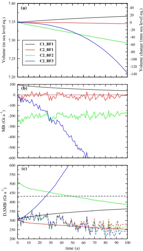
We evaluate the results of the perturbations by considering ice-flow velocities (Fig. 1), the ice-sheet total mass balance (Fig. 8), discharge values from the main outlet glaciers (Ta-ble 3) and free-surface-elevation rate-of-change (Fig. 9). For the ice-sheet total mass balance (Fig. 8), we present the total ice-sheet volume and volume change from the starting point, converted to sea-level equivalents (Fig. 8a). The annual mass balance (MB, Fig. 8b) is obtained as the time derivative of the ice-sheet volume, and the respective contributions of D and SMB are given in Fig. 8c. The difference between MB and SMB-D is the ice flux lost through the bottom boundary (see Sect. 2.1, discussion on boundary condition Eq. 7). In all the applications it corresponds approximately to 10 % of D.
With constant conditions (C1 BF1), the model tends to reach a steady state where the modelled discharge balances the current SMB (430 Gt a−1, Fig. 8c). Neither the glaciated area, nor the surface velocity pattern, change dramatically during this experiment (Fig. 1c) and the ice discharge shows a small increase in the main outlets (Table 3).
The climatic perturbation used here (SMB scenario C2) shows a reduction of SMB of approximately only 100 Gt a−1 after one century (Fig. 8c), which is a lower bound of the forecast given by current climate models (Fettweis et al., 2008). Changes in the glaciated area between the three per-turbation experiments detailed below lead to only small dif-ferences in the total SMB after one century (Fig. 8c). These differences are one order of magnitude lower than those be-tween the various climate models (Fettweis et al., 2008) but do not account for the possible feedback between the ice-sheet topography and climate as the prescribed accumula-tion is only a funcaccumula-tion of posiaccumula-tion and time. Investigating this feedback requires proper coupling of high resolution ice-sheet and climate models.
Without dynamic perturbation (C2 BF1), the computed ice discharge is of the same order of magnitude as the SMB and decreases at an equivalent rate (Fig. 8c). The resulting annual mass balance is nearly centred around zero and lacks a particular trend over the century (Fig. 8b), as a consequence,
7.20 7.25 7.30 7.35 7.40
Volume (m sea level eq.)
C1_BF1 C2_BF1 C2_BF2 C2_BF3
0 10 20 30 40 50 60 70 80 90 100
time (a) 200
250 300 350 400 450 500 550 600
D,SMB (Gt a
-1 )
-600 -500 -400 -300 -200 -100 0 100
MB (Gt a
-1 )
-140 -120 -100 -80 -60 -40 -20 0 20 40
Volume change (mm sea level eq.)
(a)
(b)
(c)
Fig. 8. GrIS future mass balance as a function of time: (a) total ice
volume (left axis, meters of sea level equivalent) or volume change from initial time (right axis, milimeters of sea level equivalent), (b) annual mass balance (the brown line correspond to 0) and (c)
dis-charge (D) (solid lines) and SMB (dashed lines) in Gt a−1.
the total ice volume is nearly constant (Fig. 8a). For this ex-periment, the velocity pattern (Fig. 1d) remains similar to the present one. The increase of ablation for this climate sce-nario is higher in West Greenland. This leads to thinning of the marginal ice in this area, resulting in a retreat of land ter-minating glaciers and in a decrease in ice discharge of marine terminating glaciers (Table 3).
With a constant dynamic perturbation (C2 BF2), halving
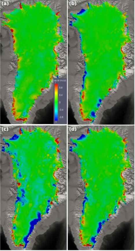
Fig. 9. Free surface elevation rate of change after 10 yr for
experi-ments (a) C1 BF1, (b) C2 BF1, (c) C2 BF2, and (d) C2 BF3.
based on observations (Rignot et al., 2011). However, this is done at the expense of the velocity pattern as we see higher velocities on the interior of each drainage basin (Fig. 1e) compared to the current observations (Fig. 1a). A progres-sion of high velocitie areas upstream of each drainage basin may be expected as ablation will reach higher elevations in the future, increasing water pressure and basal lubrications in these areas. However, the expected effect in low elevation areas is not clear as the increase of water availability should contribute in the formation of efficient drainage systems re-sulting in a decrease of the water pressure and basal lubri-cation (Schoof, 2010). With this experiment, we investigate how an initial ice-sheet imbalance of−200 Gt a−1, which is
close to the current observations, can evolve within a century. The computed total discharge decreases throughout the 100-yr simulation at a rate equivalent to the rate of decrease of SMB except during the first decade where it decreases faster probably as a reaction to the initial perturbation (Fig. 8c). As a result, after the first decade the annual mass balance shows no particular trend (Fig. 8b) and the ice sheet loses mass at a nearly constant rate throughout the century (Fig. 8a). With this experiment, the retreat of land terminating glaciers in the west coast induced by the increase of ablation is com-pensated by their acceleration, allowing to drain more ice to the areas subjected to high ablation. Again, the reduction of the discharge throughout the simulation is higher in the west coast as more ice is melted before reaching the margins of the domain.
With an increasing dynamic perturbation (C2 BF3), the discharge increases continuously from 300 Gt a−1 to 1400 Gt a−1after 100 yr (Fig. 8c), and the ice sheet is los-ing mass throughout the 100-yr simulation (Fig. 8a, b). With this result we show that the acceleration of the ice discharge observed during the last decade (Rignot et al., 2011) can be maintained over a whole century. However, the velocity pat-tern at the end of the century (Fig. 1f), shows large areas of high velocities (>100 m a−1) far inland of each glacier. Such a scenario seems unlikely as it would required a sustained surge of the whole ice sheet in the same time, which is ex-cluded if efficient drainage systems develop as a result of in-creased water supply (Schoof, 2010). As a consequence, we estimate that, in the absence of further destabilisation of the GrIS ocean margins, this scenario represents an upper bound for the ice-sheet contribution to SLR by 2100.
An important output of these experiments is that the ice discharge shows an extremely rapid adjustment to perturba-tions as shown at the beginning of the relaxation (Fig. 7b) and in response to the dynamical perturbations (for both ex-periments BF2 and BF3, Fig. 8c). However, the spatial and temporal variability of the forcings affecting the basal and seaward boundary conditions of the ice sheet remain poorly constrained, limiting the forecast ability of the models.
With experiment C1 BF1, as discussed previously, some drainage basins are still not at equilibrium and their out-lets are still thickening due to a SMB higher than the com-puted discharge. In the interior, the surface elevation change is nearly zero. With a climate perturbation only, i.e. exper-iment C2 BF1, the margins in the west and south-east are thinning and the thickening of Petermann Glacier and the Northeast Greenland Ice Stream is less pronounced. These differences with experiment C1 BF1 mostly come from the change in the SMB term.
Experiments with a dynamical perturbation, i.e C2 BF2 and C2 BF3, show an additional dynamical thinning asso-ciated with the acceleration of the ice, upstream of each drainage basin. Downstream, near the margins, this gives two different behaviours. (i) If the decrease of the basal fric-tion coefficient also produces an accelerafric-tion and an increase of the discharge sufficient to offset the mass excess coming from upstream, the whole ice stream shows a dynamical thin-ning. This is the case in the south-east and for Jakobshavn Isbrae and Heilhem Glacier. (ii) If the acceleration and the increase of ice discharge are not sufficient, this results in a dynamical thickening of the margins. This is the case in the north-west and for Kangerdlussuaq Glacier. For land ter-minating glaciers south of Jakobsahvn Isbrae, the thinning induced by the increase of ablation is partly offset by this dynamical thickening.
In some aspects, these results therefore agree with obser-vations and show an interesting regional variability of the re-sponse to the dynamical perturbation. The link between sur-face runoff, basal hydrology and basal sliding will have to be investigated more in-depth to make quantitative compar-isons.
5 Conclusions
We have shown that our implementation of a model with the correct treatment of longitudinal stresses, sufficient resolu-tion to resolve medium to small outlet glaciers, and a care-ful initialisation of ice-flow parameters allows us to satisfy the essential prerequisite of simulating the observed velocity structure of the ice sheet. Neither of the two recent inverse methods used to infer the basal friction coefficient field from the knowledge of the ice-sheet topography and ice-surface velocities can be favoured in view of our results.
Due to the remaining uncertainties in the model initial conditions, the ice-sheet surface has been allowed to diverge from the observations during a relaxation period of 50 years. This is the main limitation of the model as this relaxation drives the model towards a steady state, limiting our ability to capture the currently observed transient response of the GrIS. However, we have shown that, after the relaxation, the ice discharge obtained globally and for individual outlet glaciers is still in good agreement with observations of the late 1990s. The main remaining uncertainties in the model are the ice
viscosity field, the bedrock elevation and the position of the ice margins. Future work will benefit from new observations and from the developments of inverse methods to constrain these uncertainties (Arthern and Gudmundsson, 2010; Pra-long and Gudmundsson, 2011; Morlighem et al., 2010; Petra et al., 2012). However, these methods remain restricted to di-agnostic simulations and proper methods, such as automatic differentiation of the true discrete adjoint model (Heimbach and Bugnion, 2009), still have to be applied to higher-order ice flow modelling to capture the observed transient response of the ice sheet.
More specific projections will arise as the ice sheet is driven by more complete and precise climate scenarios, and with greater understanding of processes at the front of out-let glaciers. Our new-generation continental-scale ice-sheet model is well suited to incorporate such information as it becomes available. However, our current model experiments are significant and general conclusions can already be drawn. Results confirms that the overall mass balance of the GrIS is sensitive, not only to changing SMB, but in large parts, to ice discharge. Our model shows a rapid adjustment of the ice discharge in response to dynamical perturbations. This is supported by other models that include processes at the ice front (Nick et al., 2009, 2012) and by recent observations (Howat et al., 2007). Moving ice margins and a physically based treatment of calving are essential future developments of the model, and are required to move from sensitivity ex-periments to realistic projections of the ice discharge evolu-tion.
Results show that, unless the perturbation is continuously enhanced, an increase of the surface ablation reduces the dis-charge, stabilising the ice sheet. However, this effect could be negated if the thinning of outlet glaciers results in fur-ther destabilisation and retreat of the ocean margins making it possible to sustain high discharge rates. Nevertheless, this demonstrates that, even on a century timescale, discharge and surface mass balance anomalies cannot be treated indepen-dently in estimating the GrIS contribution to SLR. This effect could be even higher due to the possible feedback between surface elevation and surface mass balance. Proper coupling with local surface mass balance models will then be required to improve the model predictive ability.
We use the modelling conducted here and the currently observed ice-sheet mass balance to estimate possible bounds for the future GrIS contribution to SLR. These bounds do not take into account possible further movements of the GrIS ocean margins as proper treatment of the processes affecting their stability in a whole ice-sheet model is still lacking.
balance in 2010 (Rignot et al., 2011) leads to a total contri-bution to SLR of 75 mm by 2100. This value is comparable to the 46 mm (40 mm from SMB and 6 mm from dynamics) given by Price et al. (2011) as an estimate of the committed SLR due to the observed last decade ice-sheet dynamics. Our value is closer to their estimated upper bound (85 mm includ-ing 45 mm from dynamics) which is estimated by assuminclud-ing a self-similar response of the ice sheet to a 10 yr-recurring forcing in the future decades (Price et al., 2011) .
We have shown that, conversely, if the forcing is contin-uously increased, there is sufficient ice available to sustain the current rate of increase in discharge over an entire cen-tury. However, in our model, this is achieved by a very strong perturbation of the basal lubrication field. Under these condi-tions, a probable upper bound for the ice-sheet contribution to SLR is given by assuming that this rate of increase will be preserved in the future. Taking a discharge anomaly of 100 Gt a−1increasing at rate of 9 Gt a−2for year 2010 (Rig-not et al., 2011), leads to a contribution to SLR of 140 mm by 2100 from dynamics only. This value is in the lower half of the values obtained from kinematic considerations assum-ing low (93 mm) and high (467 mm) scenarios (Pfeffer et al., 2008).
Acknowledgements. We would like to thank Jesse Johnson and two anonymous referees for their helpful comments on the manuscript. This work was supported by both the ice2sea project funded by the European Commission’s 7th Framework Programme through grant number 226375 (Ice2sea contribution number ice2sea052) and the ADAGe project (ANR-09-SYSC-001) funded by the Agence National de la Recherche (ANR). Hakime Seddik and Ralf Greve were supported by a Grant-in-Aid for Scientific Research A (No. 22244058) from the Japan Society for the Promotion of Sci-ence (JSPS). We thank I. Joughin for providing the surface velocity data and the SeaRISE community (http://tinyurl.com/srise-umt) for the compilation of topography and climate forcing data sets. We also thank J. Ruokolainen and P. R˚aback for their continuous support in developing Elmer. This work was performed using HPC resources from GENCI-CINES (Grant/2011016066/) and from the Service Commun de Calcul Intensif de l’Observatoire de Grenoble (SCCI).
Edited by: I. M. Howat
The publication of this article is financed by CNRS-INSU.
References
Alley, R. B. and Joughin, I.: Modeling ice-sheet flow, Science, 336, 551–552, doi:10.1126/science.1220530, 2012.
Arthern, R. J. and Gudmundsson, G. H.: Initialization of ice-sheet forecasts viewed as an inverse Robin problem, J. Glaciol., 56, 527–533, 2010.
Bamber, J. L., Layberry, R. L., and Gogineni, S. P.: A new ice thick-ness and bed data set for the Greenland ice sheet 1. Measurement, data reduction, and errors, J. Geophys. Res., 106, 33773–33780, 2001.
Ettema, J., van den Broeke, M. R., van Meijgaard, E., van de Berg, W. J., Bamber, J. L., Box, J. E., and Bales, R. C.: Higher surface mass balance of the Greenland ice sheet revealed by high-resolution climate modeling, Geophys. Res. Lett., 36, L12501, doi:10.1029/2009GL038110, 2009.
Favier, L., Gagliardini, O., Durand, G., and Zwinger, T.: A three-dimensional full Stokes model of the grounding line dynamics: effect of a pinning point beneath the ice shelf, The Cryosphere, 6, 101–112, doi:10.5194/tc-6-101-2012, 2012.
Fettweis, X., Hanna, E., Gall´ee, H., Huybrechts, P., and Er-picum, M.: Estimation of the Greenland ice sheet surface mass balance for the 20th and 21st centuries, The Cryosphere, 2, 117– 129, doi:10.5194/tc-2-117-2008, 2008.
Frey, P. and Alauzet, F.: Anisotropic mesh adaptation for CFD computations, Comput. Method Appl. M., 194, 5068–5082, doi:10.1016/j.cma.2004.11.025, 2005.
Gagliardini, O. and Zwinger, T., The ISMIP-HOM benchmark ex-periments performed using the Finite-Element code Elmer, The Cryosphere, 2, 67–76, 2008,
http://www.the-cryosphere-discuss.net/2/67/2008/.
Gilbert, J. C. and Lemar´echal, C.: Some numerical experiments with variable-storage quasi-Newton algorithms, Math. Program., 45, 407–435, doi:10.1007/BF01589113, 1989.
Glen, J. W.: The creep of polycrystalline ice, P. Roy. Soc. Lond. A Mat., 228, 519–538, doi:10.1098/rspa.1955.0066, 1955. Goldberg, D. N. and Sergienko, O. V.: Data assimilation
us-ing a hybrid ice flow model, The Cryosphere, 5, 315–327, doi:10.5194/tc-5-315-2011, 2011.
Greve, R.: Application of a polythermal three-dimensional ice sheet model to the Greenland ice sheet: response to steady-state and transient climate scenarios, J. Climate, 10, 901–918, 1997. Greve, R. and Blatter, H.: Dynamics of Ice Sheets and Glaciers,
Springer, Berlin, Germany etc., doi:10.1007/978-3-642-03415-2, 2009.
Hansen, P.: The L-curve and its use in the numerical treatment of inverse problems, Computational inverse problems in electrocar-diology, 5, 119–142, 2001.
Heimbach, P. and Bugnion, V., Greenland ice-sheet volume sensitiv-ity to basal, surface and initial conditions derived from an adjoint model, Annals Glaciol., 50(52), 67–80, 2009.
Howat, I. M., Joughin, I., and Scambos, T. A.: Rapid changes in ice discharge from Greenland outlet glaciers, science, 315, 1559– 1561, doi:10.1126/science.1138478, 2007.
Jay-Allemand, M., Gillet-Chaulet, F., Gagliardini, O., and Nodet, M.: Investigating changes in basal conditions of Var-iegated Glacier prior to and during its 1982–1983 surge, The Cryosphere, 5, 659–672, doi:10.5194/tc-5-659-2011, 2011. Joughin, I., Smith, B. E., Howat, I. M., Scambos, T., and Moon, T.:
map-ping, J. Glaciol., 56, 415–430, 2010.
Larour, E., Seroussi, H., Morlighem, M. and Rignot, E., Continental scale, high order, high spatial resolution, ice sheet modeling us-ing the Ice Sheet System Model, J. Geophys. Res., 117, F01022, doi:10.1029/2011JF002140, 2012.
Leng, W., Ju, L., Gunzburger, M., Price, S., and Ringler, T.: A par-allel high-order accurate finite element Stokes ice sheet model, J. Geophys. Res., 117, F01001, doi:10.1029/2011JF001962, 2012. Little, C. M., Oppenheimer, M., Alley, R. B., Balaji, V., Clarke, G. K. C., Delworth, T. L., Hallberg, R., Holland, D. M., Hulbe, C. L., Jacobs, S., Johnson, J. V., Levy, H., Lip-scomb, W. H., Marshall, S. J., Parizek, B. R., Payne, A. J., Schmidt, G. A., Stouffer, R. J., Vaughan, D. G., and Winton, M.: Toward a new generation of ice sheet models, Eos, 88, 578, doi:10.1029/2007EO520002, 2007.
MacAyeal, D. R.: A tutorial on the use of control methods in ice-sheet modeling, J. Glaciol., 39, 91–98, 1993.
Moon, T., Joughin, I., Smith, B., and Howat, I.: 21st-century evo-lution of Greenland outlet glacier velocities, Science, 336, 576– 578, doi:10.1126/science.1219985, 2012.
Morlighem, M., Rignot, E., Seroussi, H., Larour, E., Dhia, H. B., and Aubry, D.: Spatial patterns of basal drag inferred using con-trol methods from a full-Stokes and simpler models for Pine Island Glacier, West Antarctica, Geophys. Res. Lett., 37, 6, doi:10.1029/2007EO520002, 2010.
Morlighem, M., Rignot, E., Seroussi, H., Larour, E., Dhia, H. B., and Aubry, D.: A mass conservation approach for map-ping glacier ice thickness, Geophys. Res. Lett., 38, L19503, doi:10.1029/2011GL048659, 2011
Nick, F. M., Vieli, A., Howat, I. M., and Joughin, I.: Large-scale changes in Greenland outlet glacier dynamics triggered at the ter-minus, Nat. Geosci., 2, 110–114, doi:10.1038/NGEO394, 2009 Nick, F. M., Luckman, A., Vieli, A., Van der Veen, C. J., Van
As, D., Van de Wal, R. S. W., Pattyn, F., Hubbard, A. L. and Floricioiu, D.: The response of Petermann Glacier, Greenland, to large calving events, and its future stability in the context of at-mospheric and oceanic warming, J. Glaciol., 58(208), 229–239, 2012.
Pattyn, F., Perichon, L., Aschwanden, A., Breuer, B., de Smedt, B., Gagliardini, O., Gudmundsson, G. H., Hindmarsh, R. C. A., Hubbard, A., Johnson, J. V., Kleiner, T., Konovalov, Y., Mar-tin, C., Payne, A. J., Pollard, D., Price, S., R¨uckamp, M., Saito, F., Sou˘cek, O., Sugiyama, S., and Zwinger, T.: Benchmark experiments for higher-order and full-Stokes ice sheet models (ISMIP–HOM), The Cryosphere, 2, 95–108, doi:10.5194/tc-2-95-2008, 2008.
Petra, N., Zhu, H., Stadler, G. Hughes, T. J. R. and Ghattas, O.: An inexact Gauss–Newton method for inversion of basal sliding and rheology parameters in a nonlinear Stokes ice sheet model , J. Glaciol., 58, 889–903, 2012.
Pfeffer, W. T., Harper, J. T., and O’Neel, S.: Kinematic constraints on glacier contributions to 21st-century sea-level rise, Science, 321, 1340–1343, doi:10.1126/science.1159099, 2008.
Pralong, M. R. and Gudmundsson, G. H.: Bayesian estimation of basal conditions on Rutford Ice Stream, West Antarctica, from surface data, J. Glaciol., 57, 315–324, 2011.
Price, S. F., Payne, A. J., Howat, I. M., and Smith, B. E.: Commit-ted sea-level rise for the next century from Greenland ice sheet dynamics during the past decade, P. Natl. Acad. Sci. USA, 108,
8978–8983, doi:10.1073/pnas.1017313108, 2011.
Pritchard, H. D., Arthern, R. J., Vaughan, D. G., and Ed-wards, L. A.: Extensive dynamic thinning on the margins of the Greenland and Antarctic ice sheets, Nature, 461, 971–975, doi:10.1038/NGEO394, 2009.
Rignot, E. and Kanagaratnam, P.: Changes in the velocity struc-ture of the Greenland Ice Sheet, Science, 311, 986–990, doi:10.1126/science.1121381, 2006.
Rignot, E., Velicogna, I., van den Broeke, M. R., Monaghan, A., and Lenaerts, J.: Acceleration of the contribution of the Greenland and Antarctic ice sheets to sea level rise, Geophys. Res. Lett., 38, L05503, doi:10.1029/2011GL046583, 2011.
Sch¨afer, M., Zwinger, T., Christoffersen, P., Gillet-Chaulet, F., Laakso, K., Pettersson, R., Pohjola, V. A., Strozzi, T., and Moore, J. C.: Sensitivity of basal conditions in an inverse model: Vest-fonna Ice-Cap, Nordaustlandet/Svalbard, The Cryosphere Dis-cuss., 6, 427–467, doi:10.5194/tcd-6-427-2012, 2012.
Schoof, C.: Ice-sheet acceleration driven by melt supply variability, Nature, 468, 803–806, doi:10.1038/nature09618, 2010. Schrama, E. J. O. and Wouters, B.: Revisiting Greenland ice sheet
mass loss observed by GRACE, J. Geophys. Res., 116, B02407, doi:10.1029/2009JB006847, 2011.
Seddik, H., Greve, R., Zwinger, T., Gillet-Chaulet, F., and Gagliar-dini, O.: Simulations of the Greenland ice sheet 100 years into the future with the full Stokes model Elmer/Ice, J. Glaciol., 58, 427–440, doi:10.3189/2012JoG11J177, 2012.
Seroussi, H., Morlighem, M., Rignot, E., Larour, E., Aubry, D., Dhia, H. B., and Kristensen, S. S.: Ice flux divergence anoma-lies on 79 north Glacier, Greenland, Geophys. Res. Lett., 38, 5, doi:10.1029/2009JB006847, 2011.
Solomon, S., Qin, D., Manning, M., Chen, Z., Marquis, M., Av-eryt, K. B., Tignor, M., and Miller, H. L.: Contribution of Work-ing Group I to the Fourth Assessment Report of the Intergovern-mental Panel on Climate Change, 2007, Cambridge University Press, Cambridge, 2007.
Truffer, M. and Fahnestock, M.: Rethinking ice sheet time scales, Science, 315, 1508–1510, doi:10.1126/science.1140469, 2007. van den Broeke, M., Bamber, J., Ettema, J., Rignot, E., Schrama, E.,
van de Berg, W. J., van Meijgaard, E., Velicogna, I., and Wouters, B.: Partitioning recent Greenland mass loss, Science, 326, 984–986, doi:10.1126/science.1178176, 2009.
Van der Veen, C. J., Plummer, J. C., and Stearns, L. A.: Controls on the recent speed-up of Jakobshavn Isbrae, West Greenland, J. Glaciol., 57, 770, 2011.
Vaughan, D. G. and Arthern, R.: Why is it hard to pre-dict the future of ice sheets?, Science, 315, 1503–1504, doi:10.1126/science.1141111, 2007.
Walkley, M. A., Gaskell, P. H., Jimack, P. K., Kelmanson, M. A., Summers, J. L. and Wilson, M. C. T., On the calculation of nor-mals in free-surface flow problems, Communi. Numer. Meth. En-gng, 20, 343–351, 2004.
Wouters, B., Chambers, D., and Schrama, E. J. O.: GRACE ob-serves small-scale mass loss in Greenland, Geophys. Res. Lett, 35, L20501, doi:10.1029/2008GL034816, 2008.
Zwally, H. J., Abdalati, W., Herring, T., Larson, K.,