ISSN 2307-4531
http://gssrr.org/index.php?journal=InternationalJournalOfComputer&page=index
A New charged system Search for Solving Optimal
Reactive Power Dispatch Problem
K. Lenin
a*, Bhumanapally Ravindhranath Reddy
b, M. Surya Kalavathi
ca
Research Scholar, b
Deputy Executive Engineer, c
Professor of Electrical and Electronics Engineering, a,b,c
Jawaharlal Nehru Technological University Kukatpally,
Hyderabad 500 085, India. a
Abstract
This paper presents an algorithm for solving the multi-objective reactive power dispatch problem in a power system. Modal analysis of the system is used for static voltage stability assessment. Loss minimization and maximization of voltage stability margin are taken as the objectives. Generator terminal voltages, reactive power generation of the capacitor banks and tap changing transformer setting are taken as the optimization variables. This paper presents a new optimization algorithm based on some principles from physics and mechanics, which will be called Charged System Search (CSS). We utilize the governing Coulomb law from electrostatics and the Newtonian laws of mechanics. CSS is a multi-agent approach in which each agent is a Charged Particle (CP). CPs can affect each other based on their fitness values and their separation distances. The quantity of the resultant force is determined by using the electrostatics laws and the quality of the movement is determined using Newtonian mechanics laws. CSS can be utilized in all optimization fields; especially it is suitable for non-smooth or non-convex domains. CSS needs neither the gradient information nor the continuity of the search space. Proposed algorithm has been tested in standard IEEE 30 bus test system.
Keywords:Modal analysis; optimal reactive power; Transmission loss, Charged System Search (CSS);charged particle .
---
* Corresponding author.
E-mail address: [email protected].
1. Introduction
Optimal reactive power dispatch problem is one of the difficult optimization problems in power systems. The sources of the reactive power are the generators, synchronous condensers, capacitors, static compensators and tap changing transformers. The problem that has to be solved in a reactive power optimization is to determine the required reactive generation at various locations so as to optimize the objective function. Here the reactive power dispatch problem involves best utilization of the existing generator bus voltage magnitudes, transformer tap setting and the output of reactive power sources so as to minimize the loss and to enhance the voltage stability of the system. It involves a non linear optimization problem. Various mathematical techniques have been adopted to solve this optimal reactive power dispatch problem. These include the gradient method [1-2], Newton method [3] and linear programming [4-7].The gradient and Newton methods suffer from the difficulty in handling inequality constraints. To apply linear programming, the input- output function is to be expressed as a set of linear functions which may lead to loss of accuracy. Recently global Optimization techniques such as genetic algorithms have been proposed to solve the reactive power flow problem [8, 9].
There are two general methods to optimize a function, namely, mathematical programming and Meta heuristic methods. Various mathematical programming methods such as linear programming, homogenous linear programming, integer programming, dynamic programming, and nonlinear programming have been applied for solving optimization problems. These methods use gradient information to search the solution space near an initial starting point. In general, gradient-based methods converge faster and can obtain solutions with higher accuracy compared to stochastic approaches in fulfilling the local search task. However, for effective implementation of these methods, the variables and cost function of the generators need to be continuous. Furthermore, a good starting point is vital for these methods to be executed successfully. In many optimization problems, prohibited zones, side limits, and non-smooth or non-convex cost functions need to be considered. As a result, these non-convex optimization problems cannot be solved by the traditional mathematical programming methods. Although dynamic programming or mixed integer nonlinear programming and their modifications offer some facility in solving non-convex problems, these methods, in general, require considerable computational effort. As an alternative to the conventional mathematical approaches, the meta-heuristic optimization techniques have been used to obtain global or near-global optimum solutions. Due to their capability of exploring and finding promising regions in the search space in an affordable time, these methods are quite suitable for global searches and furthermore alleviate the need for continuous cost functions and variables used for mathematical optimization methods. Though these are approximate methods, i.e., their solution are good, but not necessarily optimal, they do not require the derivatives of the objective function and constraints and employ probabilistic transition rules instead of deterministic ones [14]. Nature has always been a major source of inspiration to engineers and natural philosophers and many meta-heuristic approaches are inspired by solutions that nature herself seems to have chosen for hard problems. The Evolutionary Algorithm (EA) proposed by Fogel et al. [15], De Jong [16] and Koza [17], and the Genetic Algorithm (GA) proposed by Holland [18] and Goldberg [19] are inspired from the biological evolutionary process. Studies on animal behavior led to the method of Tabu Search (TS) presented by Glover [20], Ant Colony Optimization (ACO) proposed by Dorigo et al. [21] and Particle Swarm Optimizer (PSO) formulated by Eberhart and Kennedy [22]. Also, Simulated Annealing proposed by Kirkpatrick et al. [23], the Big Bang–Big Crunch algorithm (BB–BC)
proposed by Erol and Eksin [24] and improved by Kaveh and Talatahari [25], and the Gravitational Search Algorithm (GSA) presented by Rashedi et al. [26] are introduced using physical phenomena. The objective of this paper is to present a new optimization algorithm based on principles from physics and mechanics, which will be called Charged System Search (CSS). We utilize the governing Coulomb law from physics and the governing motion from Newtonian mechanics.
2. Voltage Stability Evaluation
2.1 Modal analysis for voltage stability evaluation
Modal analysis is one of the methods for voltage stability enhancement in power systems. In this method, voltage stability analysis is done by computing eigen values and right and left eigen vectors of a jacobian matrix. It identifies the critical areas of voltage stability and provides information about the best actions to be taken for the improvement of system stability enhancements. The linearized steady state system power flow equations are given by.
�∆∆PQ�=�JJpθ Jpv
qθ JQV � (1)
Where
ΔP = Incremental change in bus real power.
ΔQ = Incremental change in bus reactive
Power injection
Δθ = incremental change in bus voltage angle.
ΔV = Incremental change in bus voltage
Magnitude
Jpθ , J PV , J Qθ , J QV jacobian matrix are the sub-matrixes of the System voltage stability is affected by
both P and Q. However at each operating point we keep P constant and evaluate voltage stability by considering incremental relationship between Q and V.
To reduce (1), let ΔP = 0 , then.
∆Q =�JQV −JQθJPθ−1JPV�∆V = JR∆V (2)
∆V = J−1− ∆Q (3)
Where
JR =�JQV−JQθJPθ−1JPV� (4)
JRis called the reduced Jacobian matrix of the system.
Modes of Voltage instability:
Voltage Stability characteristics of the system can be identified by computing the eigen values and eigen vectors
Let
JR =ξ˄η (5)
Where,
ξ = right eigenvector matrix of JR
η = left eigenvector matrix of JR
∧ = diagonal eigenvalue matrix of JR and
JR−1=ξ˄−1η (6)
From (3) and (6), we have
∆V =ξ˄−1η∆Q (7)
or
∆V =∑ ξiηi
λi
I ∆Q (8)
Where ξi is the ith column right eigenvector and η the ith row left eigenvector of JR.
λi is the ith eigen value of JR.
The ith modal reactive power variation is,
∆Qmi = Kiξi (9)
where,
Ki=∑jξij2−1 (10)
Where
ξji is the jth element of ξi
The corresponding ith modal voltage variation is
∆Vmi = [1⁄λi]∆Qmi (11)
In (8), let ΔQ = ek where ek has all its elements zero except the kth one being 1. Then,
∆V = ∑ƞ1k ξ1 λ1
i (12)
ƞ1k k th element of ƞ1
V –Q sensitivity at bus k
∂VK ∂QK =∑
ƞ1k ξ
1
λ1
i =∑iPλki1 (13)
3. Problem Formulation
The objectives of the reactive power dispatch problem considered here is to minimize the system real power loss and maximize the static voltage stability margins (SVSM).
3.1 Minimization of Real Power Loss
It is aimed in this objective that minimizing of the real power loss (Ploss) in transmission lines of a power system. This is mathematically stated as follows.
Ploss =∑ gk(Vi2+V2j−2Vi Vj cosθij)
n k=1 k=(i,j)
(14)
Where n is the number of transmission lines, gk is the conductance of branch k, Vi and Vj are voltage magnitude at bus i and bus j, and θij is the voltage angle difference between bus i and bus j.
3.2 Minimization of Voltage Deviation
It is aimed in this objective that minimizing of the Deviations in voltage magnitudes (VD) at load buses. This is mathematically stated as follows.
Minimize VD = ∑nlk=1|Vk−1.0| (15)
Where nl is the number of load busses and Vk is the voltage magnitude at bus k.
3.3 System Constraints
In the minimization process of objective functions, some problem constraints which one is equality and others are inequality had to be met. Objective functions are subjected to these constraints shown below.
Load flow equality constraints:
PGi – PDi−Vi∑nbj=1Vj�
Gij cosθij
+Bij sinθij�= 0, i = 1,2 … . , nb (16)
QGi −QDi Vi∑nbj=1Vj�
Gij cosθij
+Bij sinθij�= 0, i = 1,2 … . , nb (17)
where, nb is the number of buses, PG and QG are the real and reactive power of the generator, PD and QD are the
real and reactive load of the generator, and Gij and Bij are the mutual conductance and susceptance between bus i
and bus j.
Generator bus voltage (VGi) inequality constraint:
VGi min ≤ VGi ≤VGimax, i∈ng (18)
Load bus voltage (VLi) inequality constraint:
VLi min ≤ VLi ≤VLimax, i∈nl (19)
Switchable reactive power compensations (QCi) inequality constraint:
QCi min ≤ QCi ≤QmaxCi , i∈nc (20)
Reactive power generation (QGi) inequality constraint:
QGi min ≤ Q
Gi ≤QGimax, i∈ng (21)
Transformers tap setting (Ti) inequality constraint:
Ti min ≤ Ti≤Timax,i∈nt (22)
Transmission line flow (SLi) inequality constraint:
SLi min ≤SLimax, i∈nl (23)
Where, nc, ng and nt are numbers of the switchable reactive power sources, generators and transformers.
4. Charged Search System (CSS)
In this section, a new efficient optimization algorithm is established utilizing the aforementioned physics laws, which is called Charged System Search (CSS). In the CSS, each solution candidate X i containing a number of decision variables i.e ( Xi=�xi,j� ) is considered as a charged particle. The charged particle is affected by the electrical fields of the other agents. The quantity of the resultant force is determined by using the electrostatics laws and the quality of the movement is determined using the Newtonian mechanics laws. It seems that an agent with good results must exert a stronger force than the bad ones, so the amount of the charge will be defined considering the objective function value, fit (i). In order to introduce CSS, the following rules are developed:
Rule 1 Many of the natural evolution algorithms maintain a population of solutions which are evolved through random alterations and selection [28]–[29]. Similarly, CSS considers a number of Charged Particles (CP). Each CP has a magnitude of charge (qi) and as a result creates an electrical field around its space. The magnitude of the charge is defined considering the quality of its solution, as follows:
qi = fit (i)−fitworst
fitbest−fitworst , i = 1,2, … , N, (24)
where fitbest and fitworst are the so far best and the worst fitness of all particles; fit (i) represents the objective function value or the fitness of the agent i; and N is the total number of CPs. The separation distance rij between two charged particles is defined as follows:
rij = �Xi−Xj� ��Xi+Xj2 �−Xbest�+ε
, (25)
where Xi and Xj are the positions of the i th and j th CPs, Xbest is the position of the best current CP, and ε is a small positive number to avoid singularities.
Rule 2 The initial positions of CPs are determined randomly in the search space
xi,j(0)= xi,min + rand ∙ �xi,max −xi,min�, i = 1,2, . . , n (26)
where xi,j(0) determines the initial value of the i th variable for the j th CP; xi,min andxi,max are the minimum and the maximum allowable values for the i th variable; rand is a random number in the interval [0,1]; and n is the number of variables. The initial velocities of charged particles are zero
vi,j(0)= 0 , i = 1,2, . . , n. (27)
Rule 3 Three conditions could be considered related to the kind of the attractive forces: Any CP can affect another one; i.e., a bad CP can affect a good one and vice versa (pij = 1). A CP can attract another if its electric charge amount (fitness with revise relation in minimizing problems) is better than other. In other words, a good CP attracts a bad CP:
pij = �0 else 1 fit(j) >𝑓𝑓𝑓𝑓𝑓𝑓(i), (28)
All good CPs can attract bad CPs and only some of bad agents attract good agents, considering following probability function:
pij =� 1
fit(i)−fitbest
fit(j)−fit(i) > rand˅fit(j) > fit(i)
0 else
(29)
According to the above conditions, when a good agent attracts a bad one, the exploitation ability for the algorithm is provided, and vice versa if a bad CP attracts a good CP, the exploration is provided. When a CP moves toward a good agent it improves its performance, and so the self-adaptation principle is guaranteed. Moving a good CP toward a bad one may cause losing the previous good solution or at least increasing the computational cost to find a good solution. To resolve this problem, a memory which saves the best-so-far solution can be considered. Therefore, it seems that the third kind of the above conditions is the best rule because of providing strong exploration ability and an efficient exploitation.
Fig.1 Determining the resultant electrical force acting on a CP
Rule 4 The value of the resultant electrical force acting on a CP is
Fj= qj∑ �aqi3rij∙i1+ qi rij2∙i2�
i,i≠j pij�Xi−Xj�,�
j = 1,2, . . , N i1= 1, i2= 0⬄rij<𝑎𝑎
i1= 0, i2= 1⬄rij≥a
(30)
where Fj is the resultant force acting on the j th CP, as illustrated in Fig. 1.
In this algorithm, each CP is considered as a charged sphere with radius a, which has a uniform volume charge density. In this paper, the magnitude of a is set to unity; however, for more complex examples, the appropriate value for a must be defined considering the size of the search space. One can utilize the following equation as a general formula:
a=0.10хmax��xi,max −xi,min| i = 1,2, . . , n��. (31)
According to this rule, in the first iteration where the agents are far from each other the magnitude of the resultant force acting on a CP is inversely proportional to the square of the separation between the particles. Thus the exploration power in this condition is high because of performing more searches in the early iterations. It is necessary to increase the exploitation of the algorithm and to decrease the exploration gradually. After a number of searches where CPs are collected in a small space and the separation between the CPs becomes small, say 0.1, then the resultant force becomes proportional to the separation distance of the particles instead of being inversely proportional to the square of the separation distance. Therefore, the parameter a separates the global search phase and the local search phase, i.e., when majority of the agents are collected in a space with radius a, the global search is finished and the optimizing process is continued by improving the previous results, and thus the local search starts. Besides, using these principles controls the balance between the exploration and the exploitation. It should be noted that this rule considers the competition step of the algorithm. Since the resultant force is proportional to the magnitude of the charge, a better fitness (great qi) can create a stronger attracting force, so the tendency to move toward a good CP becomes more than toward a bad particle.
Rule 5 The new position and velocity of each CP is
Xj,new = randj1∙ka∙mFjj∙ ∆t2+ randj2∙kv∙Vj,old∙ ∆t + Xj,old, (32)
Vj,new =Xj,new∆−tXj,old, (33)
Where ka is the acceleration coefficient; kv is the velocity coefficient to control the influence of the previous velocity; and rand j1 and rand j2 are two random numbers uniformly distributed in the range of (0,1). Here, m j is the mass of the jth CP which is equal to qj∙ ∆tis the time step and is set to unity. The effect of the pervious velocity and the resultant force acting on a CP can be decreased or increased based on the values of the kv and
ka, respectively. Excessive search in the early iterations may improve the exploration ability; however, it must be decreased gradually, as described before. Since ka is the parameter related to the attracting forces, selecting a large value for this parameter may cause a fast convergence and vice versa a small value can increase the computational time. In fact ka t is a control parameter of the exploitation. Therefore, choosing an incremental function can improve the performance of the algorithm. Also, the direction of the pervious velocity of a CP is not necessarily the same as the resultant force. Thus, it can be concluded that the velocity coefficient kv controls the exploration process and therefore a decreasing function can be selected. Thus, kv and ka are defined as,
kv=0.5(1−iter iter⁄ max), ka= 0.5(1 + iter iter⁄ max) (34)
Where iter is the actual iteration number and itermax is the maximum number of iterations. With this equation, kv decreases linearly to zero while ka increases to one when the number of iterations rises. In this way, the balance between the exploration and the fast rate of convergence is saved. Considering the values of these parameters, Eqs. (35) and (36) can be rewritten as
Xj,new =
0.5randj1∙(1 + iter iter⁄ max)∙ ∑ �aqi3rij∙i1+rqi ij 2∙i2�
i,i≠j pij�Xi−xj�+ 0.5randj2∙(1 + iter iter⁄ max)∙Vj,old +
Xj,old (35)
Vj,new = Xj,new −Xj,old , (36)
Figure 5 illustrates the motion of a CP to its new position using this rule. The rules 5 and 6 provide the cooperation step of the CPs, where agents collaborate with each other by information transferring.
Rule 6 Considering a memory which saves the best CP vectors and their related objective function values can improve the algorithm performance without increasing the computational cost. To fulfill this aim, Charged Memory (CM) is utilized to save a number of the best so far solutions. In this paper, the size of the CM (i.e. CMS) is taken as N/4. Another benefit of the CM consists of utilizing this memory to guide the current CPs. In other words, the vectors stored in the CM can attract current CPs according to Eq. (30). Instead, it is assumed that the same number of the current worst particles cannot attract the others.
Fig. 2 The movement of a CP to the new position
Rule 7 There are two major problems in relation to many meta-heuristic algorithms; the first problem is the balance between exploration and exploitation in the beginning, during, and at the end of the search, and the second is how to deal with an agent violating the limits of the variables. The first problem is solved naturally through the application of above-stated rules; however, in order to solve the second problem, one of the simplest approaches is utilizing the nearest limit values for the violated variable. Alternatively, one can force the violating particle to return to its previous position, or one can reduce the maximum value of the velocity to allow fewer particles to violate the variable boundaries. Although these approaches are simple, they are not sufficiently efficient and may lead to reduce the exploration of the search space. This problem has previously been addressed and solved using the harmony search-based handling approach [28, 30]. According to this mechanism, any component of the solution vector violating the variable boundaries can be regenerated from the CM as
xi,j=�w.p. (1w. p. CMCR −CMCR) (37)
Subject to
⇒Select a new value for a variable from CM
⇒w.p (1-PAR) do nothing
⇒w.p.PAR choose a neighbouring value
⇒select a new value
where “w.p.” is the abbreviation for “with the probability”; xij is the i th component of the CP j ; The CMCR (the Charged Memory Considering Rate) varying between 0 and 1 sets the rate of choosing a value in the new vector from the historic values stored in the CM, and (1 – CMCR)sets the rate of randomly choosing one value from the possible range of values. The pitch adjusting process is performed only after a value is chosen from CM. The value (1−PAR) sets the rate of doing nothing, and PAR sets the rate of choosing a value from neighbouring the best CP.
Rule 8 The terminating criterion is one of the following:
Maximum number of iterations: the optimization process is terminated after a fixed number of iterations, for example, 1,000 iterations. Number of iterations without improvement: the optimization process is terminated after some fixed number of iterations without any improvement. Minimum objective function error: the difference between the values of the best objective function and the global optimum is less than a pre-fixed anticipated threshold. Difference between the best and the worst CPs: the optimization process is stopped if the difference between the objective values of the best and the worst CPs becomes less than a specified accuracy. Maximum distance of CPs: the maximum distance between CPs is less than a pre-fixed value. Now we can
establish a new optimization algorithm utilizing the above rules. The following steps summarize the CSS algorithm:
Level 1: Initialization
Step 1: Initialization. Initialize CSS algorithm parameters; Initialize an array of Charged Particles with random positions and their associated velocities (Rules 1 and 2).
Step 2: CP ranking. Evaluate the values of the fitness function for the CPs, compare with each other and sort increasingly.
Step 3: CM creation. Store CMS number of the first CPs and their related values of the objective function in the CM.
Level 2: Search
Step 1: Attracting force determination.Determine the probability of moving each CP toward others (Rule 3), and calculate the attracting force vector for each CP (Rule 4).
Step 2: Solution construction. Move each CP to the new position and find the velocities (Rule 5).
Step 3: CP position correction. If each CP exits from the allowable search space, correct its position using Rule 7.
Step 4: CP ranking. Evaluate and compare the values of the objective function for the new CPs, and sort them increasingly.
Step 5: CM updating. If some new CP vectors are better than the worst ones in the CM, include the better vectors in the CM and exclude the worst ones from the CM (Rule 6)
Level 3: Terminating criterion controlling
Repeat search level steps until a terminating criterion is satisfied (Rule 8).
5. Simulation Results
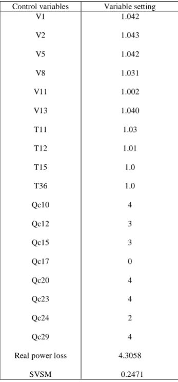
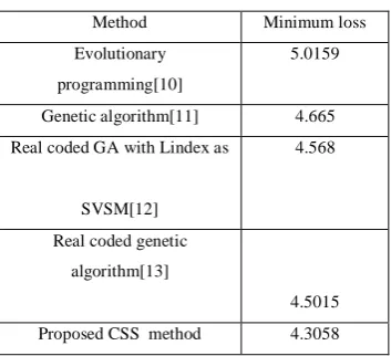
The accuracy of the proposed CSS method is demonstrated by testing it on standard IEEE-30 bus system. The IEEE-30 bus system has 6 generator buses, 24 load buses and 41 transmission lines of which four branches are (6-9), (6-10) , (4-12) and (28-27) - are with the tap setting transformers. The lower voltage magnitude limits at all buses are 0.95 p.u. and the upper limits are 1.1 for all the PV buses and 1.05 p.u. for all the PQ buses and the reference bus. The simulation results have been presented in Tables 1, 2, 3 &4. And in the Table 5 shows the proposed algorithm powerfully reduces the real power losses when compared to other given algorithms. The optimal values of the control variables along with the minimum loss obtained are given in Table 1.
Corresponding to this control variable setting, it was found that there are no limit violations in any of the state variables.
TABLE I. TABLE I.RESULTS OF CSS–ORPD OPTIMAL CONTROL VARIABLES
Control variables Variable setting V1 V2 V5 V8 V11 V13 T11 T12 T15 T36 Qc10 Qc12 Qc15 Qc17 Qc20 Qc23 Qc24 Qc29
Real power loss
SVSM 1.042 1.043 1.042 1.031 1.002 1.040 1.03 1.01 1.0 1.0 4 3 3 0 4 4 2 4 4.3058 0.2471
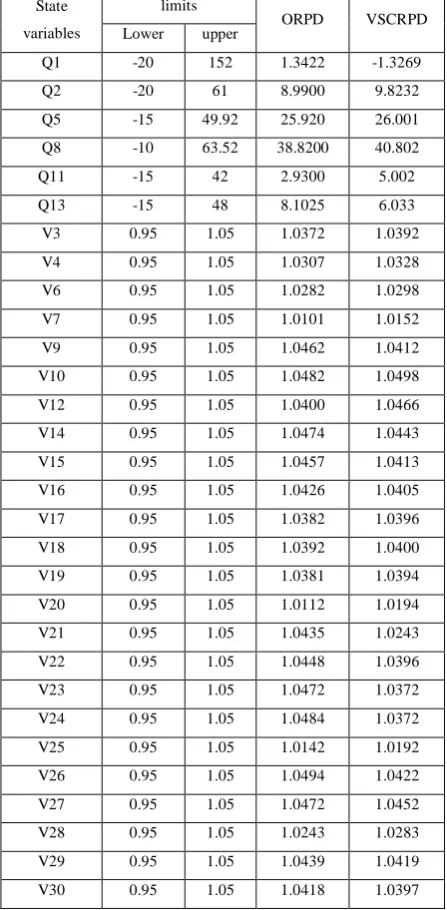
ORPD together with voltage stability constraint problem was handled in this case as a multi-objective optimization problem where both power loss and maximum voltage stability margin of the system were optimized simultaneously. Table 2 indicates the optimal values of these control variables. Also it is found that there are no limit violations of the state variables. It indicates the voltage stability index has increased from 0.2471 to 0.2483, an advance in the system voltage stability. To determine the voltage security of the system, contingency analysis was conducted using the control variable setting obtained in case 1 and case 2. The Eigen values equivalents to the four critical contingencies are given in Table 3. From this result it is observed that the Eigen value has been improved considerably for all contingencies in the second case.
TABLE II. RESULTS OF CSS-VOLTAGE STABILITY CONTROL REACTIVE POWER DISPATCH OPTIMAL CONTROLVARIABLES Control Variables Variable Setting V1 V2 V5 V8 V11 V13 T11 T12 T15 T36 Qc10 Qc12 Qc15 Qc17 Qc20 Qc23 Qc24 Qc29 Real power loss SVSM 1.044 1.043 1.042 1.032 1.006 1.033 0.090 0.090 0.090 0.090 3 4 3 3 0 3 4 4 4.9889 0.2483
TABLE III. VOLTAGE STABILITY UNDER CONTINGENCY STATE
Sl.No Contigency ORPD Setting
VSCRPD Setting 1 28-27 0.1410 0.1432 2 4-12 0.1658 0.1663 3 1-3 0.1774 0.1772 4 2-4 0.2032 0.2043
TABLE IV. LIMIT VIOLATION CHECKING OF STATE VARIABLES
State variables
limits
ORPD VSCRPD Lower upper
Q1 -20 152 1.3422 -1.3269 Q2 -20 61 8.9900 9.8232 Q5 -15 49.92 25.920 26.001 Q8 -10 63.52 38.8200 40.802 Q11 -15 42 2.9300 5.002 Q13 -15 48 8.1025 6.033 V3 0.95 1.05 1.0372 1.0392 V4 0.95 1.05 1.0307 1.0328 V6 0.95 1.05 1.0282 1.0298 V7 0.95 1.05 1.0101 1.0152 V9 0.95 1.05 1.0462 1.0412 V10 0.95 1.05 1.0482 1.0498 V12 0.95 1.05 1.0400 1.0466 V14 0.95 1.05 1.0474 1.0443 V15 0.95 1.05 1.0457 1.0413 V16 0.95 1.05 1.0426 1.0405 V17 0.95 1.05 1.0382 1.0396 V18 0.95 1.05 1.0392 1.0400 V19 0.95 1.05 1.0381 1.0394 V20 0.95 1.05 1.0112 1.0194 V21 0.95 1.05 1.0435 1.0243 V22 0.95 1.05 1.0448 1.0396 V23 0.95 1.05 1.0472 1.0372 V24 0.95 1.05 1.0484 1.0372 V25 0.95 1.05 1.0142 1.0192 V26 0.95 1.05 1.0494 1.0422 V27 0.95 1.05 1.0472 1.0452 V28 0.95 1.05 1.0243 1.0283 V29 0.95 1.05 1.0439 1.0419 V30 0.95 1.05 1.0418 1.0397
TABLE V. COMPARISON OF REAL POWER LOSS
Method Minimum loss Evolutionary
programming[10]
5.0159
Genetic algorithm[11] 4.665 Real coded GA with Lindex as
SVSM[12]
4.568
Real coded genetic algorithm[13]
4.5015 Proposed CSS method 4.3058
6. Conclusion
In this paper a novel approach CSS algorithm used to solve optimal reactive power dispatch problem, considering various generator constraints, has been successfully applied. To handle the mixed variables a flexible representation scheme was proposed. The performance of the proposed algorithm demonstrated through its voltage stability assessment by modal analysis is effective at various instants following system contingencies. Also this method has a good performance for voltage stability Enhancement of large, complex power system networks. The effectiveness of the proposed method is demonstrated on IEEE 30-bus system.
References
[1] O.Alsac,and B. Scott, “Optimal load flow with steady state security”,IEEE Transaction. PAS -1973, pp. 745-751.
[2] Lee K Y ,Paru Y M , Oritz J L –A united approach to optimal real and reactive power dispatch , IEEE Transactions on power Apparatus and systems 1985: PAS-104 : 1147-1153
[3] A.Monticelli , M .V.F Pereira ,and S. Granville , “Security constrained optimal power flow with post contingency corrective rescheduling” , IEEE Transactions on Power Systems :PWRS-2, No. 1, pp.175-182.,1987.
[4] Deeb N ,Shahidehpur S.M ,Linear reactive power optimization in a large power network using the decomposition approach. IEEE Transactions on power system 1990: 5(2) : 428-435
[5] E. Hobson ,’Network consrained reactive power control using linear programming, ‘ IEEE Transactions on power systems PAS -99 (4) ,pp 868=877, 1980
[6] K.Y Lee ,Y.M Park , and J.L Oritz, “Fuel –cost optimization for both real and reactive power dispatches” , IEE Proc; 131C,(3), pp.85-93.
[7] M.K. Mangoli, and K.Y. Lee, “Optimal real and reactive power control using linear programming” , Electr.Power Syst.Res, Vol.26, pp.1-10,1993.
[8] S.R.Paranjothi ,and K.Anburaja, “Optimal power flow using refined genetic algorithm”, Electr.Power Compon.Syst , Vol. 30, 1055-1063,2002.
[9] D. Devaraj, and B. Yeganarayana, “Genetic algorithm based optimal power flow for security enhancement”, IEE proc-Generation.Transmission and. Distribution; 152, 6 November 2005.
[10] Wu Q H, Ma J T. Power system optimal reactive power dispatch using evolutionary programming. IEEE Transactions on power systems 1995; 10(3): 1243-1248
[11] S.Durairaj, D.Devaraj, P.S.Kannan ,’ Genetic algorithm applications to optimal reactive power dispatch with voltage stability enhancement’ , IE(I) Journal-EL Vol 87,September 2006.
[12] D.Devaraj ,’ Improved genetic algorithm for multi – objective reactive power dispatch problem’ European Transactions on electrical power 2007 ; 17: 569-581.
[13] P. Aruna Jeyanthy and Dr. D. Devaraj “Optimal Reactive Power Dispatch for Voltage Stability Enhancement Using Real Coded Genetic Algorithm” International Journal of Computer and Electrical Engineering, Vol. 2, No. 4, August, 2010 1793-8163.
[14]. Kaveh, A., Talatahari, S.: An improved ant colony optimization for constrained engineering design problems. Engineering Computations 27(1) (2010, in press)
[15] Fogel, L.J., Owens, A.J., Walsh, M.J.: Artificial Intelligence Through Simulated Evolution. Wiley, Chichester (1966)
[16] De Jong, K.: Analysis of the behavior of a class of genetic adaptive systems. Ph.D. Thesis, University of Michigan, Ann Arbor, MI (1975)
[17] Koza, J.R.: Genetic programming: a paradigm for genetically breeding populations of computer programs to solve problems.Report No. STAN-CS-90-1314, Stanford University, Stanford, CA (1990)
[18] Holland, J.H.: Adaptation in Natural and Artificial Systems. University of Michigan Press, Ann Arbor (1975)
[19] Goldberg, D.E.: Genetic Algorithms in Search Optimization and Machine Learning. Addison-Wesley, Boston (1989)
[20] Glover, F.: Heuristic for integer programming using surrogate constraints. Decis. Sci. 8(1), 156–166 (1977)
[21] Dorigo, M., Maniezzo, V., Colorni, A.: The ant system: optimization by a colony of cooperating agents. IEEE Trans. Syst.Man Cybern. B 26(1), 29–41 (1996)
[22] Eberhart, R.C., Kennedy, J.: A new optimizer using particle swarm theory. In: Proceedings of the sixth international symposium on micro machine and human science, Nagoya, Japan (1995)
[23] Kirkpatrick, S., Gelatt, C., Vecchi, M.: Optimization by simulated annealing. Science 220(4598), 671–680 (1983)
[24] Erol, O.K., Eksin, I.: New optimization method: Big Bang–Big Crunch. Adv. Eng. Softw. 37, 106–111 (2006)
[25] Kaveh, A., Talatahari, S.: Size optimization of space trusses using Big Bang–Big Crunch algorithm. Comput. Struct. 87(17–18), 1129–1140 (2009)
[26] Rashedi, E., Nezamabadi-pour, H., Saryazdi, S.: GSA: a gravitational search algorithm. Inf. Sci. 179, 2232– 2248 (2009)
[27] Halliday, D., Resnick, R., Walker, J.: Fundamentals of Physics, 8th edn. Wiley, New York (2008)
[28] Kaveh, A., Talatahari, S.: Particle swarm optimizer, ant colony strategy and harmony search scheme hybridized for optimization of truss structures. Comput. Struct. 87(5–6), 267–283 (2009)
[29] Coello, C.A.C.: Theoretical and numerical constraint-handling techniques used with evolutionary algorithms: a survey of the state of the art. Comput. Methods Appl. Mech. Eng. 191(11–12), 1245–1287 (2002)
[30] Kaveh, A., Talatahari, S.: A particle swarm ant colony optimization for truss structures with discrete variables. J. Constr.Steel Res. 65(8–9), 1558–1568 (2009)
K. Lenin has received his B.E., Degree, electrical and electronics engineering in 1999 from university
of madras, Chennai, India and M.E., Degree in power systems in 2000 from Annamalai University,
TamilNadu, India. Now pursuing Ph.D., degree at JNTU, Hyderabad,India.
Bhumanapally. RavindhranathReddy, Born on 3rd September,1969. Got his B.Tech in Electrical &
Electronics Engineering from the J.N.T.U. College of Engg., Anantapur in the year 1991. Completed his M.Tech in Energy
Systems in IPGSR of J.N.T.University Hyderabad in the year 1997. Obtained his doctoral degree from JNTUA,Anantapur
University in the field of Electrical Power Systems. Published 12 Research Papers and presently guiding 6 Ph.D. Scholars.
He was specialized in Power Systems, High Voltage Engineering and Control Systems. His research interests include
Simulation studies on Transients of different power system equipment.
M. Surya Kalavathi has received her B.Tech. Electrical and Electronics Engineering from SVU, Andhra
Pradesh, India and M.Tech, power system operation and control from SVU, Andhra Pradesh, India. she
received her Phd. Degree from JNTU, hyderabad and Post doc. From CMU – USA. Currently she is
Professor and Head of the electrical and electronics engineering department in JNTU, Hyderabad, India
and she has Published 16 Research Papers and presently guiding 5 Ph.D. Scholars. She has specialised
in Power Systems, High Voltage Engineering and Control Systems. Her research interests include
Simulation studies on Transients of different power system equipment. She has 18 years of experience. She has invited for
various lectures in institutes.