©2012 JNAS Journal-2012-1-1/30-34 ISSN 0000-0000 ©2012 JNAS
An Application of Bayes Regression for a Small Sample
N. Abbasi* , M. Shokrizadah
Department of Statistics, Payame Noor University, I. R. Iran
Corresponding author Email : [email protected]
ABSTRACT: Main purpose of this article is to have a posterior distribution of the model structural parameters in the regression model with elliptical measurement error based on prior distribution and considering the previous one was gained multivariable β it is not easy to produce data from it to measure the previous distribution mean. So we use Gibbs sampling method stated by Arellano and Bolfarine(1998). Finally we stated an application of the regression model.
Keywords: Elliptical distribution, Regression model with measurement error, Byes estimation, Gibbs algorithm
INTRODUCTION
In this article we examine one variable regression of response ‘y’ on the random variable ξ under observations
of *( ) ( )+ which ( ) measures the quantity ( ) with the measurement error.
Now we suppose that *( ) ( )+ observations come from a model with a measurement error shown by following equations :
where ( ), ( ) , ( ) and is component of a vector as ( ) . Having supposed that the measurement errors have been distributed normally Lindley & El-Sayyad (1968) examined the model. Also the state was discussed by many scientists. You may refer to Kendal and Stuart (1961), Johnston(1963) and Mandansky(1959) for more details. The essential supposition is that the measurement errors have elliptical distribution. Hereafter ( ) is symbol of n-variable elliptical distribution with mean and
dispersion matrix , and density materials function ( ), if and only if its probable density is:
( | ) | | ( )( ( ))
where ( ) ( )| | ( ) and ( ) should be nonnegative function and be right in the condition:
∫ ( )( ) . /
Now, we suppose that the regression model errors have following conditional distribution:
( )| ( ( ) )
Having supposed that ( ) has squared radial distribution Vidal and Arellano-Valle did the Bayes inference on the model (1) and (2). Now suppose following the elliptical model :
| ,( )
( | )
( | )
( )
( )
31
where h is generating function and and are clear and ( | ) is the conditional generating function of the next 2n and previous distribution is a squared radial function with ‘d’ freedom degree. By virtue of the model (5)-(3) Vidal & Arellano-Valle proved that the posterior distribution ( ) is as follows:
( | ) ( ‖ ‖ ‖ ‖ ) ( | )
where ( ) and , - .By integrating on parameter it is possible to have marginal distribution as
follows :
( | ) . ( )‖ ‖ /
( ) (6)
Posterior Average of Structural Parameters
In this section supposing is unknown and the usual a priori distribution the Bayes model has been given in (3)-(5):
( )
Now we should find complete conditional algorithm for Gibbs algorithm and estimate a priori average estimation β. Supposing the non-information posterior distribution ( ) for α we have:
( | ) (
‖ ‖ )
which is the gamma – gamma distribution kernel with following parameters:
[ ⁄ ( ) ‖ ‖ ].
If ( ) ( ) , ( | ) is appropriate distribution. Now considering the β is multivariable it is
uneasy to produce data from it to be able to estimate the posterior distribution average . So we use Gibbs sampling method. Algorithm is a device to produce random data from multivariable distribution from which it is uneasy to produce data. Here we may use Gibbs algorithm in detail. We put ̂ for and produce two following steps::
( | )
( | )
This algorithm is stated in Vidal and Bolfarine (2011). In next section we examine the findings on real data.
Examining scientific production data
In this section we examine the findings on real data. Here we use the model defined in (1) . The data in following Table show two variables: Nos. of the articles and score of participation in M.A. (M.S.) thesis. The data are about 17 members of scientific board in one centre of Payame Noor University in 2011. The members scientific productions depend on several factors , but their professional and internal motives to do and create science vary . It should be emphasized that if such activities are always protected, related participation and scientific productions increase, too. So we consider financial factors with participation variable in M.A. (M.S.) theses like X and relation in the (1) relations we may have a more exact model for and Y.
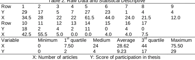
Table 2. Raw Data and Statistical Descriptive
Row 1 2 3 4 5 6 7 8 9
Y 29 17 5 7 27 23 1 4 4
X 34.5 28 22 22 61.5 44.0 24.0 21.5 12.0
Row 10 11 12 13 14 15 16 17
Y 18 2 4 2 11 0 4 0
X 42.5 55.5 5.0 0.0 0.0 4.0 4.0 7.5
Variable Minimum 1st quartile Medium Average 3rd quartile Maximum
X 0 7.50 24 28.62 44 75.50
Y 0 2 4 9.23 17 29
X: Number of articles Y: Score of participation in thesis
32
Figure 1. Scientific Productions Rate
As you see in Figure (6-4) two maximum likelihood estimation fitting lines and total least errors squares are intersected; it might be seen in previous example, too .In Table (5-4) it may be seen the estimations by three mentioned methods. In third column of the Table (5-4) low error square average MSE indicates the model gained by PME with a very little difference from the Model LSE is better than two other models.
Table 4. The rates estimated by regression parameters
Β0 Β1 MSE
MLE 3.43951 0.20458 321.1932
LSE 4.25631 0.17603 296.1852
PME 4.27037 0.17367 176.0832
As it is clear from Table (4) the Bayes estimation rate is near the total least errors squares described analytically in section (3-4).
Table 5. Regression Parameters Summary :
Average Medium Standard deviation
Metropolis- Within-Gibbs ΒΒ0 4.27037 4.23148 0.01468
1 0.17367 0.17459 0.00052
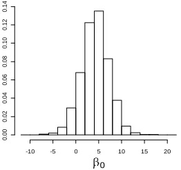
We drew the Β0 posterior distribution histogram by software ‘F’ and showed that it has symmetric distribution .
Figure 2. Β0 posterior distribution histogram
Figure (2–4): We drew Β1 posterior distribution histogram; here it may be seen the symmetry.
0 5 10 15 20 25 30 35
0
5
10
15
20
25
30
35
x
y
PME LSE MLE
0
-10 -5 0 5 10 15 20
0
.0
0
0
.0
2
0
.0
4
0
.0
6
0
.0
8
0
.1
0
0
.1
2
0
.1
33
Figure 3: Β1 posterior distribution histogram
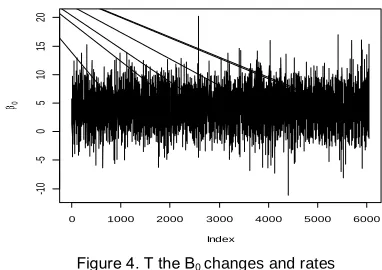
Figure (4) shows the Β0 changes and rates. Here it may be seen the Β0 distribution symmetry, too.
Figure 4. T the Β0 changes and rates
Figure (5) shows the Β1 changes and rates. Here it may be seen the Β1 distribution symmetry, too.
Figure 5. The Β1 changes and rates
Findings
The main purpose is to find a regression model by two visible variables with an average in which no common relation with third variable is visible. In recent applied subject it was shown that the regression model gained by posterior data distribution may be a linear model with the least error squares method. If there are more comprehensive and better knowledge about the variables Β1 and Β1 behavior and the posterior distribution is more proper, the findings are more exact.
1
-0.4 -0.2 0.0 0.2 0.4 0.6
0
1
2
3
0 1000 2000 3000 4000 5000 6000
-1
0
-5
0
5
10
15
20
Index
0
0 1000 2000 3000 4000
-0
.2
0.
0
0.
2
0.
4
0.
6
Index
34
REFERENCES
Bernardo, J.M., Smith, A.F.M., 1994, Bayesian Theory. Wiley, Chichester.
Bolfarine, H., Arellano-Valle, R.B., 1998. Weak non differential measurement error models. Statistics & Probability Letters 40, 279–287.
Bolfarine, H., Arellano-Valle, R.B., 2005. Elliptical measurement error models—a Bayesian approach. In: Dey, D.K., Rao, C.R. (Eds.), Bayesian Thinking:
Modeling and Computation. In: Handbook of Statistics, vol. 25. Elsevier B.V., North-Holland, pp. 669–688.
Carrol, R.J., Ruppert, D., Stefanski, L.A., Crainiceanu, C.M., 2006. Measurement Error in Nonlinear Models: A Modern Perspective. Chapman & Hall, CRC, Boca Raton.
Chen, M.H., Shao, Q.M., 1999. Monte Carlo estimation of Bayesian credible and HPD intervals. Journal of Computational and Graphical Statistics 8, 69–92.
Cheng, C.-L., van Ness, J.W., 1999. Statistical Regression with Measurement Error. In: Kendall’s Library of Statistics, vol. 6. Arnold, London.
Fang, K.T., Kotz, S., Ng, K.W., 1990. Symmetric Multivariate and Related Distributions. Chapman & Hall, London, New York. Fuller, W.A., 1987. Measurement Error Models, vol. 1. John Wiley & Sons, New York.
Hobert, J.P., Robert, C.P., Goutis, C., 1997. Connectedness conditions for the convergence of the Gibbs sampler. Statistics & Probability Letters 33, 235–240.
Kelly, G.E., 1984. The influence function in the errors in variables problem. The Annals of Statistics 12, 87–100.
Lindley, D.V., El-Sayyad, G.M., 1968. The Bayesian estimation of a linear functional relationship. Journal of the Royal Statistical Society. Series B 30, 190–202.
O’Hagan, A., 1994. Bayesian Inference. In: Kendall’s Advanced Theory of Statistics, vol. 2B. Edward Arnold, London. Robert, C.P., Casella, G., 2004. Monte Carlo Statistical Methods, second ed. Springer, New York.
Vidal, I., Arellano-Valle, R. B., 2010. Bayesian inference for dependent elliptical measurement error models. Journal of Multivariate Analysis 101, 2587–2597.