AN ALGORITHM FOR PHOTOVOLTAIC SYSTEM UNDER PARTIAL SHADING CONDITIONS AND LOAD VARIATION

AN ALGORITHM FOR PHOTOVOLTAIC SYSTEM

UNDER PARTIAL SHADING CONDITIONS AND

LOAD VARIATION

R.Ramya

, Dr.C.Kumar

1

PG Scholar,2Associate ProfessorDepartment of EEE,

Bannari Amman Institute of Technology, Sathyamangalm, TamilNadu(India)

ABSTRACT

Under partial shading situations, multiple peaks are observed in the power–voltage (P V) characteristics

curve of a photovoltaic (PV) array, and the conventional maximum power point tracking (MPPT) algorithms

may fail to track the global maximum power point (GMPP). Therefore, this paper proposes an enhanced

incremental conductance (Inc Cond) algorithm that is able to track the GMPP in partial shading conditions

and load variation. A novel algorithm is used to control the duty cycle of the dc–dc converter in order to make

sure fast MPPT process. Simulation works are carried out to calculate the effectiveness of the proposed

algorithm under partial shading condition and load variation. The results show that the proposed novel

algorithm is able to track the GMPP exactly in different types of partial shading conditions, and the response

while ch a n g i n g load c o n d i t i o n and solar irradiation are faster than the conventional Incremental

Conductance algorithm. Hence, the efficiency of the proposed novel algorithm under partial shading condition

and load variation is validated in this paper.

Keywords: DC–DC Converter, Maximum Power Point Tracking (MPPT), Partial Shading

Condition, Load Variation, Photovoltaic (PV) System.

I. INTRODUCTION

Solar is the Latin word for sun a powerful source of energy that can be used as heat, cool and light our home and business etc. That’s because more energy from the sun falls on the earth that is used by everyone in the world. The technology is used to convert the sunlight in to usable energy for our application such as solar thermal and solar photovoltaic (PV). The PV is used to convert the solar energy in to electricity. Maximum power point tracker is used track the maximum available solar energy efficiently from the PV panel. Maximum power point tracking algorithm that include in charge controller used for extracting available maximum power from the PV module under certain conditions. The voltage at which PV module can produce maximum power is called maximum power point.

models of digital MPPT controller available with Micro processor controller. They know when to adjust the output that is being select to the battery and actually shut down for few micro second and look at the solar panel and battery any needed adjustment[5].

Now a days for increase in solar power generation many algorithm are used in MPPT to track the maximum power from the solar panel. The algorithms are Incremental conductance, fuzzy logic perturbation and observer, neutral network, partial swarm [6]-[8]. These algorithms are not efficient to track the maximum available power from the PV panel under partial shading condition and load variation [9]. These have been efficiently tack the maximum available power under uniform irradiation condition having only one maximum power point exists in the power –voltage (PV) curve. But in partial shading condition having multiple MPPs in the power- voltage curve. [11][12] These types of algorithm are not efficient to track the GMPP among the local maximum power point (LMPP).

The Perturbation and Observer algorithm took long time to track the Global Maximum Power Point (GMPP) under partial shading condition [13]. Focusing on multiple peaks during partial shading condition few solutions have been proposed by altering the conventional algorithm [14]-[16]. The Incremental Conductance algorithm is modified to track the GMPP but it required additional measurements so the hardware goes to complex. The perturbation and observation algorithm is proposed for tuning the highest and lowest to identify all possible MPPs [16]. The peak can be successfully identified but the Perturbation and Observer algorithm takes long time to track the global maximum power point (GMPP) under partial loading condition [17].

The Hill climbing algorithm based on fuzzy logic is introduced to track GMPP, in this algorithm all the MPP values are stored in microcontroller and algorithm is later implemented to track GMPP based on the record. In these type of algorithm having long processing time in perturbing and storing all possible MPPs, the use of fuzzy logic also involves complicated fuzzification and defuzzification [18][19]. A comparative study on voltage curve (P-V) under partial shading condition was reported, it shows that the peaks in power-voltage curve occurred approximately at the multiples of 80% open circuit power-voltage. The magnitude of P-V curve peaks show the increasing before the GMPP and decreasing after the GMPP [20].Based on that the P&O algorithm failed to track the GMPP effectively under partial shading condition. In this paper Modified Incremental Conductance algorithm has been introduced to track the GMPP effectively under Partial Shading Condition and Load Variation [21].

Fig.1. Proposed PV system with MPPT controller

II. PV ARRAY UNDER PARTIAL SHADING CONDITION

The PV cells are connected electrically in series or parallel circuits to produce higher voltage, current and power levels. The PV module consists of PV cell circuits sealed in an environmentally protective laminate, and are the fundamental building blocks of PV system. A PV array is the complete power generating unit, consisting of many number of PV modules in series and parallel. When any one of the PV module does not produce the power due to shaded effect or does not attain solar irradiation it effect the power generated by other PV modules. Because the power generated from the PV array is the arrangement of the power consequent from each module. The array operates at current (IA), the shaded portion mandatory to operate at reverse biased condition and turn as a load instead of power source.

Fig.2. PV array under partial shading condition

III. PROPOSED ALGORITHM

In the proposed algorithm, the perturbation and observation algorithm can be replaced by modified Incremental conductance algorithm .The modified Inc conductance algorithm having the ability to track MPP under fast varying weather condition. It takes less time to track MPP at LMPP to GMPP. IN addition a novel is introduced to very fast tracking of MPP under multiple peaks. The critical statement point referred are the occurrences of peak voltage at multiples of 0.8*Voc and consecutive increasing and decreasing of peaks magnitude. The magnitude of the peak is increasing up to the GMPP and decreasing during PV crossed either side. There are three multiple peaks of P-V curve shown in Fig.3.

Fig.3. P-V curves of the PV array under partial condition. (a) GMPP located at the middle of P-V curve. (b) GMPP located at the left end of P-V curve.

(c) GMPP located at the right of P-V curve.

The GMPP peak located in three ways, first the GMPP is located in the central of three consecutive peaks, and it has the peak magnitude or in another case the GMPP is to be found in th e P-V curve at both right and left end. Therefore, there are only three possible types of multiple peaks P –V curve, as shown in Fig. 3 (a). The first type is where the GMPP is in a mid of the others MPPs, as in Fig.3 (b). The other two options are the location of the GMPP at the left peak and right peak side of the P-V curve and the magnitude is decreasing as the peaks are additional left from the GMPP, as shown in Fig. 3 (c).

Among all the MPPs, the proposed algorithm finds three successive peaks and finds the one which has the highest magnitude. If the GMPP is not in the central of the three peaks, the algorithm continues to search until the GMPP is in the middle or until the end of the P –V curve where the minimum or maximum possible voltage is reached. The algorithm used to track the GMPP in three different types of multiple peaks P-V curve is explained in the following section. The two variables required in the algorithm are the open-circuit voltage of the PV module Vco and the series-connected maximum number of module Nmax.

Case 1-GMPP Located in Between the Other MPPs:

at point A by using conventional Inc Cond algorithm is in Fig. 3 (a). When the first MPP is tracked, the duty cycle of the converter and the power of the MPP are stored into Duty1 and Pmpp1 (block 4).The Vmax is the multiplication of Vco and Nmax , has not been attained yet in th e (block 6), the algorithm will proceed to the right of point A to search for the next MPP. As stated in [22], the Voltage of MPPs are 0.8*Voc from each other and by adding 0.8*Voc Vmpp1 the reference voltage is increased (block 6). In (block 8) MPPT tracking subroutine shown in Fig. 5 is used to ensure that the operating point of the PV array is touched near point B in Fig. 3(a) before (block9) the conventional Incremental Conductance algorithm is used to track the MPP at point B.

Then, (block 10) the duty cycle of the converter and the power of the MPP at point B are stored as Duty2 and Pmpp2.If point B is greater than point A that is Pmpp2 is greater than Pmpp1 (block 11), as shown in Fig. 3(a), then the algorithm goes to (block 12) and Pm p p 1 _and Duty1 (point A) are stored into Pmpp3 and Duty3. Then the

(point B) Pmpp2 and Duty2 are stored into Pmpp1 and Duty1 .The Pmpp1 permanently contains the data of the MPP, which has the highest magnitude now, the algorithm returns to (block 6). If the maximum voltage has not been attained yet, the algorithm will continue to catch Pmpp2at the right of pmpp1 (blocks 7–10). At point C the

algorithm found that Pmpp2 is less than Pmpp1 (point B), the algorithm goes to (bl ock 13). Since Pmpp3

contained the data of point A, the algorithm uses the duty cycle as Duty1 of the converter (block 14) after that

goes to (block 22).

)

1

..(

...

...

...

06

.

0





v

I

dv

dI

Then, (1) is used to ensure operating that the point of the PV system remains at the GMPP. Usually, the right side of (1) is defined as zero. Due to truncation error practically, it is difficult to obtain the zero value [35]. Therefore, to increase the efficiency of a PV system the permitted error of 0.06 is used to stop the oscillation during steady state condition .This value is selected based on the converter duty cycle step size (0.005), and with this acceptable error, the acceptance on the MPPs of PV array is nearby 0.7%. Then, the algorithm keeps looping until there is a variation on solar irradiation or load in (blocks 22, 23) [i.e., (1) no longer satisfied]. Subsequently, the algorithm goes into (block 24) to regulate the direction of variation in the voltage and current of the PV array. The changes in the voltage and current of the PV array during change in load or solar irradiation are noted. When the different directions of variation in voltage and current, there must be a variation in the load resistance. Therefore calls the load variation subroutine shown in Fig. 4 to guarantee that the PV array returns to the GMPP quickly. If there is a change in directions of voltage and current is the same variation in solar irradiation. Then, the algorithm starts to search from (b l o c k 3) again to track for the new GMPP.

Measure Vpv & Ipv

Using Vpv & Ipv to find Rload

Using Vmpp1,Impp1,Rload to find the duty cycle

Incremental conductance algorithm

return

Measure Vpv & Ipv

Using Vpv & Ipv to find Rload

Using Vmpp1,Impp1,Rload to find the duty cycle

dI<0.03

return Yes

Fig.4.Subroutine flowchart for Load Variation Fig.5.Subroutine flowchart for MPPT

Initialize Pmpp1=Pmpp2=Pmpp3=0 Set Vmax=Nmax*Voc Vmin=0 Call Incremental conductance Store Pmpp1,Duty1 Vmax<Vcal Vcal=Vmpp1+0.8*Vin Vref=Vmpp1+Voc Call MPPT subroutine

Call inc conductance

Store Pmpp2,Duty2 Pmpp<=Pmpp1 Pmpp3=Pmpp1 Duty3=Duty1 Pmpp1=Pmpp2 Duty1=Duty2 Pmpp3>0 Duty cycle=Duty1 Vmpp1-0.8*Voc<Vmin Vref=Vmpp1-Voc

Call MPPT subroutine

Call incremental conductance

Store Pmpp3 duty 3

Pmpp3<=Pmpp1 Pmpp2=Pmpp1 Duty2=Duty1 Pmpp1=Pmpp3 Duty1=Duty3 Mod of Gd+Gs<0.06 dI>0&&dV<0 Or dI<0&&dV>0 Call load variation

subroutine No change 1 2 3 4 5 6 7 8 9 10 11 12 13 14 15 16 17 18 19 20 21 22 23 24 25 yes No yes No yes No No yes NO yes yes yes No No

Fig.6.Flowchart of the proposed algorithm Case 2-GMPP found at the Left Side of All the MPPs:

any value yet (block 14) and the minimum voltage value V_{min, which is equal to zero has not been} achieved yet (block 15) at (point F) the algorithm will continue to find P_mpp3 at the left of P_mpp1.

In the reference voltage is reduced by 0.8∗Vco (block 16) and MPP tracking subroutine (block 17) is called to converge the operating point of the PV array close to the MPP at point F shown in Fig.3(b) before the conventional Incremental Conductance algorithm (block 18) is used to track the MPP at point F. The maximum power and duty cycle of point F are stored into Pmpp3 and Duty3 (block 19). Since (point F) is greater than

(point D) that is Pmpp3 is greater than Pmpp1, the data of point D are now stored into P_mpp2 and Duty2 and the data of point F are now stored into P_{mpp1 and} D_{uty1 (block 21). After that, the algorithm goes back to (block} 15), and D_{uty1 is used as the duty cycle of the converter because of minimum voltage} V_{min is attained. In} this case, the PV system operates at the left peak side of the P–V curve (point F) is the GMPP. Finally, the algorithm is looping between blocks (22–23), observing any deviation in solar irradiation and load.

Case 3-GMPP located at the Right Side of All the MPPs:

Initially, all the parameters are set to zero (blocks 1 and 2). Then, this new algorithm conventional Inc Cond (block 3) is used to track the initial MPP at point G in Fig. 3(c). After that Pmpp1 and Duty1 (block 4), data of point G are stored into the algorithm goes to the right side of Pmpp1 to track Pmpp2 (blocks 7–10) at point H since the maximum voltage Vmax (block 6) has not been attained yet. Since Pmpp2 is greater than Pmpp1, the algorithm back to (block 12) and the data of point G (Pmpp1) are kept in P_mpp3.Temporarily; the data of point H Pmpp2 are stored into Pmpp1. Then, the algorithm stay to find the MPP, point I (blocks 7– 10) at the right of Pmpp1 (point H) since Vmax has not been touched yet (block 6). Then, the algorithm goes to (block 12) again; later the MPP at point I P_mpp2 is greater than point H P_mpp1. Hence, the data of point H are stored into P_mpp3, and the data of point I are stored into P_mpp1. After this, the algorithm observes that maximum voltage Vmax has extended (block 6) and Pmpp3 (point H) previously has a value (block 13). Hence, (block 14) Duty1 is used as the duty cycle of the converter to ensure that the PV array controls at the GMPP, point I. Finally, the algorithm keeps searching at (blocks 22 and 23) and observes for any changes in load or solar irradiation.

IV. DUTY CYCLE CONSUMPTION

duty cycle, the MOSFET operate at high frequency compared to IGBT and having low cost. Hence, MOSFET can be used to DC-DC converter to obtain desired output.

)

2

...(

...

...

1

V

D

D

V





)

3

...(

...

...

1

I

D

D

I





From (2) & (3) to obtain

)

4

...(

...

...

)

1

(

Z

D

D

Z





Where D is the duty cycle of the dc–dc converter; Input voltage of the D C- DC converter is Vin or the voltage of the PV array is Viv; th e input current of the DC -DC converter is Ian or the current of the PV array I_vy; Zin is the input impedance of the converter or the impedance realized by the PV array; and Zout is the output impedance of the converter or is the load impedance Zload.

In the PV system, (4) can be rewritten to obtain (5) and (6)

)

5

.(

...

...

)

1

(

Z

D

D

I

V





)

6

.(

...

...

)

1

(

I

V

D

D

Z





When the duty cycle D is known, the load impedance Zload of the output converter can be calculated by using voltage of PV array (Vpv) and the current of the PV array (Ivy) under any operating point by using (6). After obtained the load impedance, (6) can be altered into (7). With the required voltage and current of the PV array, the duty cycle can be find by using (8). When this duty cycle is applied on the converter, to operate at the desired voltage and current the PV system can be modulated.

)

7

.(

...

...

)

1

(

Z

I

V

D

D





Where a= (Ivy/Viv) Load

In this novel, by using equation (6) the load of the PV system is calculated. Then, using equation 8) to obtain the duty cycle of the converter the desired value of voltage and current are substituted. Hence, the duty cycle can be obtained and modulated quickly to obtain the desired output power.

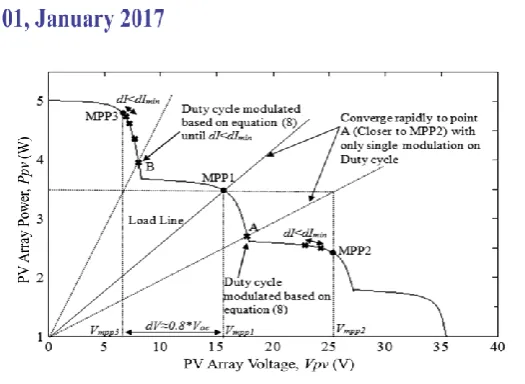
As shown in Fig. 7, when MPP1 is conventional Inc Cond algorithm can be used to track MPP1 the proposed algorithm goes to the right of MPP1 to examine for other MPPs. As aforementioned, the voltages of MPPs are almost 0.8∗ V_{co. Left from each other By adding 0}.8∗ V_{co in to} V_mpp1 to get the voltage of MPP2 V_{mpp2. Then,} to obtain the duty cycle by using (8) the current of MPP2 is

Fig.7. I –V curve of PV array under partial shading conditions.

also required, but the current at MPP2 is unknown. Therefore, the current at MPP1 and the voltage at Vmpp2 are substituted into (8), and the operating point of the PV array is converged to point A rapidly. After this, to get the next duty cycle the current at point A and Vmpp2 are substituted again into (8). This process repeat until to obtain a point where the difference in current d id is slighter than a minimum value d Imin. Then, the conventional Inc. Cond algorithm is used to track the MPP2. When the operating point is near to MPP2 only this condition the conventional Inc Cond algorithm can be used or else the same MPP (MPP1) will be tracked. Therefore, d Imin is set to be 0.03 in this proposed system based on try and error observation from the simulation. The same technique is used in the searching of MPP3 at the left of MPP1. Current at MPP1 and

Vmpp3 ( obtained by deducting 0.8∗ Vco. from Vmpp1) are substituted into (8) to obtain the duty cycle. Then,

the operating point of the PV array is converged to point B rapidly. This procedure continues until d id is smaller than d Imin and then the proposed algorithm is used to track MPP3. Showing the simulation results of the proposed algorithms. The proposed algorithm is able to expanse the preferred voltage at t = 0.6 s, but the conventional algorithm required 1.6 s. With the fast modification in the voltage of the PV array, the MPPs can be attained rapidly.

V. SIMULINK MODELING

Fig 8 shows that Simulink design for solar module. The solar cells 36 are connected in series, the required modeling parameters are Isc=4.7 A, Io=9.2119E-10A, Kb=1.138E-23J/k, q=1.6E-19c,Rs=0.1293 Ω, Rsh=12.463 Ω, α=3.8E-3, Tref=298K, Eg=1.12 ev. Fig 9 shows that PV panel with bypass diode under the irradiance values are 0.6W/m2, 0.4 kW/m2, 1.0 kW/m2, 0.7 kW/m2 . Fig. 10 shows that incremental conductance Simulink design.

Fig.8.Simulink modeling of solar module

Fig.10. Shows that simulink mosel of incremental conductance algorithm.

VI. RESULTS AND DISCUSSION

Fig.11. shows that design for proposed method fig.12. shows that mosfet gate pulse

Fig.13. shows that output waveform of proposed system for load(R=10)

VII. CONCLUSION

In this paper, the global maximum power point for PV array can be tracked under partial shading and load variation condition. This algorithm is used to modulate the duty cycle of the DC-DC converter and thus , the tracking speed of the MPPT controller is improved.The simulation showed that the proposed algorithm is able to track the GMPP accurately and thus reduces the power losses faced by the conventional algorithm. As a conclusion, a novel modified incremental conductance algorithm performed better in tracking the GMPP under partial shading and load variation, as compared to conventional incremental conductance algorithm.

REFERENCES

[1] S. Mekhilef, R. Saidur, and A. Safari, “A review on solar energy use in industries,” Renew. Sustain. Energy Rev., vol. 15, no. 4, pp. 1777–1790, May 2011.

[2] S. Mekhilef, A. Safari, W. E. S. Mustaffa, R. Saidur, R. Omar, and M. A. A. Younis, “Solar Energy in Malaysia: Current state and prospects,” Renew. Sustain. Energy Rev., vol. 16, no. 1, pp. 386-396, Jan. 2012.

[3] K. H. Solangi, M. R. Islam, R. Saidur, N. A. Rahim, and H. Fayaz, “A review on global solar energy policy,” Renew. Sustain. Energy Rev., vol. 15, no. 4, pp. 2149–2163, May 2011.

[4] T. Esram and P. L. Chapman, “Comparison of photovoltaic array maximum power point tracking techniques”,IEEE Trans. Energy Convers., vol. 22, no. 2, pp. 439–449, Jun. 2007.

[5] M. A. G. de Brito, L. Galotto, L. P. Sampaio, G. de Azevedo e Melo, and C. A. Canesin, “Evaluation of the main MPPT techniques for photovoltaic applications,” IEEE Trans. Ind. Electron., vol. 60, no. 3, pp. 1156–1167, Mar. 2013.

[6] B. N. Alajmi, K. H. Ahmed, S. J. Finney, and B. W. Williams, “Fuzzy-logic-control approach of a modified hill-climbing method for maximum power point in microgrid standalone photovoltaic system,” IEEE Trans. Power Electron., vol. 26, no. 4, pp. 1022–1030, Apr. 2011.

[7] A. K. Abdelsalam, A. M. Massoud, S. Ahmed, and P. N. Enjeti, “High-performance adaptive perturb and observe MPPT technique for photovoltaic-based microgrids,” IEEE Trans. Power Electron., vol. 26, no. 4, pp. 1010–1021, Apr. 2011.

[8] P. E. Kakosimos, A. G. Kladas, and S. N. Manias, “Fast photovoltaic- system voltage- or current-oriented MPPT employing a predictive digital current-controlled converter,” IEEE Trans. Ind. Electron., vol. 60, no. 12, pp. 5673–5685, Dec. 2013.

[9] O. Lopez-Lapena, M. T. Penella, and M. Gasulla, “A closed-loop maxi- mum power point tracker for subwatt photovoltaic panels,” IEEE Trans. Ind. Electron., vol. 59, no. 3, pp. 1588–1596, Mar. 2012. [10] N. Femia, G. Petrone, G. Spagnuolo, and M. Vitelli, “Optimization of perturb and observe maximum

power point tracking method,” IEEE Trans. Power Electron., vol. 20, no. 4, pp. 963–973, Jul. 2005. [11] L. Whei-Min, H. Chih-Ming, and C. Chiung-Hsing, “Neural-network- based MPPT control of a

Dec. 2011.

[12] T. Shimizu, O. Hashimoto, and G. Kimura, “A novel high-performance utility-interactive Photovoltaic inverter system,” IEEE Trans. Power Electron., vol. 18, no. 2, pp. 704–711, Mar. 2003.

[13] P. S. Shenoy, K. A. Kim, B. B. Johnson, and P. T. Krein, “Differential power processing for increased energy production and reliability of pho- tovoltaic systems,” IEEE Trans. Power Electron., vol. 28, no. 6, pp. 2968–2979, Jun. 2013.

[14] R. Alonso, P. Ibaez, V. Martinez, E. Roman, and A. Sanz, “An innovative perturb, observe and check algorithm for partially shaded PV systems,” in Proc. 13th Eur. Conf. Power Electron. Appl., 2009, pp. 1–8. [15] J. Young-Hyok, J. Doo-Yong, K. Jun-Gu, K. Jae-Hyung, L. Tae-Won, and W. Chung-Yuen, “A real

maximum power point tracking method for mismatching compensation in PV array under partially shaded conditions,” IEEE Trans. Power Electron., vol. 26, no. 4, pp. 1001–1009, Apr. 2011.

[16] E. Koutroulis and F. Blaabjerg, “A new technique for tracking the global maximum power point of PV arrays operating under partial-shading conditions,” IEEE J. Photovolt., vol. 2, no. 2, pp. 184–190, Apr. 2012.

[17] N. Tat Luat and L. Kay-Soon, “A global maximum power point tracking scheme employing Direct search algorithm for photovoltaic systems,” IEEE Trans. Ind. Electron. vol. 57, no. 10, pp. 3456– 3467, Oct. 2010.

[18] B. N. Alajmi, K. H. Ahmed, S. J. Finney, and B. W. Williams, “A maximum power point tracking technique for partially shaded photovoltaic systems in microgrids,” IEEE Trans. Ind. Electron., vol. 60, no. 4, pp. 1596-1606, Apr. 2013.

[19] M. Miyatake, M. Veerachary, F. Toriumi, N. Fujii, and H. Ko, “Maxi- mum power point tracking of multiple photovoltaic arrays: A PSO approach,” IEEE Trans. Aerosp. Electron. Syst., vol. 47, no. 1, pp. 367–380, Jan. 2011.

[20] K. Ishaque and Z. Salam, “A deterministic particle swarm optimization maximum power point tracker for photovoltaic system under partial shading condition,” IEEE Trans. Ind. Electron., vol. 60, no. 8, pp. 3195– 3206, Aug. 2013.

[21] K. Ishaque, Z. Salam, M. Amjad, and S. Mekhilef, “An improved particle swarm optimization (PSO)-based MPPT for PV with reduced steady-state oscillation,” IEEE Trans. Power Electron., vol. 27, no. 8, pp. 3627–3638, Aug. 2012.

[22] H. Patel and V. Agarwal, “Maximum power point tracking scheme for PV systems operating under partially shaded conditions,” IEEE Trans. Ind. Electron., vol. 55, no. 4, pp. 1689–1698, Apr. 2008.

[23] A. Zbeeb, V. Devabhaktuni, and A. Sebak, “Improved photovoltaic MPPT algorithm adapted for unstable atmospheric conditions and partial shading,” in Proc. Int. Conf. Clean Elect. Power, 2009, pp. 320–323. [24] Y. A. Mahmoud, X. Weidong, and H. H. Zeineldin, “A parameterization approach for enhancing PV

model accuracy,” IEEE Trans. Ind. Electron., vol. 60, no. 12, pp. 5708–5716, Dec. 2013.

[25] C. Olalla, D. Clement, M. Rodriguez, and D. Maksimovic, “Architectures and control of submodule integrated DC–DC converters for photovoltaic applications,” IEEE Trans. Power Electron., vol. 28, no. 6, pp. 2980–2997, Jun. 2013.

2957–2967, Jun. 2013.

[27] S. Poshtkouhi, V. Palaniappan, M. Fard, and O. Trescases, “A general approach for quantifying the benefit of distributed power electronics for fine grained MPPT in photovoltaic applications using 3-D modeling,” IEEE Trans. Power Electron., vol. 27, no. 11, pp. 4656–4666, Nov. 2012.

[28] R. Alonso, E. Roman, A. Sanz, V. E. M. Santos, and P. Ibanez, “Analysis of inverter-voltage influence on distributed MPPT architecture performance,” IEEE Trans. Ind. Electron., vol. 59, no. 10, pp. 3900– 3907, Oct. 2012.

[29] K. Ishaque and Z. Salam, “A review of maximum power point tracking techniques of PV system for uniform insolation and partial shading condition,” Renew. Sustain. Energy Rev., vol. 19, pp. 475–488, Mar. 2013.

[30] G. Lijun, R. A. Dougal, L. Shengyi, and A. P. Iotova, “Parallel-connected solar PV system to address partial and rapidly fluctuating shadow conditions,” IEEE Trans. Ind. Electron., vol. 56, no. 5, pp. 1548–1556, May 2009.

[31] M. Seyedmahmoudian, S. Mekhilef, R. Rahmani, R. Yusof, and E. Renani, “Analytical modeling of partially shaded photovoltaic systems,” Energies, vol. 6, no. 1, pp. 128–144, 2013.

[32] A. Safari and S. Mekhilef, “Simulation and hardware implementation of incremental conductance MPPT with direct control method using cuk converter,” IEEE Trans. Ind. Electron., vol. 58, no. 4, pp. 1154– 1161, Apr. 2011.

[33] T. K. Soon, S. Mekhilef, and A. Safari, “Simple and low cost incremental conductance maximum power point tracking using buck-boost converter,” J. Renew. Sustain. Energy, vol. 5, pp. 023106-1–023106-12, Mar. 2013.

[34] G. Petrone, G. Spagnuolo, and M. Vitelli, “An analog technique for distributed MPPT PV applications,” IEEE Trans. Ind. Electron., vol. 59, no. 12, pp. 4713–4722, Dec. 2012.

[35] X. Weidong, W. G. Dunford, P. R. Palmer, and A. Capel, “Application of centered differentiation and steepest descent to maximum power point tracking,” IEEE Trans. Ind. Electron., vol. 54, no. 5, pp. 2539–2549, Oct. 2007.