https://doi.org/10.5194/amt-10-2773-2017 © Author(s) 2017. This work is distributed under the Creative Commons Attribution 3.0 License.
Simultaneous multicopter-based air sampling and sensing of
meteorological variables
Caroline Brosy1, Karina Krampf1, Matthias Zeeman1, Benjamin Wolf1, Wolfgang Junkermann1, Klaus Schäfer1, Stefan Emeis1, and Harald Kunstmann1,2
1Institute of Meteorology and Climate Research (IMK-IFU), Karlsruhe Institute of Technology,
82467 Garmisch-Partenkirchen, Germany
2Institute of Geography, University of Augsburg, 86159 Augsburg, Germany
Correspondence to:Caroline Brosy ([email protected]) Received: 6 March 2017 – Discussion started: 20 March 2017
Revised: 21 June 2017 – Accepted: 6 July 2017 – Published: 1 August 2017
Abstract. The state and composition of the lowest part of the planetary boundary layer (PBL), i.e., the atmospheric surface layer (SL), reflects the interactions of external forc-ing, land surface, vegetation, human influence and the at-mosphere. Vertical profiles of atmospheric variables in the SL at high spatial (meters) and temporal (1 Hz and better) resolution increase our understanding of these interactions but are still challenging to measure appropriately. Traditional ground-based observations include towers that often cover only a few measurement heights at a fixed location. At the same time, most remote sensing techniques and aircraft mea-surements have limitations to achieve sufficient detail close to the ground (up to 50 m). Vertical and horizontal transects of the PBL can be complemented by unmanned aerial vehi-cles (UAV). Our aim in this case study is to assess the use of a multicopter-type UAV for the spatial sampling of air and simultaneously the sensing of meteorological variables for the study of the surface exchange processes. To this end, a UAV was equipped with onboard air temperature and hu-midity sensors, while wind conditions were determined from the UAV’s flight control sensors. Further, the UAV was used to systematically change the location of a sample inlet con-nected to a sample tube, allowing the observation of methane abundance using a ground-based analyzer. Vertical methane gradients of about 0.3 ppm were found during stable atmo-spheric conditions. Our results showed that both methane and meteorological conditions were in agreement with other ob-servations at the site during the ScaleX-2015 campaign. The multicopter-type UAV was capable of simultaneous in situ sensing of meteorological state variables and sampling of air
up to 50 m above the surface, which extended the vertical profile height of existing tower-based infrastructure by a fac-tor of 5.
1 Introduction
The planetary boundary layer (PBL) is the lowest part of the atmosphere directly influenced by the Earth’s surface and re-flects interactions between land surface, vegetation, human activities and the atmosphere (Stull, 1988). Since mixing pro-cesses and transport or the lack thereof affect trace gas and aerosol distributions in the atmosphere on all scales, vertical profiles provide more detailed information, which have to be accounted for when dealing with emission and flux estima-tions (Worden et al., 2012).
satellites cover large areas in the range of kilometers within a short time span, but their operation close to the ground is still challenging (Velasco et al., 2008; Martin et al., 2011). Considering ground-based remote sensing methods, data of vertical profiles from low altitudes up to about 50 m above ground level (a.g.l.) are hardly usable (e.g., acoustic instru-ments) but are possible with lidars applying certain scan pat-terns with low elevation angles at the position of such an in-strument (Emeis et al., 2009; Banta et al., 2013; Korhonen et al., 2014; Hammann et al., 2015).
From the 1970s on, unmanned aerial vehicles (UAVs) were used for atmospheric research, for example for con-vective processes (Konrad et al., 1970; Rennó and Williams, 1995) and weather forecasting (Holland et al., 1992; McGeer and Holland, 1993) as well as for vertical sounding of the PBL (Egger et al., 2002; Soddell et al., 2004; Spiess et al., 2007). In recent years, UAVs have become increasingly used as flying platforms for measurements in atmospheric re-search for both vertical and horizontal applications (Villa et al., 2016). Martin et al. (2011) demonstrated the utilization of fixed-wing UAVs for measurements of meteorological vari-ables, i.e., air temperature, humidity and wind, up to 1600 m above ground level (a.g.l.). In addition, de Boer et al. (2016) implemented radiation and aerosol size distributions sensors, Altstädter et al. (2015) focused on ultrafine particles and Båserud et al. (2016) showed the possibility of turbulence measurements. Nathan et al. (2015) measured methane with an in situ sensor flying around a compressor station to cal-culate its emissions. The importance of knowing both me-teorological conditions and methane (or aerosols, particu-late matter, etc.) has been highlighted in previous studies (e.g., Bamberger et al., 2014; Mathieu et al., 2005). Fixed-wing systems can cover a vertical and horizontal range of several kilometers and therefore are suitable for investiga-tions throughout the boundary layer. Multicopters offer flex-ible maneuverability at low flight speed and the possibility of hovering (i.e., no horizontal movement). Their applica-tions include meteorological and air quality measurements, e.g., particulate matter (Alvarado et al., 2015) or air samples for analyses of chemical composition (Chang et al., 2016), but on a smaller scale of several hundreds of meters. In ad-dition, Neumann and Bartholomai (2015) and Palomaki et al. (2017) showed that the onboard flight control sensors can be used to derive wind estimates from a multicopter’s atti-tude control data. Although small and lightweight methane sensors are available (Berman et al., 2012; Khan et al., 2012), current model multicopters with a takeoff weight below 5 kg still require further miniaturization of the sensors. As a con-sequence, mobile investigations of vertically resolved pro-files of greenhouse gases in combination with information about atmospheric state variables are not conventionally ap-plied yet.
Methane (CH4)is the second-most-important greenhouse
gas with regard to global warming and has a global warm-ing potential 20 times that of carbon dioxide (Forster et al.,
2007). Its current concentration is more than twice as much as before preindustrial times (Kirschke et al., 2013; Saunois et al., 2016). While the global budget is well known, this is not the case for regional to local scales, especially vertical distributions (Dlugokencky et al., 2011). Using tethered bal-loons, Choularton et al. (1995), Beswick et al. (1998) and Stieger et al. (2015) investigated the vertical methane distri-bution within the nocturnal boundary layer (NBL) by pulling up a sampling tube.
In this case study we aim to assess the feasibility of a multicopter-type UAV approach to detach methane and mete-orological measurements at a tower by pulling up a tube with a multicopter weighing below 5 kg. Both methane and atmo-spheric state are important to analyze the vertical methane distribution focusing on stable atmospheric conditions above a typical agricultural setting in the foothills of the Bavarian Alps. The nighttime is of particular interest because turbulent mixing is low and vertical methane gradients can develop.
2 Methodology
2.1 Site description and instrumentation
The first experiments with our multicopter took place at the measurement site Fendt (DE-Fen) of the TERENO-preAlpine (TERrestrial ENvironmental Observatory) obser-vatory (Zacharias et al., 2011) during the ScaleX campaign (Wolf et al., 2017) in June and July 2015. This intensive campaign aimed to address atmosphere–land surface inter-actions across different scales with both measurements and modeling. As a long-term TERENO site, DE-Fen has already been equipped with automated instrumentation and continu-ous data availability for several years. During ScaleX, mea-surements of energy, water and greenhouse gas fluxes were extended in time and spatial resolution to investigate spatial patterns and vertical gradients to obtain three-dimensional and more detailed information.
ra-Munich DE-Fen
11.055° E 11.060° E 11.065° E
47.830° N 47.835° N
W R B W F
F F M
Figure 1.Measurement site DE-Fen, Germany, with land use and ground-based instrumentation important for this study during the ScaleX-2015 campaign. Contour lines stand for altitude (m) above sea level (QGIS, OpenStreetMap).
Figure 2.DJI F550 multicopter with installed sensors and tube.
dio acoustic sounding system (Sodar-RASS, Metek GmbH, Elmshorn, Germany) was installed on the east side of the area. The Sodar-RASS consists of a sodar for the wind measurement with an acoustic signal and two radar anten-nas for measurements of vertical profiles of air temperature (Emeis et al., 2009). The temporal resolution is 10 min with a range between 40 m and 650 m a.g.l. and a vertical reso-lution of 20 m. In addition, vertical profiles of wind direc-tion and speed were determined at the intercept of three si-multaneously scanning Doppler wind-lidar systems (model Stream Line, Halo Photonics Ltd, Worcester, UK) as a so-called “virtual tower”, in 1 min and 18 m intervals and up to approximately 800 m a.s.l. Methane mixing ratios were determined using a cavity ring down (CRD) spectrometer (G2508, Picarro Inc., Santa Clara, CA, USA) with an accu-racy of < 0.007 ppm. The instrument was installed close to a 10 m tower equipped with wind speed and direction measure-ments (CSAT3, Campbell Scientific Ltd., Bremen, Germany, and WindMaster 3D, Gill Instruments, Lymington, Hamp-shire, UK) and sample air inlets at 1, 5 and 10 m height. The three sampling lines (stainless steel, 3.2 mm outer diameter, 1.2 mm inner diameter) were flushed continuously with
am-bient air and a custom-built system of solenoid valves con-nected one sampling line to the CRD spectrometer every 75 s. Those measurements were complemented with UAV-based measurements that are explained in Sect. 2.2 and 2.4.
2.2 Multicopter and its instrumentation
The multicopter used in this study was a commer-cially available hexacopter DJI F550 Flame Wheel (DJI Innovations, Shenzhen, China) with dimensions of 55 cm×55 cm×30 cm and a frame weight of 1.3 kg including motors, propellers, autopilot and electronics (Fig. 2). It was equipped with a Pixhawk (3DR, Berkeley, USA) autopilot for stabilized and autonomous flights. The autopilot contains a 3-D accelerometer, gyroscope, magnetometer and barometer for position control as well as an external GPS (LEA-6 u-blox 6, u-blox, Thalwil, Switzerland) for autonomous flying. All data were logged on board, attitude angles as well as motor output at 10 Hz, the accelerometer and gyroscope data at 50 Hz and GPS at 5 Hz. Additionally, a remote receiver was installed on board for manual flying with remote control. The takeoff weight of 2 kg led to a flying time of approximately 10 min with a ground speed of 5 m s−1. In case of a communication loss of the remote control, GPS signal or low-battery status, a pre-programmed fail-safe mode took over the control and initiated the landing. The open-source software Mission Planner was used for ground control to transmit and display important flight data (e.g., height, horizontal and vertical speed, battery capacity, position) during the flights. For night flights, bright LEDs were mounted on the landing gear of the multicopter for visibility and the identification of its orientation.
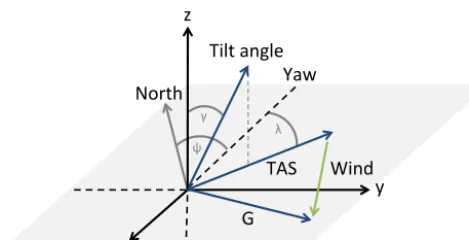
avi-Figure 3.Relationship between the tilt angleγ of the multicopter and the wind triangle with true air speed (TAS) vector, ground (G) vector and wind vector. Pitch angle is inxaxis and roll angle in yaxis direction. Yaw (ψ) is the viewing direction of the multicopter relative to north and the angle between TAS and yaw isλ.
ation authority, independent of area, altitude above ground and time of the day in the uncontrolled air space.
For vertical methane investigations close to the tower, a 40 cm long aluminum tube (3.2 mm outer diameter, 1.2 mm inner diameter) was installed on the multicopter with the inlet about 30 cm above the propellers. This was attached airtight to an additional sampling line (PTFE, 3.2 mm outer diame-ter, 2 mm inner diamediame-ter, 70 m long) and connected the CRD spectrometer and the multicopter. The 70 m sample line was flushed at a flow rate of 350 sccm min−1(calibrated for 0◦C and 1013.25 hPa) of which 200 sccm min−1 were drawn by the CRD analyzer. This resulted in a residence time of ap-proximately 38 s in the tube. At 50 m length, the tube was an additional payload of 650 g. Thus, the maximum ascent height was limited by the payload capacity of the multicopter. A fast thermocouple was installed for high-time-resolution air temperature measurements. The thermocouple used was a butt-welded type K (CHROMEGA®/ALOMEGA® CHAL-003, OMEGA, Stamford, CT, USA), one wire chromium nickel alloy and the other constantan, both with a diame-ter of 0.08 mm. Its measurement range was 0 to 60◦C with an output voltage of 50 mV per◦C. The response time was better than 1 Hz in calm air with an accuracy of ±0.1◦C. Calibration against a reference thermometer was done in the lab. Data were logged at 10 Hz. These data were also used together with pressure data from the autopilot for potential temperature (Tpot)calculations to get information about the
stability of the atmosphere. The used pressure sensor is a MS5611-01BA03 (AMSYS, Mainz, Germany) and is able to resolve an altitude of 10 cm corresponding to a precision of about±0.02 hPa.
2.3 Wind estimation
Multicopters move through the air by setting a tilt angle (γ )
towards the flying direction with the magnitude of tilt an-gle roughly proportional to speed. This anan-gle also changes to
compensate for wind variations during the flight. Therefore, without using an additional sensor for wind measurements, estimation of both horizontal wind speed and direction was possible with onboard sensors for the vehicle’s attitude con-trol by measuring the pitch (forwards and backwards), roll (left and right) and yaw (orientation to north) angles. In con-trast to an aircraft, which is controlled by setting a true air speed (TAS), a multicopter flies with a given ground speed, resulting in a varying TAS.
This relationship is shown in the wind triangle (Fig. 3). The ground (G) vector represents the speed and direction of the multicopter’s movement determined by the GPS, while the TAS vector represents the actual speed and direction to-wards which the multicopter is heading. The deviation of G and TAS is caused by the wind. Assuming hovering, the tilt angle is only a result of the wind and the TAS vector is con-trary to the ground vector. Consequently, in the easiest case the direction of TAS represents the horizontal wind direction and the length of the TAS vector the horizontal wind speed.
Equations applied for the wind calculation are based on Neumann and Bartholomai (2015) and explained in detail there. In this study, only vertical flights were investigated. First, the multicopter’s tilt angleγ was calculated from roll and pitch angles and then projected to thexy plane, which results in the TAS vector. Then, its direction was calculated relative to the viewing direction of the multicopter (yaw an-gle (ψ ))and is given by the angle λ. TAS direction and si-multaneous wind direction was determined by the sum ofψ
andλin case the TAS vector is on the right side of the view-ing direction ([ψ, ψ+180◦]). In the other case, this sum was subtracted from 360◦ and in both cases the result has to be within 0 and 360◦. Finally, the calculated tilt angle was
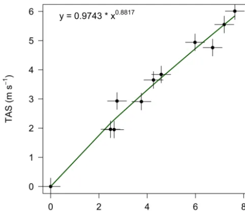
in-serted into a regression function to get the corresponding TAS. The length of the TAS vector represents the wind speed. Neumann and Bartholomai (2015) used wind tunnel ex-periments to determine the regression function. In contrast, in our approach the length of the TAS vector was determined by relating tilt angles to specific TASs during different flight experiments. The assumption was that without wind the TAS corresponds to the flight speed measured with the GPS (GPS speed or ground speed), which has an accuracy of 0.1 m s−1. The multicopter’s tilt angle was calculated by using pitch and roll angles. Their accuracy was better than 0.1◦. Using race-track flights, the regression function was experimentally de-termined during calm wind conditions with wind speeds be-low 1 m s−1. The track had a length of 120 m and had been flown six times on average for several ground speeds between 2 and 8 m s−1. While the ground speed was kept constant by
the GPS (<±0.2 m s−1), the variability of the assigned tilt angle was dependent on atmospheric conditions. To avoid an offset in the regression function the multicopter was balanced out. The resulting regression function is shown in Fig. 4 with the following Eq. (1):
Figure 4.Regression function of relationship between true air speed (TAS) and tilt angle (γ )experimentally determined with racetrack flights during calm wind conditions. The green line represents the fitted regression function and the error bars indicate the standard deviation of±0.4◦for the tilt angle and±0.3 m s−1, respectively.
The root-mean-square error (RMSE) of TAS determination was±0.3 m s−1. Based on this error for TAS, the RMSE of the tilt angle was±0.4◦, which is similar to the one of Neu-mann and Bartholomai (2015). This mean error of TAS leads to a higher relative error for low wind speeds than for higher wind speeds.
With this equation, horizontal wind speed and wind direc-tion were estimated from 1 Hz data and were averaged with a moving window over 10 s for further smoothing. To deter-mine the inaccuracy caused by a wind speed up to 1 m s−1 during the experimental flights, the variability of the tilt an-gle was analyzed during hovering under calm wind condi-tions (< 1 m s−1). This led to an uncertainty of 0.7±0.3◦, corresponding to a TAS of 0.7±0.3 m s−1, which resulted in an overall accuracy of TAS estimation of 0.7±0.6 m s−1.
2.4 Flight strategies
To demonstrate the functionality of the wind estimation based on the attitude control sensors of the multicopter, a comparison was done to a 3-D ultrasonic anemometer (uSonic3, Metek GmbH, Elmshorn, Germany) installed at a 9 m tower with an accuracy of 0.1 m s−1and 2◦at 5 m s−1. During windy conditions (3–5 m s−1)the multicopter hov-ered for 5 min close to the tower at a distance of approxi-mately 5 m. This horizontal distance as well as the 9 m height of the measurements ensured that the multicopter’s down-wash had an influence on neither the multicopter itself nor
the anemometer. For calm wind conditions, influences of the downwash were detected up to 5–6 m a.g.l.
In addition, vertical wind profiles were compared to other instruments such as lidar and sodar. The EC station was used as continuous time series information close to the ground. Reaching a height of 150 m a.g.l. with the multicopter, the range comparable to other instruments was about 100 m. For these flights, the vertical speed was set to 1.5 m s−1.
For methane measurements, the additional sampling line was attached to the multicopter and the spectrometer and was raised up to heights of 10, 25 and 50 m a.g.l. A hover time of 60 s at each level was included to get an averaged value. The pattern was repeated every 15 min. This led to a rotation of 5 min measurements with the multicopter and 10 min mea-surements at the tower at 1 m and 10 m a.g.l. For analysis, only the ascent data were used from the flights because there was no hovering during the descent. In addition, this strategy ensured that the multicopter did not mix the air before flying through. Alvarado et al. (2017) experimentally determined a distance of 40–45 cm above the multicopter, where the influ-ence of the rotors to air speed decreases significantly. So, the methane mixing ratio is actually not a point measurement but valid for a volume.
While most of the flights were done above the grassland site southwest of the EC station as shown in Fig. 1, the flights including methane measurements took place close to the methane tower in the southeast of the investigation area.
Time is given in UTC, which corresponds to CEST-2.
3 Results
3.1 Wind estimation
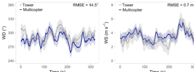
Information about the accuracy of the wind estimation was determined while hovering next to an ultrasonic anemometer with a distance of about 5 m (Fig. 5). The multicopter-derived wind direction showed a standard deviation of±11.1◦ and
multi-Figure 5.Wind direction (WD) and speed (WS) comparison between tower (grey) and multicopter (blue) at 9 m a.g.l. over 5 min. The colored bands around the lines represent the standard deviation of each time series.
copter should not be used as information about atmospheric turbulence.
In addition to the side-by-side measurements, wind esti-mation from vertical profiles was compared to lidar and sodar measurements as well as EC station data for near-ground in-formation (Fig. 6). Both lidar and EC station data (both 1 min time resolution) are shown for the time around the vertical profiles of the multicopter (∼4 min). The sodar had a tempo-ral resolution of 10 min, so only one value was available at each height. Wind direction and speed of the UAV data were in good agreement with the recordings of the different in-struments. During the flights at 09:01 and 09:31 UTC, wind direction was mainly from north to east with an increasing wind speed over time. For the first flight, spatial and tem-poral averages of multicopter, sodar and EC station were in agreement within 20–30◦and a standard deviation of about
±20◦for wind direction. Lidar data showed higher variabil-ity than other measurements but above 100 m data were in the same range. Wind speed for all instruments was low with an average of about 1–1.5 m s−1 and a standard devi-ation of about ±0.6 m s−1. For the second flight, the same was true for wind direction, but greater differences occurred for wind speed. While the multicopter and sodar recorded a mean speed of 2.6 and 2.5 m s−1, respectively, lidar and EC station had 1.7 and 1.4 m s−1, respectively. At this point it
has to be highlighted that the instruments were not located at the same place (distance 100–570 m from multicopter; see Fig. 1) and that time resolution varied. Besides, generation of turbulence from northeasterly winds is likely at the edge of the forest, which is to the east of the investigation area. Ac-cordingly, differences were explainable, especially at heights up to 50 m.
3.2 Methane and meteorological conditions
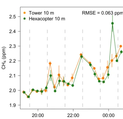
In the night between 21 and 22 July 2015, methane measure-ments were made with the multicopter starting about 15 min after sunset (19:05 UTC) and extending over 7 h (Fig. 7). For comparison of tower and multicopter results, the sub-sequent measurements are displayed with orange points for
tower data in 10 m and multicopter data with green ones also for 10 m. Short-term variations in methane concentra-tion were detected by both techniques, even with the same extent (around 22:00 UTC). There was only one major devi-ation shortly past midnight when the multicopter measured a value of 2.45 ppm compared to 2.2 ppm at the tower. This may be due to the distance of approx. 5 m between tower and UAV and a time difference of around 30 s between those measurements. Overall, the two data sets were significantly correlated with a Spearman correlation coefficient of 0.96. Calculation of the RMSE led to±0.063 ppm. Consequently, the measurements on the moving platform were as represen-tative as those of the stationary tower installation.
Considering the vertical methane profiles up to 50 m a.g.l., gradients were detectable during stable atmospheric condi-tions after sunset (Fig. 8). Data are shown for six flights with 1-hour intervals beginning at 19:32 UTC and ending at 00:32 UTC. According to the potential temperature profiles, a stable stratification of the atmosphere developed after sun-set indicated by increasing potential temperature with height. Its difference reached 5–6 K between ground and 50 m.
Thus, this overall stable stratification led to the reduced vertical mixing, and methane sources in the surround-ings caused a concentration rise of 0.3 ppm after sunset within 6 h. The mean background concentration measured during this campaign was 1.9 ppm. The concentration in-creased at each height with time, while accumulation started from the ground. Vertical gradients were already visible right after sunset and intensified until the measurement at 22:32 UTC, weakened afterwards and then intensified again at 00:32 UTC. This variability in varying gradients was in agreement with changing meteorological conditions. Mean concentrations averaged over all measurements at each level were 2.091 ppm (10 m), 2.049 ppm (25 m) and 1.976 ppm (50 m).
According to the continuous measurements at the tower, the CH4concentration increased close to the ground even
Sodar Lidar
Sodar Lidar
Sodar Lidar
Sodar Lidar
(a) (b)
Figure 6.Wind direction and speed profiles during two different flights: 09:01 UTC(a)and 09:31 UTC(b)on 15 July 2015. The blue profiles show multicopter data, dark grey circles represent EC station data, light grey squares lidar data and orange squares sodar data. Lidar and EC station data were averaged over the time the multicopter needed for the profile. Error bars show their standard deviation.
Figure 7.Methane mixing ratio measured at the tower and with the multicopter on the night between 21 and 22 July 2015. Tower data were measured just before the 10 m data from the multicopter. Error bars show the standard deviation for each measurement averaged over 60 s. A standard deviation of 0.01 ppm or less cannot be shown because the size of the data point exceeds the error bar. The dashed grey lines represent the time for which vertical profiles are shown in Figs. 8 and 9. Local time (CEST) is UTC+2.
at 25 m and 0.06 ppm at 50 m. Afterwards (23:32 UTC), con-centration decreased in 10 and 25 m and increased in 50 m, leading to almost the same concentration in all heights (ap-prox. 2.07 ppm).
Variations in agreement with a stabilization of the NBL were observed from the vertical potential temperature pro-files. The stability of the atmosphere increased, especially between 25 and 50 m until 22:32 UTC, while CH4
accumu-lated in the NBL. Below 25 m, the atmosphere was slightly stable to neutral. In the following hour, a destabilization in the lowest 50 m of the atmosphere was detected and after-wards stable conditions developed again. This destabilization occurred simultaneously with the mixing of methane at all heights followed by a reestablished methane gradient. The results indicated a developing surface layer up to 25 m a.g.l. where methane accumulated, but exchange with air above was not completely inhibited likely due to the fact that turbu-lence was not totally suppressed.
Wind in this night was mostly from west to northwest with low speed between 1 and 2 m s−1and up to 3 m s−1at 50 m (Fig. 9), and is shown for the same times as in Fig. 8. During the first 2 h, wind direction was roughly the same with height showing a variability of about 50◦(west to northwest), while wind speed was about 2–3 m s−1. Afterwards, wind speed
was lower at 10 and 25 m. Mean wind direction stayed be-tween west and northwest at 25 and 50 m, while at 10 m it changed from south (21:32 UTC) to west (22:32 UTC) and back to south and southwest (23:32 UTC). So, southern di-rections were accompanied by a methane decrease, lower wind speeds and higher potential temperature. In contrast to that, at 22:32 UTC wind speed was higher than 1 m s−1and potential temperature was 4–5 K lower than the hour before and after. During the last flight, wind direction changed back to northwest with high variability of about 100◦ at 10 and 25 m, which was not seen at the second height before. This higher variability occurred mostly during low wind speeds of 1–1.5 m s−1.
4 Discussion
Figure 8. Vertical potential temperature (Tpot)profiles in blue and methane concentrations in green over 6 h from 19:32 UTC (left) to
00:32 UTC (right) on the night of 21–22 July 2015. This corresponds to 21:32 to 02:32 CEST (UTC+2). Air temperature was measured with the thermocouple (ascent data only) andTpotwas calculated with the onboard pressure data from the autopilot.Tpotwas averaged at hovering
levels and smoothed with a moving average (3 s). Error bars of methane concentration show the standard deviation for each measurement averaged over 60 s. A standard deviation of 0.01 ppm or less cannot be shown because the size of the data point exceeds the error bar.
(a) (b)
Figure 9. Variability of wind direction(a)and speed (b) during 60 s hovering at 10, 25 and 50 m a.g.l. for flights between 19:32 and 00:32 UTC on the night of 21 to 22 July 2015. The blue box con-tains 50 % of the data and represents the interquartile range with the median as a black line. The dashed lines show maximum and minimum values in case those values are within the 1.5 interquar-tile range. Values outside this range (outliers) are represented with circles.
more flexible. Methane concentration measurements at 10 m height were in good agreement with those on the tower and could be conducted at different heights. Therefore, we con-clude that the technique of using a tube with a multicopter
could be also applicable for other inert trace gases and related research questions. In view of the good agreement of tower and UAV-based methane concentrations, plausible methane gradients were observed during stable atmospheric condi-tions although the multicopter does stir air with its propellers. Palomaki et al. (2017) demonstrated in an experiment that wind speed at 30 cm above the multicopter is 0.5 m s−1due to spinning rotors. According to Alvarado et al. (2017) this influence is negligible at a distance of 40–45 cm above the multicopter.
Methane concentration increases close to the ground were found below a nocturnal inversion. Using a tethered balloon instead of a multicopter, Choularton et al. (1995) detected a concentration drop of 0.05 to 0.075 ppm from the inver-sion layer to the layer above. This is in agreement with our multicopter measurements in 10 and 25 m a.g.l. being below 0.1 ppm in the first half of the night while a stable stratifica-tion occurred.
In addition, no influence of the tube on the tilt angle could be detected while hovering at 10, 25 and 50 m. A negligi-ble influence of payload was also found by Neumann and Bartholomai (2015). At each height, the multicopter had to lift more weight, but the autopilot compensated this with the spinning speed of the propellers, which was significantly higher on the side where the tube was mounted. Therefore, it is recommended to mount the tube in the center for a better flight performance. Besides, non-gusty wind conditions are favorable to reduce the wind load on the tube.
The wind estimation carried out during hovering showed good agreement with the tower with a RMSE of 14.5◦and 0.7 m s−1 for wind direction and speed, respectively. These values were determined using a moving average of 10 s. When applying a 20 s moving average, values of 12.5◦and 0.6 m s−1 are similar to those obtained by Neumann and Bartholomai (2015) for hovering. The advantage of our ap-proach is that no wind tunnel experiments are necessary and that the experimental flights are easy to reproduce. Since the estimated errors were a result of only a 5 min flight, further experiments and comparisons would be necessary to confirm these values. Our experimentally determined relationship be-tween TAS and the tilt angle is only valid for this hexacopter configuration and up to a speed of 6 m s−1.
Although the multicopter-based wind estimation was bi-ased, measurements showed similar results and the results of the other instruments showed differences too. Wind speed differed up to about 1 m s−1and direction up to 50◦ above 50 m. Below this height, influences of topography, land use and horizontal distance as well as averaging time were more pronounced and differences larger. Horizontal distance to the multicopter was 370 m for lidar and 540 m for sodar, while they had averaging times of 1 and 10 min, respec-tively, compared to the 10 s moving average of the multi-copter. Lothon et al. (2014), for example, found similar bi-ased differences dependent on horizontal distance and land use during the BLLAST campaign. In addition, low wind speeds (< 1 m s−1)lead to higher variability in wind direc-tion, as seen for lidar data. This is because the wind is not well coupled to the mesoscale flow, which often leads to vari-able wind directions (Anfossi et al., 2005; Mahrt, 2011). The same is true for multicopter-based wind direction at 10 m during the nighttime flights, which mainly occurred during wind speeds of less than 2 m s−1. With regard to wind es-timation from horizontal flights, this is especially important because flying with a specific speed requires a certain tilt an-gle. If this angle is significantly larger than the wind-induced angle, determination of wind contribution to the angle could be more difficult depending on the accuracy of measuring the angle.
Hovering close to the ground led to limitations in the es-timation of wind from the flight control sensors. The pro-peller’s downwash caused motion of air beneath the multi-copter. These were compensated by changing the tilt angle but did not reflect actual wind conditions below a height of
5–6 m a.g.l. The effect was stronger during calm conditions because the jet of perturbed air did not advect away effec-tively. For the same reason, the data collected during descent were not used to estimate wind conditions because the mul-ticopter moved through its own downwash.
Since the thermocouple was placed below a rotor, disconti-nuities were found while hovering; the temperature measure-ment is representative of the volume around the multicopter rather than a point. But this ensured a continuous flow around the sensor, which increased its response time. For analysis, temperature was averaged for hovering at each level during the methane measurements.
The combination of the wind and concentration measure-ments suggest that the significant methane increase between 21:32 and 22:32 UTC was caused by emissions from the dairy farms (about 150–200 dairy cows) to the west of the measurement location (about 600 m distance). Actually, the methane mixing ratio started to increase around 22:00 UTC (Fig. 7), when wind direction changed from more southern to predominating western directions (250–300◦) with wind speeds of around 1.5 m s−1(Fig. 9). Below 25 m, the atmo-sphere was mixed according to the vertical potential temper-ature profile. Taking into account these conditions, disper-sion of a methane plume is low. According to Dämmgen et al. (2012), an emission rate of 14.5 g h−1cow−1 can be as-sumed. This value was estimated for dairy cows in Bavaria (Germany) based on the IPCC guidelines (2006). Depending on the width of the methane plume(s) (100–500 m) coming from the farms, the methane concentration increase of about 0.15 ppm in 30 min would lead to emissions from about 90 to 450 cows. In comparison to the actual number of dairy cows measured methane concentrations were plausible. For further investigation, an approach similar to that of Hacker et al. (2016) would be suitable to calculate emission rates by flying upwind and downwind of the farms and measuring the vertical and horizontal extent of the plume.
5 Conclusion and outlook
and aerosols in the air. However, to apply budget methods for ground flux estimations as discussed by Denmead et al. (2000), the vertical coverage needs to be extended, for example by utilization of a lightweight onboard methane sen-sor.
Also for horizontal methane investigations, a lightweight and small methane sensor on board a multicopter would be beneficial. With such a sensor it would become possible to investigate the size of the methane plumes horizontally and vertically and determine methane fluxes. Besides, the inves-tigation of further methane sources and sinks as well as their strengths is planned in that area. To this end, horizontal wind estimation is necessary.
Data availability. Data from the ScaleX-2015 campaign are freely
available for participants and upon request for third parties.
Competing interests. The authors declare that they have no conflict
of interest.
Acknowledgements. This research was supported by the
TER-restrial Environmental Observatory (TERENO) pre-Alpine infrastructure funded by the Helmholtz Association and the Federal Ministry of Education and Research as well as the Ground Truth Demo and Test Facilities (ACROSS) infrastructure funded by the Helmholtz Association. The corresponding author was partly supported by a scholarship of the GRAduate School of Climate and Environment (GRACE) of the Karlsruhe Institute of Technology (KIT). Their support is highly acknowledged. We also thank the Scientific Team of the ScaleX-2015 campaign for their contribution.
The article processing charges for this open-access publication were covered by a Research
Centre of the Helmholtz Association.
Edited by: Eric C. Apel
Reviewed by: Jens Bange and two anonymous referees
References
Altstädter, B., Platis, A., Wehner, B., Scholtz, A., Wildmann, N., Hermann, M., Käthner, R., Baars, H., Bange, J., and Lampert, A.: ALADINA – an unmanned research aircraft for observing vertical and horizontal distributions of ultrafine particles within the atmospheric boundary layer, Atmos. Meas. Tech., 8, 1627– 1639, https://doi.org/10.5194/amt-8-1627-2015, 2015.
Alvarado, M., Gonzalez, F., Fletcher, A., and Doshi, A.: Towards the Development of a Low Cost Airborne Sensing System to Monitor Dust Particles after Blasting at Open-Pit Mine Sites, Sensors, 15, 19667–19687, https://doi.org/10.3390/s150819667, 2015.
Alvarado, M., Gonzales, F., Erskine, P., Cliff, D., and Heuff, D.: A Methodology to Monitor Airborne PM10 Dust Particles
Using a Small Unmanned Aerial Vehicle, Sensors, 17, 343, https://doi.org/10.3390/s17020343, 2017.
Andrews, A. E., Kofler, J. D., Trudeau, M. E., Williams, J. C., Neff, D. H., Masarie, K. A., Chao, D. Y., Kitzis, D. R., Novelli, P. C., Zhao, C. L., Dlugokencky, E. J., Lang, P. M., Crotwell, M. J., Fischer, M. L., Parker, M. J., Lee, J. T., Baumann, D. D., Desai, A. R., Stanier, C. O., De Wekker, S. F. J., Wolfe, D. E., Munger, J. W., and Tans, P. P.: CO2, CO, and CH4measurements from tall
towers in the NOAA Earth System Research Laboratory’s Global Greenhouse Gas Reference Network: instrumentation, uncer-tainty analysis, and recommendations for future high-accuracy greenhouse gas monitoring efforts, Atmos. Meas. Tech., 7, 647– 687, https://doi.org/10.5194/amt-7-647-2014, 2014.
Anfossi, D., Oetti, D., Degrazia, G., and Goulart A.: An analysis of sonic anemometer observations in low wind speed conditions, Bound.-Lay. Meteorol., 114, 179–203, https://doi.org/10.1007/s10546-004-1984-4, 2005.
Bamberger, I., Stieger, J., Buchmann, N., and Eugster, W.: Spatial variability of methane: Attributing atmospheric concentrations to emissions, Environ. Pollut., 190, 65–74, https://doi.org/10.1016/j.envpol.2014.03.028, 2014.
Banta, R. M., Pichugina, Y. L., Kelley, N. D., Hardesty, R. M., and Brewer, W. A.: Wind energy meteorology: Insight into wind properties in the turbine-rotor layer of the atmosphere from high-resolution Doppler lidar, B. Am. Meteorol. Soc., 94, 883–902, https://doi.org/10.1175/BAMS-D-11-00057.1, 2013.
Båserud, L., Reuder, J., Jonassen, M. O., Kral, S. T., Paskyabi, M. B., and Lothon, M.: Proof of concept for turbulence measure-ments with the RPAS SUMO during the BLLAST campaign, At-mos. Meas. Tech., 9, 4901–4913, https://doi.org/10.5194/amt-9-4901-2016, 2016.
Berman, E. S. F., Fladeland, M. L. J., Kolyer, R., and Gupta, M.: Greenhouse gas analyzer for measurements of carbon dioxide, methane, and water vapor aboard an un-manned aerial vehicle, Sensor. Actuat. B-Chem., 169, 128–135, https://doi.org/10.1016/j.snb.2012.04.036, 2012.
Beswick, K. M., Simpson, T. W., Fowler, D., Choularton, T. W., Gallagher, M. W., Hargreaves, K. J., Sutton, M. A., and Kaye, A.: Methane emissions on large scales, Atmos. Environ., 32, 3283– 3291, https://doi.org/10.1016/S1352-2310(98)00080-6, 1998. Chang, C.-C., Wang, J.-L., Chang, C.-Y., and Liang, M.-C.:
Devel-opment of a multicopter-carried whole air sampling apparatus and its applications in environmental studies, Chemosphere, 144, 484–492, https://doi.org/10.1016/j.chemosphere.2015.08.028, 2016.
Choularton, T. W., Gallagher, M. W., Bower, K. N., Fowler, D., Zah-niser, M., and Kaye, A.: Trace Gas Flux Measurements at the Landscape Scale Using Boundary-Layer Budgets, Phil. Trans. Roy. Soc. A., 351, 357–369, 1995.
Dämmgen, U., Rösemann, C., Haenel, H.-D., and Hutchings, N. J.: Enteric methane emissions from German dairy cows, Landbau-forsch. Appl. Agric. Forestry Res., 1/2, 21–32, 2012.
Denmead, O. T., Leuning, R., Griffith, D. W. T., Jamie, I. M., Esler, M. B., Harper, L. A., and Freney, J. R.: Verifying in-ventory predictions of animal methane emissions with meteo-rological measurements, Bound.-Lay. Meteorol., 69, 187–209, https://doi.org/10.1023/A:1002604505377, 2000.
Dlugokencky, E. J., Nisbet, E. G., Fisher, R., and Lowry, D.: Global atmospheric methane: budget, changes and dangers, Phil. Trans. R. Soc. A., 369, 2058–2072, https://doi.org/10.1098/rsta.2010.0341, 2011.
Egger, J., Bajrachaya, S., Heinrich, R., Kolb, P., Lämmlein, S., Mech, M., Reuder, J., Schäper, W., Shakya, P., Schween, J., and Wendt, H.: Diurnal winds in the Himalayan Kali Gandaki val-ley. Part III: Remotely piloted aircraft soundings, Mon. Weather Rev., 130, 2042–2058, 2002.
Emeis, S., Schäfer, K., and Münkel, C.: Observation of the struc-ture of the urban boundary layer with different ceilometers and validation by RASS data, Meteorol. Z., 18, 149–154, https://doi.org/10.1127/0941-2948/2009/0365, 2009.
Forster, P., Ramaswamy, V., Artaxo, P., Berntsen, T., Betts, R., Fa-hey, D. W., Haywood, J., Lean, J., Lowe, D. C., Myhre, G., Nganga, J., Prinn, R., Raga, G., Schulz, M., and Van Dorland, R.: Changes in Atmospheric Constituents and in Radiative Forc-ing, in: Climate Change 2007: The Physical Science Basis. Con-tribution of Working Group I to the Fourth Assessment Report of the Intergovernmental Panel on Climate Change, edited by: Solomon, S., Qin, D., Manning, M., Chen, Z., Marquis, M., Av-eryt, K. B., Tignor, M., and Miller, H. L., Cambridge University Press, Cambridge, United Kingdom and New York, NY, USA, 2007.
Hacker, J. M., Chen, D., Bai, M., Ewenz, C., Junkermann, W., Lieff, W., McManus, B., Neininger, B., Sun, J., Coates, T., Denmead, T., Flesch, T., McGinn, S., and Hill, J.: Using airborne technol-ogy to quantify and apportion emissions of CH4and NH3from
feedlots, Anim. Prod. Sci., 56, 190–203, 2016.
Hammann, E., Behrendt, A., Le Mounier, F., and Wulfmeyer, V.: Temperature profiling of the atmospheric boundary layer with rotational Raman lidar during the HD(CP)2Observational Prototype Experiment, Atmos. Chem. Phys., 15, 2867–2881, https://doi.org/10.5194/acp-15-2867-2015, 2015.
Holland, G. J., McGeer, T., and Youngren, H.: Autonomous aerosondes for economical atmospheric soundings anywhere on the globe, B. Am. Meteor. Soc., 73, 1987–1998, 1992.
IPCC – Intergovernmental Panel on Climate Change: 2006 IPCC guidelines for national greenhouse gas inventories, Vol. 4: Agriculture, forestry and other land use, Chap-ter 10, http://www.ipcc-nggip.iges.or.jp/public/2006gl/pdf/4_ Volume4/V4_10_Ch10_Livestock.pdf (last access: 21 June 2017), 2006.
Khan, A., Schaefer, D., Tao, L., Miller, D. J., Sun, K., Zondlo, M. A., Harrison, W. A., Roscoe, B., and Lary, D. J.: Low Power Greenhouse Gas Sensors for Unmanned Aerial Vehicles, Remote Sens., 4, 1355–1368, https://doi.org/10.3390/rs4051355, 2012. Kirschke, S., Bousquet, P., Ciais, P., Saunois, M., Canadell, J. G.,
Dlugokencky, E. J., Bergamaschi, P., Bergmann, D., Blake, D. R., Bruhwiler, L., Cameron-Smith, P., Castaldi, S., Chevallier, F., Feng, L., Fraser, A., Heimann, M., Hodson, E. L., Houwel-ing, S., Josse, B., Fraser, P. J., Krummel, P. B., Lamarque, J. F., Langenfelds, R. L., Le Quere, C., Naik, V., O’Doherty, S., Palmer, P. I., Pison, I., Plummer, D., Poulter, B., Prinn, R. G.,
Rigby, M., Ringeval, B., Santini, M., Schmidt, M., Shindell, D. T., Simpson, I. J., Spahni, R., Steele, L. P., Strode, S. A., Sudo, K., Szopa, S., Van Der Werf, G. R., Voulgarakis, A., Van Weele, M., Weiss, R. F., Williams, J. E., and Zeng, G.: Three decades of global methane sources and sinks, Nat. Clim. Change, 6, 813– 823, https://doi.org/10.1038/NGEO1955, 2013.
Konrad, T., Hill, M., Rowland, J., and Meyer J.: A small, radio-controlled aircraft as a platform for meteorological sensors, Appl. Phys. Lab. Tech. Digest, 10, 11–19, 1970.
Korhonen, K., Giannakaki, E., Mielonen, T., Pfüller, A., Laakso, L., Vakkari, V., Baars, H., Engelmann, R., Beukes, J. P., Van Zyl, P. G., Ramandh, A., Ntsangwane, L., Josipovic, M., Ti-itta, P., Fourie, G., Ngwana, I., Chiloane, K., and Komp-pula, M.: Atmospheric boundary layer top height in South Africa: measurements with lidar and radiosonde compared to three atmospheric models, Atmos. Chem. Phys., 14, 4263–4278, https://doi.org/10.5194/acp-14-4263-2014, 2014.
Kunstmann, H., Schneider, K., Forkel, R., and Knoche, R.: Impact analysis of climate change for an Alpine catchment using high resolution dynamic downscaling of ECHAM4 time slices, Hydrol. Earth Syst. Sci., 8, 1031–1045, https://doi.org/10.5194/hess-8-1031-2004, 2004.
Kunstmann, H., Krause, J., and Mayr, S.: Inverse distributed hydro-logical modelling of Alpine catchments, Hydrol. Earth Syst. Sci., 10, 395–412, https://doi.org/10.5194/hess-10-395-2006, 2006. Lothon, M., Lohou, F., Pino, D., Couvreux, F., Pardyjak, E. R.,
Reuder, J., Vilà-Guerau de Arellano, J., Durand, P., Hartogensis, O., Legain, D., Augustin, P., Gioli, B., Lenschow, D. H., Faloona, I., Yagüe, C., Alexander, D. C., Angevine, W. M., Bargain, E., Barrié, J., Bazile, E., Bezombes, Y., Blay-Carreras, E., van de Boer, A., Boichard, J. L., Bourdon, A., Butet, A., Campistron, B., de Coster, O., Cuxart, J., Dabas, A., Darbieu, C., Deboudt, K., Delbarre, H., Derrien, S., Flament, P., Fourmentin, M., Garai, A., Gibert, F., Graf, A., Groebner, J., Guichard, F., Jiménez, M. A., Jonassen, M., van den Kroonenberg, A., Magliulo, V., Martin, S., Martinez, D., Mastrorillo, L., Moene, A. F., Molinos, F., Moulin, E., Pietersen, H. P., Piguet, B., Pique, E., Román-Cascón, C., Rufin-Soler, C., Saïd, F., Sastre-Marugán, M., Seity, Y., Steen-eveld, G. J., Toscano, P., Traullé, O., Tzanos, D., Wacker, S., Wildmann, N., and Zaldei, A.: The BLLAST field experiment: Boundary-Layer Late Afternoon and Sunset Turbulence, Atmos. Chem. Phys., 14, 10931–10960, https://doi.org/10.5194/acp-14-10931-2014, 2014.
Mahrt, L.: Surface Wind Direction Variability, J. Appl. Meteorol. Clim., 50, 144–152, https://doi.org/10.1175/2010JAMC2560.1, 2011.
Martin, S., Bange, J., and Beyrich, F.: Meteorological profiling of the lower troposphere using the research UAV “M2AV Carolo”, Atmos. Meas. Tech., 4, 705–716, https://doi.org/10.5194/amt-4-705-2011, 2011.
Mathieu, N., Strachan, I. B., Leclerc, M. Y., Karipot, A., and Pat-tey, E.: Role of low-level jets and boundary-layer properties on the NBL budget technique, Agr. Forest Meteorol., 135, 35–43, https://doi.org/10.1016/j.agrformet.2005.10.001, 2005.
McGeer, T. and Holland, G.: Small autonomous aircraft for eco-nomical oceanographic observations on a wide scale, Oceanog-raphy, 6, 129–135, 1993.
Nathan, B. J., Golston, L. M., O’Brien, A. S., Ross, K., Harri-son, W. A., Tao, L., Lary, D. J., JohnHarri-son, D. R., Covington, A. N., Clark, N. N., and Zondlo, M.: Near-field characteriza-tion of methane emission variability from a compressor stacharacteriza-tion using a model aircraft, Environ. Sci. Technol., 49, 7896–7903, https://doi.org/10.1021/acs.est.5b00705, 2015.
Neumann, P. P. and Bartholomai, M.: Real-time wind estima-tion on a micro unmanned aerial vehicle using its inertial measurement unit, Sensor Actuat. A-Phys., 235, 300–310, https://doi.org/10.1016/j.sna.2015.09.036, 2015.
Palomaki, R. T., Rose, N. T., van den Bossche, M., Sherman, T. J., and De Wekker, S. F. J.: Wind Estimation in the Lower At-mosphere Using Multirotor Aircraft, Atmos. Ocean. Tech., 34, 1183–1191, https://doi.org/10.1175/JTECH-D-16-0177.1, 2017. Rennó, N. O. and Williams, E. R.: Quasi-lagrangian measurements in convective boundary layer plumes and their implications for the calculation of cape, Mon. Weather Rev, 123, 2733–2742, 1995.
Sasakawa, M., Shimoyama, K., Machida, T., Tsuda, N., Suto, H., Arshinov, M., Davydov, D., Fofonov, A., Krasnov, O., Saeki, T., Koyama, Y., and Maksyutov, S.: Continuous measurements of methane from a tower network over Siberia, Tellus B, 62, 403– 416, https://doi.org/10.1111/j.1600-0889.2010.00494.x, 2010. Saunois, M., Jackson, R. B., Bousquet, P., Poulter, B., and
Canadell, J. G.: The growing role of methane in anthro-pogenic climate change, Environ. Res. Lett., 11, 120207, https://doi.org/10.1088/1748-9326/11/12/120207, 2016. Soddell, J. R., McGuffie, K., and Holland, G. J.: Intercomparison
of atmospheric soundings from the aerosonde and radiosondes, J. Appl. Meteor. Climatol., 43, 1260–1269, 2004.
Spiess, T., Bange, J., Buschmann, M., and Vörsmann, P.: First ap-plication of the meteorological Mini-UAV “M2AV”, Meteorol. Z., 16, 159–169, https://doi.org/10.1127/0941-2948/2007/0195, 2007.
Stieger, J., Bamberger, I., Buchmann, N., and Eugster, W.: Vali-dation of farm-scale methane emissions using nocturnal bound-ary layer budgets, Atmos. Chem. Phys., 15, 14055–14069, https://doi.org/10.5194/acp-15-14055-2015, 2015.
Stull, R.: An Introduction to Boundary Layer Meteorology, 9th Edn., Dordrecht, 1988.
Velasco, E., Márquez, C., Bueno, E., Bernabé, R. M., Sánchez, A., Fentanes, O., Wöhrnschimmel, H., Cárdenas, B., Kamilla, A., Wakamatsu, S., and Molina, L. T.: Vertical distribution of ozone and VOCs in the low boundary layer of Mexico City, Atmos. Chem. Phys., 8, 3061–3079, https://doi.org/10.5194/acp-8-3061-2008, 2008.
Villa, T. F., Gonzalez, F., Miljievic, B., Ristovski, Z. D., and Morawska, L.: An Overview of Small Unmanned Aerial Vehicles for Air Quality Measurements: Present Applications and Future Prospectives, Sensors, 16, 1072, https://doi.org/10.3390/s16071072, 2016.
Wang, J. M., Murphy, J. G., Geddes, J. A., Winsborough, C. L., Basiliko, N., and Thomas, S. C.: Methane fluxes measured by eddy covariance and static chamber techniques at a temperate forest in central Ontario, Canada, Biogeosciences, 10, 4371– 4382, https://doi.org/10.5194/bg-10-4371-2013, 2013.
Wolf, B., Chwala, C., Fersch, B., Garvelmann, J., Junkermann, W., Zeeman, M., Angerer, A., Adler, B., Beck, C., Brosy, C., Brugger, P., Emeis, S., Dannenmann, M., De Roo, F., Diaz-Pines, E., Haas, E., Hagen, M., Hajnsek, I., Jacobeit, J., Jagdhu-ber, T., Kalthoff, N., Kiese, R., Kunstmann, H., Kosak, O., Krieg, R., Malchow, C., Mauder, M., Merz, R., Notarnicola, C., Philipp, A., Reif, W., Reineke, S., Rödiger, T., Ruehr, N., Schäfer, K., Schrön, M., Senatore, A., Shupe, H., Völksch., I., Wanninger, C., Zacharias, S., and Schmid, H. P.: The ScaleX campaign: scale-crossing land-surface and boundary layer pro-cesses in the TERENO-preAlpine observatory, B. Am. Me-teor. Soc., 98, 1217–1234, https://doi.org/10.1175/BAMS-D-15-00277.1, 2017.
Worden, J., Kulawik, S., Frankenberg, C., Payne, V., Bowman, K., Cady-Peirara, K., Wecht, K., Lee, J.-E., and Noone, D.: Profiles of CH4, HDO, H2O, and N2O with improved lower
tropospheric vertical resolution from Aura TES radiances, At-mos. Meas. Tech., 5, 397–411, https://doi.org/10.5194/amt-5-397-2012, 2012.
Zacharias, S., Bogena, H., Samaniego, L., Mauder, M., Fuß, R., Pütz, T., Frenzel, M., Schwank, M., Baessler, C., Butterbach-Bahl, K., Bens, O., Borg, E., Brauer, A., Dietrich, P., Hajnsek, I., Helle, G., Kiese, R., Kunstmann, H., Klotz, S., Munch, J. C., Papen, H., Priesack, E., Schmid, H. P., Steinbrecher, R., Rosen-baum, U., Teutsch, G., and Vereecken, H.: A Network of Terres-trial Environmental Observatories in Germany, Vadose Zone J., 10, 955–973, https://doi.org/10.2136/vzj2010.0139, 2011. Zeeman, M. J., Mauder, M., Steinbrecher, R., Heidbach, K., Eckart,