www.ocean-sci.net/5/461/2009/
© Author(s) 2009. This work is distributed under the Creative Commons Attribution 3.0 License.
Ocean Science
A nested Atlantic-Mediterranean Sea general circulation model for
operational forecasting
P. Oddo1, M. Adani1, N. Pinardi2, C. Fratianni1, M. Tonani1, and D. Pettenuzzo1
1Gruppo Nazionale di Oceanografia Operativa, Istituto Nazionale di Geofisica e Vulcanologia, Via Aldo Moro 44, 40128 Bologna, Italy
2Centro Interdipartimentale per la Ricerca in Scienze Ambientali, Universit`a di Bologna Ravenna, Italy Received: 25 May 2009 – Published in Ocean Sci. Discuss.: 15 June 2009
Revised: 7 September 2009 – Accepted: 6 October 2009 – Published: 26 October 2009
Abstract. A new numerical general circulation ocean model for the Mediterranean Sea has been implemented nested within an Atlantic general circulation model within the framework of the Marine Environment and Security for the European Area project (MERSEA, Desaubies, 2006). A 4-year twin experiment was carried out from January 2004 to December 2007 with two different models to evaluate the impact on the Mediterranean Sea circulation of open lateral boundary conditions in the Atlantic Ocean. One model con-siders a closed lateral boundary in a large Atlantic box and the other is nested in the same box in a global ocean circula-tion model. Impact was observed comparing the two simula-tions with independent observasimula-tions: ARGO for temperature and salinity profiles and tide gauges and along-track satellite observations for the sea surface height. The improvement in the nested Atlantic-Mediterranean model with respect to the closed one is particularly evident in the salinity characteris-tics of the Modified Atlantic Water and in the Mediterranean sea level seasonal variability.
1 Introduction
Simulating and forecasting Mediterranean Sea dynamics is challenging due to the very complex dynamics characteriz-ing this semi-enclosed deep basin. In the past ten years, op-erational oceanography has become a reality in the Mediter-ranean Sea: the regional implementation plan (Pinardi and Flemming, 1998) has been accomplished and integrated ob-servation and modelling has been carried out producing real time daily forecasts with multivariate data assimilation and
Correspondence to: P. Oddo
nesting of sub-regional and shelf models (Pinardi et al., 2003). Operational modelling for forecasting allows contin-uous and quantitative assessment of the quality of the model simulations and this is expected to serve as the test bed for the development of new model solutions and parameteriza-tions. This paper illustrates a major step in modelling the Mediterranean Sea, never before carried out, which consid-ers one-way nesting in the Atlantic ocean with a global ocean forecasting system developed during the MERSEA project (Desaubies, 2006). Previous models of the Mediterranean Sea circulation have parameterized the connection with the Atlantic ocean in different ways (i.e., Tonani et al., 2008; Beranger et al., 2005) but none of them has demonstrated the sensitivity of the simulated Mediterranean circulation to the coupling with the Atlantic.
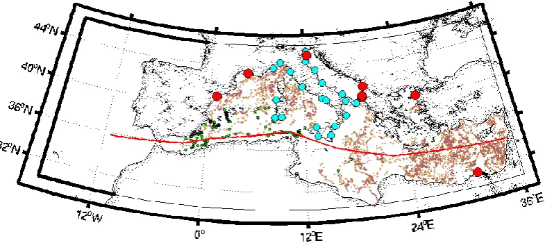
Fig. 1. Model domain. Bold lines in the Atlantic indicate location of model lateral boundaries. Red circles indicate river locations and the
Dardanelles inflow. Dots (red and dark green) indicate ARGO float positions. The dark green dots indicate position of the ARGO floats sampling the inflowing Atlantic Water. Cyan dots indicate the position of tide gauges. Red line indicates the cross section shown in Fig. 4.
the main component of the Mediterranean outflow to the Atlantic. LIW also provides a preconditioning mechanism for the Eastern Mediterranean Deep Water (EMDW) and the Western Mediterranean Deep Water (WMDW), the two lo-cally formed deep waters of the basin.
Moreover, the horizontal circulation structure is rather complex, consisting of mesoscale and sub-basin scale gyre structures. Permanent, recurrent and transitional cyclonic and anticyclonic gyres and eddies, influenced by bathymetric features are interconnected by currents and jets (Robinson et al., 1994; Pinardi et al., 2006). The complexity of the circu-lation is due to the special combination of the surface forc-ing with the lateral fluxes imposed by water exchanges at the Gibraltar Strait. It is therefore important to show the sensitiv-ity of the circulation to the Atlantic-Mediterranean coupling and two approaches are compared in this paper. The first con-sists of a consolidated modelling approach (Roussenov et al., 1995; Demirov and Pinardi, 2002; Tonani et al., 2008) where a large Atlantic box is considered with closed boundaries and relaxation to climatology for the temperature and salin-ity tracers. Gibraltar is explicitly resolved by the model but the Atlantic is heavily parameterized. The second consists of one-way, state-of-the-art nesting of a limited area general circulation model in a global scale model (Marchesiello et al., 2001; Oddo and Pinardi, 2008). Other approaches have been used in the past, most of them use a limited buffer zone in the Atlantic where temperature and salinity are re-laxed to seasonal data, observation- or model-derived (Be-ranger et al., 2005; Testor et al., 2005; Bozec et al., 2006). The final objective of this paper is to show how two differ-ent Atlantic-Mediterranean coupling methods influence the Mediterranean Sea circulation.
Section 2 describes the general circulation model imple-mentation. Model results and comparison with observations
are discussed in Sects. 3 and 4. Section 5 offers summary and conclusions.
2 Ocean model description
The present Mediterranean operational model, hereafter called MFS V1, is an implicit free-surface version of the Ocean PArallelise code (OPA, Madec et al., 1998) with a 1/16◦-degree horizontal regular resolution and 72 unevenly spaced vertical z-levels (Tonani et al., 2008). In this paper we describe a new model implementation carried out with the same horizontal and vertical regional boundaries but based on a new OPA code (OPA 9.0 Madec, 2008), hereafter called MFS V2. Only the differences with the earlier system will be described here in any detail.
MFS V2 covers the entire Mediterranean Sea and also ex-tends into the Atlantic (see Fig. 1) with the same horizon-tal and vertical resolution of MFS V1. However, MFS V2 uses vertical partial cells to fit the bottom depth shape. Like MFS V1, the model is forced by momentum, water and heat fluxes interactively computed by bulk formulae using the 6-h, 0.5◦horizontal-resolution operational analyses from the European Centre for Medium-Range Weather Forecasts (ECMWF) and model predicted surface temperatures (de-tails of the air-sea physics are in Tonani et al., 2008). The only difference in the bulk formula concerns the calculation of the latent heat flux; in the previous model implementation constant turbulent exchange coefficients were used, while in the model presented here they vary according to the empiric formula suggested by Kondo (1975).
natural surface boundary condition for vertical velocity: w z
=h−
∂h
∂t +v· ∇h
z=h
= −
E−P − R
FR
(1) wherewis the vertical velocity,his the surface elevation,E
is the evaporation in m s−1,Pis the precipitation in m s−1,R
indicates the rivers runoff in m3s−1andFR the river mouth
discharge area. The complementary salt flux boundary con-dition is also:
Ak ∂S ∂z
z=h
=Sz=h
E−P − R
FR
(2) where Ak is the vertical turbulent diffusion coefficient in
m2s−1 andSz=h is the model surface salinity in PSU. In
MFS V1 the water flux, E−P−R
FR
, was estimated by means of a relaxation to surface climatological salinity (To-nani et al., 2008). In MFS V2,Eis derived from the latent heat flux;P is taken from monthly mean Climate Prediction Center Merged Analysis of Precipitation (CMAP) Data (Xie and Arkin, 1997) andR is composed of monthly mean cli-matological data. Only seven major rivers have been imple-mented (Fig. 1): the Ebro, Nile and Rhone monthly values are from the Global Runoff Data Centre (Fekete et al., 1999) and the Adriatic rivers (Po, Vjos¨e, Seman and Bojana) are from Raicich (Raicich, 1996). In this model configuration the Dardanelles inflow has been parameterized as a river and its monthly climatological net inflow rates were taken from Kourafalou and Barbopoulos (2003).
The advection scheme for active tracers (temperature and salinity) has been modified, replacing the 2nd order cen-tered advection (MFS V1) with a mixed up-stream/MUSCL (Monotonic Upwind Scheme for Conservation Laws, Van Leer, 1979, as implemented by Estubier and L´evy, 2000) scheme. This flux-limiting scheme is particularly suitable for operational purposes not only because it is able to preserve gradients without significant numerical noise, but also be-cause it has the capability to switch, without additional com-putational cost, to a simple up-stream scheme in areas where numerical instabilities can occur. The up-stream scheme is used in proximity of the river mouths, in the Gibraltar Strait and close to the Atlantic lateral boundaries. This “diffusive” advection scheme is used to simulate a “sponge layer” in or-der to avoid numerical overshooting due to large horizontal and/or vertical gradients deriving from the fresh water runoff and to numerical discontinuities due to the only partially ex-act imposition of lateral boundary conditions. At Gibraltar, the up-stream scheme, together with an artificially increased vertical diffusivity (similar to MFS V1 implementation), pa-rameterizes the large mixing acting in this area due to the internal wave and tide breaking, which is not explicitly re-solved by the model (tidal dynamics is not implemented in both MFS V1 and MFS V2).
The major model improvement discussed in this paper concerns the parameterization of the connection between
the Mediterranean Sea and the North Atlantic Ocean. In MFS V1, the Atlantic part of the model consisted of three closed boundaries where, in order to keep the solution re-alistic, the temperature and salinity were relaxed toward monthly climatological values (Levitus, 1998) using a space dependent relaxation function. In the same area a sponge layer was also implemented in order to reduce the numer-ical noise (Tonani et al., 2008). In MFS V2, the Atlantic box is nested within the monthly mean climatological fields computed from the daily output of the1/4×1/4degrees global model, hereafter called MERCATOR-1/4 (Drevillon et al., 2008), spanning from 2001 to 2005.
In order to understand and quantify the improvements de-riving from the nested approach better, two different im-plementations of the new model are considered in this study: in the first (MFS V2.1) the same parameterization as MFS V1 has been adopted in the Atlantic area; in the second (MFS V2.2) the model has been nested into the global model using a lateral open boundary condition approach.
In the MFS V2.2 model, the 2-D adaptive radiation con-dition (Marchesiello et al., 2001; Oddo and Pinardi, 2008) has been used for the active tracers. Total velocities at the open boundaries are imposed from the global model solution, while barotropic velocities use a modified Flather (1976) lateral boundary condition explained in Oddo and Pinardi (2008). The nested normal total velocity,u, imposed at the lateral open boundaries, is:
u=uext−uext
1−H+η
ext
H+η
+ C
H+η η−η
ext (3)
whereuextandηextare the total velocity and the surface el-evation prescribed by the nesting global model respectively,
Cis the phase velocity calculated using an Orlanski formula-tion (Orlanski, 1976),ηis the nested model free surface and
uextis the vertically integrated (barotropic) velocity defined as follows:
uext= 1
H+ηext
ηext
Z
−H
uextdz.
Using a closed domain model (MFS V2.1), particular atten-tion should be given to volume conservaatten-tion in the presence of the natural vertical boundary condition (1). Here we use the same approach described in Tonani et al. (2008) to correct the surface water flux in the Atlantic-Mediterranean closed model domain. The model surface mean of the water flux,
E−P−R
FR
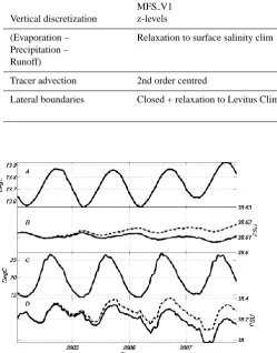
Table 1. Major differences between the previous Mediterranean Forecasting System (MFS) model implementation and the two new versions
analyzed in this study: MFSV2.1, closed domain ; MFS V2.2 open domain.
MFS V1 MFS V2.1 MFS V2.2
Vertical discretization z-levels z-levels +partial cells z-levels +partial cells
(Evaporation – Precipitation – Runoff)
Relaxation to surface salinity clim Interactively computed CMAP precipitation Clim runoff
Interactively computed CMAP precipitation Clim runoff
Tracer advection 2nd order centred MUSCL + up-stream MUSCL + up-stream
Lateral boundaries Closed + relaxation to Levitus Clim Closed + relax to MERCA-TOR
Open – nested with MER-CATOR
Fig. 2. (A) Time series of mean volume temperature. Solid (MFS V2.1) and dashed (MFS V2.2) lines overlap. (B) Time se-ries of mean volume salinity, solid line indicates MFS V2.1 re-sults, dashed line indicates MFS V2.2 results. (C) Time series of mean surface temperature, solid line (MFS V2.1) and dashed (MFS V2.2) lines overlap. (D) Time series of mean surface salin-ity, solid line indicates MFS V2.1 results, dashed line indicated MFS V2.2 results.
The simulations started from climatological temperature and salinity fields on 1 January 2004 and ended on 31 De-cember 2007.
3 The Atlantic influence on the Mediterranean Sea
In this section we compare the results of MFS V2.1 and MFS V2.2 for different state variable average values. The differences will highlight the influence of the full Atlantic dynamics on Mediterranean Sea variability.
In Fig. 2 MFS V2.1 and MFS V2.2 temperature and salin-ity volume and surface Mediterranean averages are shown. The time series of volume (Fig. 2a) and surface (Fig. 2c) averaged temperature of the two model simulations overlap,
Fig. 3. Top panel: Time series of Total Heat Flux. The grey line
in-dicates climatology from NCEP; solid markers indicate models cli-matology (averaging 4-years run); solid thin line indicates 10-day average inter-annual values from model simulations. Bottom panel: Time series of Total Water flux (E-P-R). The grey line indicates cli-matology from Mariotti et al. (2002); solid markers indicate models climatology (averaging 4-years run); solid thin line indicates 10-day average inter-annual values from model simulations. In both panels, climatological and inter-annual values from MFS V2.1 and MFS V2.2 overlap.
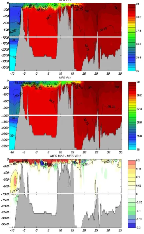
Fig. 4. Salinity cross section along the track shown in Fig. 1.
Bot-tom panel: difference between MFS V2.2 and MFS V2.1. The fields are the yearly mean for 2007.
In Fig. 3 the surface mean heat and water surface fluxes over the Mediterranean region are shown. The time series of the two simulations almost overlap, indicating that the sur-face fluxes over the Mediterranean region are not influenced by lateral boundary condition parameterizations in the At-lantic. Moreover, the estimated surface fluxes (Fig. 3), are in good agreement with analysed climatological values, as de-duced from NCEP 40 years re-analysis (Kistler et al., 2001). The only remarkable difference between simulated and ob-served values regards the amplitude of the seasonal cycle and we argue that this is due to the different length of the time-series used to compute climatologies (4 years for MFS and 40 years for NCEP).
Salinity vertical fields along the section crossing the whole Mediterranean Sea (red line in Fig. 1) are shown in Fig. 4
Fig. 5. Top panel: Time series of Mediterranean Sea mean surface
elevation from MFS V2.1 (solid line) and MFS V2.2 (dashed line) simulations. Bottom panel: Time series of mean surface elevation along the open boundaries from global model.
for both models together with their differences (Fig. 4 bot-tom panel); the fields shown are the 2007 yearly mean. In both model solutions the inflowing Atlantic water layer is ev-ident between 6◦W and 18◦E. Moreover, in agreement with the previous analyses, MFS V2.2 has higher Atlantic wa-ter salinity values at the surface. The increased salt content of the incoming Atlantic waters is not sufficient to strongly modify the stability of the water column. In the Atlantic side, the vertical stability is ensured by the combination of the large temperature gradient, the effect of the pressure and the salty Mediterranean outflow. In the Mediterranean Sea, where vertical gradients of temperature are less pro-nounced, the saltier Atlantic waters simulated by MFS V2.2 are still fresh enough to be buoyant. In the Western Mediter-ranean Sea some negative difference areas are observed be-low the intruding Atlantic waters, indicating that MFS V2.2 has patches of lower salinity than MFS V2.1. This is due to the different eddy dynamics in the area of the Algerian cur-rent, which results in a displacement of the eddies and jets. It is also interesting to note that the Mediterranean outflow in MFS V2.2 is saltier than in MFS V2.1.
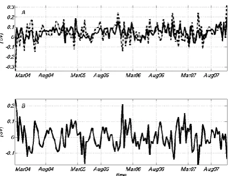
Fig. 6. (A) time-series of net volume transport at Gibraltar
Strait, solid line indicate MFS V2.1 results, dashed line indicates MFS V2.2 results. (B) time-series differences of net volume trans-port at Gibraltar between the two model simulations.
and the multiyear averaged Mediterranean sea level is about
−18 cm.
The global model sea level averaged along the lateral open boundaries (Fig. 5, bottom panel) shows a seasonal oscilla-tion of about 3cm connected to the Atlantic open ocean wind response. The minima in the North Atlantic mean surface elevation coincide with the Mediterranean yearly absolute minima (March), while some of the yearly maxima of the At-lantic and Mediterranean time series occur at different times. The mean surface elevation changes are driven by surface fluxes and the Gibraltar inflow. Taking the Mediterranean area average of Eq. (1) we obtain the time evolution equation for the surface average sea level,hηi:
∂hηi
∂t =
Gib
Amed
−
E−P − R
FR
. (4)
Where Gib is the net transport at Gibraltar (m3/s),Amedis the area of the Mediterranean Sea, and the 2nd term in the r.h.s. of the Eq. (4) is the Mediterranean average surface ter flux. As shown in Fig. 3, the area average surface wa-ter flux does not differ between MFS V2.1 and MFS V2.2, thus the differences in mean sea level oscillations, shown in Fig. 5, are due to the transport at Gibraltar. In particular, as-suming steady state in Eq. (4) the net transport value for Gib is 0.05 Sv, consistent with recent observations and calcula-tions (Menemenlis et al., 2007).
In Fig. 6a the time series of net mass transport through the Gibraltar Strait is shown. Both MFS V2.1 and MFS V2.2 time series have a time mean average of 4×10⁻²Sv but MFS V2.2 is characterized by larger oscillations. The differ-ences between the two simulations (Fig. 6b) have a seasonal cycle, with marked inter-annual variability, and the values can be as large as the average net transport. MFS V2.1 has
larger transport during early winter (January, February) and summer (August, September) while MFS V2.1 has smaller transport in spring (April, May) and fall (October). We can conclude that the differences induced in the Atlantic box produce different net transports at Gibraltar, which in turn induce mean sea level variations at the seasonal and inter-annual time scales. These fluctuations are clearly removed in the closed Atlantic box model case.
In order to understand whether the Atlantic influence on the Mediterranean Sea water mass structure and sea level is a real improvement, we will compare the two simulations with observations.
4 Quality assessment of the simulations
In this section we compare the simulations with observations deriving from ARGO floats (Poulain et al., 2007), satellite and tide gauge sea level.
The evaluation is done by means of standard statistics in-dexes such as Root-Mean-Square-Error (RMSE), Mean Er-ror (ME) and pattern correlation coefficient (PCC), and the comparison is presented in terms of a Relative Performance (RP) index. The RP has been defined as:
RP =
1−STV2.2
STV2.1
∗100 (5)
whereSTV2indicates the computed statistics (RMSE, ME or PCC) of MFS V2.1 and MFS V2.2. The PCC has been com-puted on the anomalies, subtracting the corresponding clima-tological mean profile for each dataset. The PCC has been also computed subtracting the same climatological profiles from both observations and model results (not shown), the results obtained with this method are very similar to the one presented in the following section. RP values>0 in Eq. (5) indicate an improvement (MFS V2.2 better than MFS V2.1) while RP values<0 show a deterioration. For PCC, the ratio of MFS V2.1 and MFS V2.2 is inverted in Eq. (5) in order to maintain the same interpretation of the index values. For instance, RP=50% means that the model error (RMSE, ME or PCC) has been reduced to half of its reference value, while RP=−100% indicates that the error in the MFS V2.2 is dou-ble respect to MFS V2.1. All the statistics considered have been averaged horizontally and temporally.
4.1 The temperature and salinity water mass properties
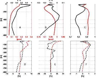
In Fig. 7a, b, c salinity and temperature RMSE, ME and PCC are shown for differences between ARGO profiles (shown in Fig. 1) and MFS V2.2.
Fig. 7. Upper panels: Temperature and Salinity RMSE (A), ME (B) and pattern correlation coefficient (C) vertical profiles for MFS V2.1.
Bottom panels: RP vertical profiles for RMSE (D) ME (E) and pattern correlation coefficient (F). Black lines indicate Temperature, red lines indicate salinity data.
salinity ME (Fig. 7b) are both negative indicating that the model underestimates salinity and heat content; moreover, the two curves have different shapes. In fact, the salinity ME has a sub-surface maximum located at 100 m depth, while temperature biases are larger near the bottom. Both tem-perature and salinity have high PCC values ranging between 0.75 and 0.95; moreover, temperature PCC has a minimum at 400 m depth, while salinity has it at 80 m depth. Results for MFS V2.1 are compared in terms of RP (bottom panels in Fig. 7) for each of the considered statistics. The temperature and salinity RP for RMSE are both positive, indicating that MFS V2.2 has greater skill than MFS V2.1. Moreover, the improvements in RMSE deriving from MFS V2.2 are mostly confined at the surface both for temperature (Fig. 7d dark line) and salinity (Fig. 7d, red line). The largest improve-ment is observed for salinity with RP values between 8 and 9%, while for temperature they are less than 5%, and a de-terioration of the solution is observed below 600 m depth, even if small (less than 2%). The most relevant differences between MFS V2.1 and MFS V2.2 concern the salinity ME (Fig. 7e). The RP for ME also has maximum values at the surface and, in this case too, MFS V2.2 seems to
repre-sent the salinity and temperature of the surface water bet-ter (dashed line RP>50% for salinity and RP>20% for tem-perature). A worsening of temperature ME is observed be-tween 100 and 200 m depth, with values close to 20% but, at these depths, both the model configurations have a small bias value, close to−0.05◦C.
The differences in PCC (Fig. 7f) are smaller than the other considered statistics, but for this indicator too MFS V2.2 has a greater skill for both temperature and salinity, with a max-imum between 100 and 200 m depth indicating an improve-ment in the reproduction of the mixed layer depth. Since PCC is an indicator of model performance in reproducing mesoscale activities, the small differences between the two simulations can be due to the fact the small scale features are locally formed and do not depend on the lateral boundary condition parameterization.
The slight deterioration of the MFS V2.2 solutions in the deeper layer could be related to the vertical mixing param-eterization, which maybe requires further tuning, having a better reproduction of the water masses characteristics.
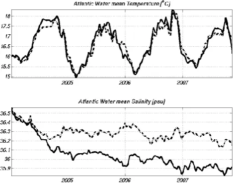
Fig. 8. Top panel: Time series of inflowing Atlantic water averaged
Temperature from MFS V2.1 (solid line) and MFS V2.2 (dashed line). Bottom panel: Time series of inflowing Atlantic water aver-aged Salinity from MFS V2.1 (solid line) and MFS V2.2 (dashed line).
Gibraltar Strait are shown. The mean temperatures (Fig. 8a) of the Atlantic water are very similar, with a clear and strong seasonal cycle. This is due to the fact that the Atlantic wa-ters entering into the Mediterranean Sea are surface wawa-ters and the air-sea fluxes totally determine their temperature. However the amount of the inflowing Atlantic water is dif-ferent between the two simulations (Fig. 6), thus the water masses can be differently advected producing the small dif-ferences in temperature observed within the Mediterranean Sea (Fig. 7).
On the contrary, the entering water has very different salt content in the two simulations (Fig. 8b). In the closed domain simulation the mean salinity of the Atlantic water decreases with time while in MFS V2.2 after the first year of integra-tion its values remain about constant with seasonal modu-lations. This is due to the fact the water (and salinity) sur-face fluxes in the two model implementations are different, in the Atlantic area, by the volume preserving correction fac-tor. The correction factor performed to preserve the volume in the closed simulation produces on average a dilution of the surface Atlantic waters.
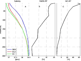
In order to have an estimate of the quality of the simu-lated Atlantic waters salinity, we compare model results with various ARGO buoys extracted, on the base of geographic location and surface salinity, from the entire data-set (green dots in Fig. 1). The intent of this sub-sampling is to filter out other water masses in the observations. A sub-sampling based only on the geographic locations was not sufficient due to the very complex Alboran Sea surface circulation with a number of gyres, eddies and jet. In Fig. 9 mean salinity pro-files from observations and models are shown together with the corresponding RMSE and ME RP indexes.
Both models underestimate surface salinity (from 0 to 300 m depth), but the MFS V2.2 configuration has strongly reduced this bias, especially in the first 30 m of the water column. The RP for RMSE at the surface is larger than 20% and it decreases going downward; below 150 m depth a wors-ening of the solution is observed but at this depth the models errors are very small (0.02 psu). Larger improvements, deriv-ing from the MFS V2.2 model configuration, are observed in the salinity ME. RP values at surface are close to 60% indicating that the bias, from MFS V2.1 to MFS V2.2, has halved.
In synthesis, MFS V2.2 generally captures better the salinity of the inflowing Atlantic water. We believe this is due to the freshening effect of the water flux volume preserving corrections discussed in Sect. 2 required by the closed model domain in the Atlantic. This behaviour was alleviated in the previous operational model implementation (MFS V1) since the water fluxE−P−R
FR
was computed relaxing to sur-face climatological salinity.
4.2 Surface elevation seasonal oscillation
In this section we would like to show that the Mediterranean seasonal mean sea level oscillations from MFS V2.2, shown in Fig. 5, compare better with observations than MFS V2.1. To do this, we compare the model simulated sea surface el-evations with the corresponding field obtained from altime-try sea level and tide gauges. The altimeter products (Sea Level Anomaly, SLA) were produced by Ssalto/Duacs and distributed by Aviso, with support from CNES; in particular we used Envisat and Jason-1 along-track satellite sea level anomaly data (see Pujol and Larnicol, 2005, for details). The tide gauge data have been provided by the Italian Agency for Environmental Protection.
Following Mellor and Ezer (1995) and Greatbatch (1994), sea level in a Boussinesq, incompressible, model like ours needs to have the steric effect added before it can be com-pared with observations. The importance of the steric effect in the observed record is discussed in Cazenave et al. (1998). In order to take into account the non-Boussinesq effects in our model results, vertical and horizontal means of the model density profiles have been computed for each day of the sim-ulations and added to the model sea level. Mellor and Ezer (1995) show that this is enough to restore the full sea level variability of a non-Boussinesq model.
Fig. 9. (A) vertical profiles of salinity, obtained averaging observations and model data in the green dots shown in Fig. 1. Blue line indicates
observations (ARGO floats), green line indicate MFS V2.1 results and red line indicates MFS V2.2 results. Relative performance index for salinity for RMSE (B) and mean-error (C).
It is clear that MFS V2.2 better reproduces the ampli-tude and the shape of the observed seasonal cycle, while MFS V2.1 strongly underestimates the observed seasonal variability.
One of the most interesting features captured by the in-teraction with the Atlantic in the MFS V2.2 model is the summer-autumn maxima. In fact, both the satellite and model (MFS V2.2) time series are characterized by dou-ble maxima; the first occurring in August and the sec-ond in November–December. Some differences between MFS V2.1 solution and satellite-derived observations are still present, and are mostly due to the correct reproduction of the inter-annual variability. The summer maximum, as discussed before, is also observed in the global model so-lution; we thus argue that this large scale induced processes. The other maxima are due to local (Mediterranean) processes that in the nested simulation are free to develop while in the closed simulation are suppressed.
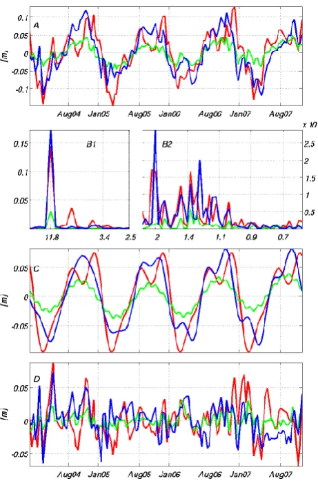
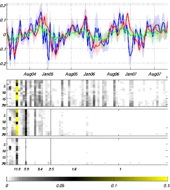
In order to better understand the differences and similar-ities between simulated and observed surface elevation, the power spectrum of the three time-series is shown in Fig. 10b. For all the considered datasets the spectrum is discontinu-ous and characterized by well marked maxima. In the satel-lite observations 42% of the total variance (0.45 m2) is ex-plained by the first 3 dominant frequencies corresponding at 12, 4 and 6 months−1 and having energies of 0.17 (38%), 0.011 (2.5%) and 0.004 m2(0.8%) respectively. MFS V2.2
has comparable energy content (0.49 m2) but distributed in a different way: the 12-month−1oscillation energy is about 0.14 m2(corresponding to 30% of the total); the energy as-sociated with the 6-month−1frequency is 0.035 m2(7%) and the 4-month−1 frequency has 0.014 m2 associated energy (2.8%). The total variance in the MFS V2.1 simulation is 0.08 m2, significantly smaller than the observed value; 37% (0.03 m2) of this variance is due to an oscillation with fre-quency of 12 months−1; the residual part is distributed ho-mogeneously in the remaining frequencies.
In addition, it is interesting to note that at higher frequen-cies (Fig. 10b2), satellite and MFS V2.2 power spectra are similar (MFS V2.2 has the right variance at the right frequen-cies), while MFS V2.1 also underestimates the amplitude of the signal at these scales.
Fig. 10. (A) Time series of Mediterranean Sea mean surface
el-evation from MFS V2.1, MFS V2.2 simulations and satellite ob-servation. The steric effect has been superimposed on the model results. (B) Power spectrum for observed (blue line) and modelled (MFS V2.1 green, MFS V2.2 red line) surface elevation. (C) Time series of Mediterranean Sea mean surface elevation reconstructed using only the first three dominant frequencies in the power spec-trum. (D) Time series of Mediterranean Sea mean surface elevation reconstructed using all the frequencies removed from panel (C).
and data can be attributed here to the use of climatological monthly fields for the nesting in the Atlantic.
MFS V2.1 fails both in reproducing the double summer-autumn and the local maxima occurring in February. It is also clear that MFS V2.1 underestimates the energy content in the remaining part of the frequency spectrum (Fig. 10d).
As further evaluation of the surface elevation, model re-sults have been compared with available tide gauges (cyan dots in Fig. 1) data; observations have been averaged in time in order to remove tidal signal, model results have been sam-pled on the tide gauges positions. In this case too the steric effect has been superimposed to the model results.
The time series of the surface elevation, averaging all the available tide gauge station data from MFS V2.1, MFS V2.2
simulations and tide gauge observations are shown in Fig. 11. Major differences with satellite-derived surface elevation concern the annual minima that in the tide gauge time se-ries occur in January. Both the model implementations fail in reproducing this feature. Due to the absence of this mini-mum in the satellite observations, we argue that this is prob-ably due to coastal processes not resolved with our model resolution. In this case too the MFS V2.2 reproduces the amplitude of the seasonal signal and the occurrence of the double summer-autumn maxima better; this model configu-ration is also able to reproduce the less pronounced observed autumn maxima in 2007. Power spectra (Fig. 11 bottom pan-els) confirm that MFS V2.2 is able to reproduce the energy content of the dominant frequencies (12, 6 and 4 months−1), while MFS V2.1 fails in simulating the 6- and 4-month os-cillations. Differently from the satellite data, the tide gauge surface elevations also show a significant energy content at higher frequency (higher than 2.5 months−1).
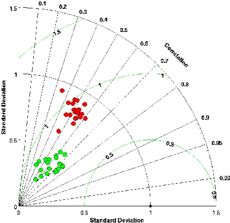
Figure 12 is a Taylor diagram (Taylor, 2001) which sum-marizes the relative skill with which MFS V2.1 (green cir-cles) and MFS V2.2 (red circir-cles) implementations simu-late the temporal evolution of surface elevation recorded by the tide gauges. MFS V2.2 correlation with observa-tions is about 0.5; the standard deviation of the simulated field is slightly smaller than the observed standard deviation. MFS V2.1 has a slightly higher correlation (0.6) with ob-servations but strongly underestimated the amplitude of the variations, with a normalized standard deviation of about 0.3. The lower correlation with the observation of MFS V2.2 is due to the high frequency oscillations that in some cases are delayed with respect to the observations (Fig. 11 upper panel), producing higher error.
5 Summary and conclusion
Fig. 11. Top panel: Time series of mean surface elevation from MFS V2.1 (green line), MFS V2.2 (red line) simulations and tide gauge
observations (blue line). The steric effect has been superimposed on the model results. The shaded coloured areas show the two standard deviation ranges. Bottom panels: Power spectra for observed and modelled surface elevation (from top to bottom: observation, MFS V2.2 and MFS V2.1). X-axis indicate station number; Y axis indicate frequency in month−1, colour indicate the energy in m2.
al. (2008); the model has three closed boundaries in the At-lantic (Fig. 1) where active tracers (temperature and salinity) are relaxed toward monthly climatological data; as a conse-quence of the closed-domain approach the mass is preserved using a correction factor in the Atlantic area that compen-sates the surface mass flux occurring in the Mediterranean. MFS V2.2 has three open boundaries in the Atlantic where it is nested with the same monthly climatological fields used for the relaxation in the MFS V2.1 version; as a consequence of the dynamical nesting, no particular correction needs to be applied to the surface forcing functions.
As a first guess the model is able to reproduce the Mediter-ranean observed dynamics with a skill comparable to previ-ous model efforts in the Mediterranean Sea (Fig. 7). Ma-jor differences between the two simulations result concern-ing the proprieties of the inflowconcern-ing Atlantic water (Fig. 8) and a seasonal variation of the Mediterranean water volume (Fig. 5).
In the closed domain implementation, a freshening of the inflowing Atlantic water proprieties has been observed (Fig. 8); this deterioration (Fig. 9) is due to the necessity of preserving the volume in the whole domain. As the Mediter-ranean Sea is a concentration basin, the correction factor ap-plied in the Atlantic area is, in general, positive (water from the atmosphere into the ocean) with the obvious consequence of diluting the surface Atlantic waters. In order to overcome this problem alternative solutions have been adopted in the past, but in all the considered cases they represent compro-mises between physical coherent (realistic) representation of the surface processes and suitability of the numerical solu-tion.
Fig. 12. Model implementation vs. tide gauge observation Taylor
diagrams. Red circles indicate MFS V2.2, green circles indicate MFS V2.1.
This is equivalent to supposing that precipitation has same salinity as surface Atlantic water. Major disadvantage of this approach are: low reliability of surface fluxes for both vertical component of the momentum and salinity; this flux does not take into account real air-sea exchanges but only a difference with corresponding climatological values; sur-face boundaries for vertical velocity and salinity are not re-lated each other (Beron-Vera et al., 1999) in the Atlantic area. This is clearly non-consistent but allows a reasonable solu-tion within the Mediterranean Sea insofar as regards surface salinity values, and it is particularly suitable for operational purposes.
In the MFS V2.1 (closed implementation) discussed in this work we used coherent surface boundary condition for vertical velocity and salinity; this approach gave us the pos-sibility to have realistic surface fluxes over the Mediterranean Sea (Fig. 3) but at the same time it also causes the freshening of the Atlantic waters. On the contrary, in MFS V2.2, using a nesting approach, the volume conservation issue is managed by the lateral boundary condition parameterization and there is no need to apply a correction factor to the surface fluxes; this allows a better representation of the inflowing Atlantic water proprieties (Figs. 8 and 9).
One of the major findings deriving from the nesting ap-proach concerns a large scale seasonal oscillation of the Mediterranean volume (Fig. 5). The adopted lateral bound-ary condition allows the volume of the domain to vbound-ary ac-cording to the transport imposed by the nesting model and, at the same time, on the base of equilibrium between nested and nesting models continuity equations (4). Seasonal
varia-tion of Mediterranean volume in the MFS V2.1 implementa-tion are due mostly to steric effect, while in MFS V2.2 and in the observed datasets the steric effect seasonal cycle is mod-ulated by oscillations with similar frequencies (Fig. 10a). As a consequence the amplitude of the 12-month period oscilla-tion in MFS V2.1 is underestimated.
In particular, the summer maximum observed in both the satellite data and tide gauges is reproduced by the model us-ing the nestus-ing approach (Fig. 10a and c). The dominant fre-quency in all the considered dataset (satellite, tide gauges and both model implementations) is about 12 months−1; more-over, observations and MFS V2.2 results are then modu-lated by oscillation with frequencies ranging between 3.5 and 6 months−1.
Compared with satellite-derived data, in the open-domain simulation there is also the correct amount of energy at higher frequencies (ranging between 1 and 2 months−1), while MFS V2.1 strongly underestimates this part of the signal (Fig. 10b2). This is probably due to the fact that with a nesting approach the model has a greater degree of freedom and a larger number of oscillations are allowed. Dictated by operational needs, the future development will be to nest the model with high-frequency inter-annual fields from the MERCATOR operational system. A better temporal resolution of the nesting model should allow a more realistic reproduction of inter-annual variability in the Mediterranean Sea.
Edited by: M. Hecht
References
B´eranger, K., Mortier, L., and Cr´epon, M.: Seasonal variability of water transports through the Straits of Gibraltar, Sicily and Cor-sica, derived from a high resolution model of the Mediterranean circulation, Progress in Oceanography, 66(2–4), 341–364, 2005. Beron-Vera, F. J., Ochoa, J., and Ripa, P.: A note on boundary con-ditions for salt and freshwater balances, Ocean Model., 1, 111– 118, 1999.
Bozec, A., Bouruet-Aubertot, P., B´eranger, K., and Cr´epon, M.: Mediterranean oceanic response to the interannual vari-ability of a high-resolution atmospheric forcing: A fo-cus on the Aegean Sea, J. Geophys. Res., 111, C11013, doi:10.1029/2005JC003427, 2006.
Cazenave, A., Dominh, K., Gennero, M. C., and Ferret, B.: Global mean sea level changes observed by Topex-Poseidon altimetry and ERS-1, Phys. Chem. Earth, 23, 1069–1075, 1998.
Demirov, E. and Pinardi, N.: The simulation of the Mediterranean Sea circulation from 1979 to 1993. Part I: The interannual vari-ability, J. Mar. Syst., 33–34, 23–50, 2002.
Drevillon, M., Bourdall´e-Badie, R., Derval, C., Drillet, Y., Lel-louche, J. M., R´emy, E., Tranchant, B., Benkiran, M., Greiner, E., Guinehut, S., Verbrugge, N., Garric, G., Testut, C. E., La-borie, M., Nouel, L., Bahurel, P., Bricaud, C., Crosnier, L., Dombrosky, E., Durand, E., Ferry, N., Hernandez, F., Le Gal-loudec, O., Messal, F., and Parent, L.: The GODAE/Mercator-Ocean global ocean forecasting system: results, applications and prospects, J. Operational Oceanogr., 1(1), 51–57, 2008. Estubier, A. and L´evy, M.: Quel sch´ema num´erique pour le
transport d’organismes biologiques par la circulation oc´eanique, Note Techniquesdu Pˆole de mod´elisation, Institut Pierre-Simon Laplace, 81 pp, 2000.
Fekete, B. M., V¨or¨osmarty, C. J., and Grabs, W.: Global, Compos-ite Runoff Fields Based on Observed River Discharge and Simu-lated Water Balances, Tech. Rep. 22, Global Runoff Data Cent., Koblenz, Germany, 1999.
Flather, R. A.: A tidal model of the northwest European continen-tal shelf, Memories de la Societe Royale des Sciences de Liege, 6(10), 141–164, 1976.
Fukumori, I., Menemenlis, D., and Lee, T.: A near-uniform basin-wide sea level fluctuation of the Mediterranean Sea, J. Phys. Oceanogr., 37, 338–358, 2008..
Greatbatch, R. J.: A note on the representation of steric sea level in models that conserve volume rather than mass, J. Geophys. Res., 99(C6), 12767–12771, 1994.
Kistler, R., Kalnay, E., Collins, W., Saha, S., White, G., Woollen, J., Chelliah, M., Ebisuzaki, W., Kanamitsu, M., Kousky, V., Van den Dool, H., Jenne, R., and Fiorino, M.: The NCEP-NCAR 50-Year Reanalysis: Monthly Means CD-ROM and Documentation, B. Am. Meteorol. Soc., 82, 247–268, 2001.
Kondo, J.: Air-sea bulk transfer coefficients in diabatic conditions, Bound.-Lay. Meteorol., 9, 91–112, 1975.
Kourafalou, V. H. and Barbopoulos, K.: High resolution simula-tions on the North Aegean Sea seasonal circulation, Ann. Geo-phys., 21, 251–265, 2003,
http://www.ann-geophys.net/21/251/2003/.
Lascaratos, A., Williams, R. G., and Tragou, E.: A mixedlayer study of the formation of Levantine intermediate water, J. Geo-phys. Res., 98, 14739–14749, 1993.
Levitus, S.: NODC World Ocean Atlas 1998 data, report: NOAA-CIRES Clim. Diag. Cent. Boulder, Colorado, 1998.
L´evy, M., Estublier, A., and Adec, G.: Choice of an advection scheme for biogeochemical models, Geophys. Res. Lett., 28(19), 3725–3728, 2001.
Madec, G., Delecluse, P., Imbard, M., and Levy, C.: OPA8.1 Ocean general Circulation Model reference manual. Note du Pole de modelisazion, Institut Pierre-Simon Laplace (IPSL), France, 11, 1998.
Madec, G.: NEMO ocean engine, Note du Pole de mod´elisation, Institut Pierre-Simon Laplace (IPSL), France, No 27 ISSN No 1288-1619, 2008.
Marchesiello, P., McWilliams, J. C., and Shchepetkin, A.: Open boundary conditions for long term integration of regional oceanic models, Ocean Model., 3, 1–20, 2001.
Mariotti, A., Struglia, M. V., Zeng, N., and Lau, K. M.: The Hy-drological Cycle in the Mediterranean Region and Implications for theWater Budget of the Mediterranean Sea., J. Climate, 15, 1674–1690, 2002.
Mellor, G. L. and Ezer, T.: Sea level variations induced by heating
and cooling: An evaluation of the Boussinesq approximation in ocean models, J. Geophys. Res., 100(C10), 20565–20577, 1995. Menemenlis, D., Fukumori, I., and Lee, T.: Atlantic to Mediter-ranean sea level difference driven by winds near Gibraltar Strait, J. Phys. Oceanogr., 37, 359–376, 2007.
Oddo, P. and Pinardi, N.: Lateral open boundary conditions for nested limited area models: A scale selective approach, Ocean Model., 20, 134–156, 2008.
Orlanski, I.: A simple boundary condition for unbounded hyper-bolic flows, J. Comput. Phys., 21, 251–269, 1976.
Pinardi, N. and Flemming, N. C.: The Mediterranean Forecasting System Science Plan, EuroGOOS Publication no. 11, Southamp-ton Oceanography Centre, 48 pp., ISBN 0-904175-35-9, 1998. Pinardi, N., Allen, I., Demirov, E., De Mey, P., Korres, G.,
Las-caratos, A., Le Traon, P.-Y., Maillard, C., Manzella, G., and Tziavos, C.: The Mediterranean ocean forecasting system: first phase of implementation (1998–2001), Ann. Geophys., 21, 3–20, 2003,
http://www.ann-geophys.net/21/3/2003/.
Pinardi, N., Arneri, E., Crise, A., Ravaioli, M., and Zavatarelli, M.: The physical, sedimentary and ecological structure and variabil-ity of shelf areas in the Mediterranean Sea, The Sea, vol. 14, edited by: Robinson, A. R. and Brink, K., Harvard University Press, Cambridge, USA 1243-1330, 2006.
Poulain, P.-M., Barbanti, R., Font, J., Cruzado, A., Millot, C., Gert-man, I., Griffa, A., Molcard, A., Rupolo, V., Le Bras, S., and Petit de la Villeon, L.: MedArgo: a drifting profiler program in the Mediterranean Sea, Ocean Sci., 3, 379–395, 2007,
http://www.ocean-sci.net/3/379/2007/.
Pujol, M. I. and Larnicol, G.: Mediterranean Sea eddy kinetic en-ergy variability from 11 years of altimetric data, J. Mar. Syst., 58(3–4), 121–142, 2005.
Raicich, F.: On fresh water balance of the Adriatic Sea, J. Mar. Syst., 9, 305–319, 1996.
Robinson, A. R. and Golnaraghi, M.: The physical and dynami-cal oceanography of the Mediterranean Sea, in: Ocean Process-esin ClimateD ynamics: Global and MediterraneanE xamples, edited by: Malanotte-Rizzoli, P. and Robinson, A. R., pp. 255– 306, Kluwer Acad., Norwell, Mass., 1994.
Roussenov, V., Stanev, E., Artale, V., and Pinardi, N.: A seasonal model of the Mediterranean Sea general circulation, J. Geophys. Res., 100(C7), 13515–13538, 1995.
Taylor, K. E.: Summarizing multiple aspects of model performance in a single diagram, J. Geophys. Res., 106, 7183–7192, 2001. Testor, P., B´eranger, K., and Mortier, L.: Modeling the deep
eddy field in the southwestern Mediterranean: the life cy-cle of Sardinian Eddies, Geophys. Res. Lett., 32(13), L13602, doi:10.1029/2004GL022283, 2005..
Tonani, M., Pinardi, N., Dobricic, S., Pujol, I., and Fratianni, C.: A high-resolution free-surface model of the Mediterranean Sea, Ocean Sci., 4, 1–14, 2008,
http://www.ocean-sci.net/4/1/2008/.
Van Leer, B.: Towards the Ultimate Conservative Difference Scheme, V. A Second Order Sequel to Godunov’s Method, J. Comput. Phys., 32, 101–136, 1979.