Article Compulsory Schooling and Returns to Education: A Re-Examination

econometrics

Article

Compulsory Schooling and Returns to Education:

A Re-Examination

Sophie van Huellen * and Duo Qin

SOAS University of London, Thornhaugh Street, Russell Square, London WC1H 0XG, UK

* Correspondence: [email protected]; Tel.:+44-(0)-20-7898-4543

Received: 25 May 2019; Accepted: 29 August 2019; Published: 2 September 2019

Abstract:This paper re-examines the instrumental variable (IV) approach to estimating returns to education by use of compulsory school law (CSL) in the US. We show that the IV-approach amounts to a change in model specification by changing the causal status of the variable of interest. From this perspective, the IV-OLS (ordinary least square) choice becomes a model selection issue between non-nested models and is hence testable using cross validation methods. It also enables us to unravel several logic flaws in the conceptualisation of IV-based models. Using the causal chain model specification approach, we overcome these flaws by carefully distinguishing returns to education from the treatment effect of CSL. We find relatively robust estimates for the first effect, while estimates for the second effect are hindered by measurement errors in the CSL indicators. We find reassurance of our approach from fundamental theories in statistical learning.

Keywords: instrumental variables; randomisation; research design; average return to education

JEL Classification:C26; C52; I21; I26; J24

1. Introduction

Over the past century, compulsory school law (CSL) was introduced in virtually every middle and high-income country (Goldin 1998;Goldin and Katz 2007). Empirical investigations into the effect of the CSL on educational attainment and income were pioneered byAngrist and Krueger(1991). The authors used CSL indicators as instrumental variables (Ivs) to ‘randomise’ latent ability across educational attainment groups to correct for the presumed inconsistency or beyond-sample bias in the ordinary least square (OLS) estimator. The empirical strategy is now common practice in research on the average return to education (ARTE) and the paper has since entered the standard economics curriculum, as evident from its appearance in two popular textbooks byAngrist and Pischke(2009,2015).

Despite the far-reaching influence of this strategy, the causal interpretation of the CSL-treated schooling coefficient remains contentious. This is reflected in two interlinked developments. First, the emergence of IV estimates that vary significantly with the choice of instruments. Angrist and Krueger(1991), who approximate CSL with quarter of birth dummies, find that the IV estimates are not statistically different from estimates obtained via OLS.1_{Acemoglu and Angrist(2001) andStephens and} Yang(2014) replicate the research design byAngrist and Krueger(1991) with alternative CSL indicators based on labour law and find IV estimates which, although significantly different from OLS estimates, are insignificant or negative.2 Second, a shift in the interpretation of the CSL instrumentalised returns

1 _{E.g., column (5) versus (6) in Table 4, (7) versus (8) in Table 5, and (1) versus (2) and (5) versus (6) in Table 6 inAngrist and}

Krueger(1991).Hoogerheide and van Dijk(2006, Table 5) and inHarmon et al.(2003, sec. 5).

2 _{SeeAngrist and Pischke(2015, Table 6.3) for a summary.}

Econometrics2019,7, 36 2 of 20

to schooling coefficient despite identical model choice. Angrist and Krueger(1991) interpret their results as consistent estimates of the ARTE, whereasStephens and Yang(Stephens and Yang 2014, p. 1789) interpret their IV estimates as the effect of an additional year of education obtained due to CSL on income.

The first development prompts the question of how to select one consistent IV estimate among a multitude of IV choices. The second development prompts questions over the causal meaning of the IV estimates. The literature has responded to these questions by declaring certain instruments as inadequate, e.g., seeAngrist and Pischke(2015, p. 227) for the above cases andStock et al.(2002) andKolesár et al.(2015) more generally, and by pointing at sample heterogeneity in the CSL effect, seeStephens and Yang(2014),Angrist et al. (1996), andAngrist and Imbens(1995) more generally.3 However, the credibility of this empirical strategy is still disputed methodologically; seeDeaton(2009) andDeaton and Cartwright(2018).

In this paper, we approach and analyse the contention from a different perspective. Drawing on fundamental concepts and theories from statistical learning, we argue that what is commonly described as a choice of consistent estimator is a choice of causal model design, whereby model choice has far more substantial implications for the consistency criterion than estimator choice. Further, a change in causal model design implies a change in the key causal variable, leading to a change in causal meaning of coefficient estimates. From this perspective, we can provide clarification regarding the questions raised and hopefully settle the methodological dispute. We demonstrate our arguments by replication and re-examination of two seminal studies byAngrist and Krueger(1991) (AK hereafter) andStephens and Yang(2014) (SY hereafter).4

The insights gained from this new perspective are a consequence of two observations. First, the essence of the IV approach is the modification of a presumed endogenous causal variable, whereby the causal variable is substituted by regressors produced from non-uniquely and non-causally specified, and non-optimally targeted regressions; seeQin(2015,2018) for a more detailed methodological exposition. Empirical evaluation and selection of these generated regressors is hence a source of endless contention. Second, the theoretical proof of IV estimator consistency rests on the presumption that the associated model specification is globally valid. This presumption is unlikely to hold in practice, as revealed by the out-of-sample error decomposition, known as the bias-variance tradeoff in the statistical learning literature. Analysis of this decomposition points to model bias rather than estimator bias as the primary source of inferential bias. Further, the presumption rules out any form of empirical model selection, including the choice between different instruments. This presumption is hence in conflict with the practical application of the IV approach.

Approaching the issue of modelling ARTE from this new perspective in Section2, we show that the use of IV estimators amounts to making, albeit implicitly, the presumption of the education variable being an invalid conditional variable, thereby changing the causal model specification. Conceptualising the choice of the IV versus the OLS as one of causal model choice between non-nested model alternatives, this presumption can be explicitly specified into testable hypotheses. Moreover, the conceptualisation reveals the need to clarify the causal role of the CSL instruments. The causal chain representation method byCox and Wermuth(2004) is applied to unravel the shift in interpretation of causal parameter estimates. While promiscuous in the IV approach, the chain representation makes possible the clear separation of two types of income effects: The ARTE with a possible moderation effect of CSL and the

3 _{This argument is related to the programme evaluation modelling literature where the treatment variable, a dummy, is}

endogenised; e.g.,Harmon et al.(2003) andLudwig et al.(2012,2013). The average treatment effect (ATE) estimate becomes a local ATE (LATE) estimate confined to the complier group if the instrument’s effect is heterogeneous, e.g., seeAngrist and Pischke(2009, chp. 4);Heckman and Urzua(2009);Deaton(2009); andImbens(2010). However, this discussion is virtually irrelevant here as the treatment variable, i.e., CSL, has not been considered as endogenous in either studies.

4 _{The two data sets used in these studies are both created from the 1980 US census but with different indicators and choice of}

Econometrics2019,7, 36 3 of 20

average treatment effect (ATE) of the CSL via schooling. The separation further enables us to assess risk of bias, i.e., omitted variable bias (OVB), measurement error, and selection bias, at the level of individual causal parameters.

In Section3, we find no evidence of convergence as a necessary condition for consistency of the IV models, regardless the choice of instruments by k-fold cross validation (CV). CV is an essential tool for out-of-sample comparison of model generalisability, stability, and consistency in statistical learning. Further, decomposition of the two income effects, ARTE and the ATE of CSL via schooling, in Section4reveals that firstly, relatively robust ARTE estimates across cohorts and data sets can be obtained when carefully choosing covariates. Secondly, the estimated ATE effects of CSL and the CSL moderation effects on schooling are undermined by considerable measurement-error problems in the CSL indicators provided in AK and SY. Specifically, by careful choice of covariates, we find a virtually invariant and empirically consistent ARTE estimate of 0.06, and a smaller ATE of the CSL estimates between 1–5% if using labour law indicators and 0.2–0.9% if using quarter of birth indicators. It should be noted, however, that the empirical analysis is limited by the available covariates and instruments provided by AK and SY.

The empirical results in Section4show us how a causally explicit model design through statistical data learning enables us to clearly separate, empirically and conceptually, the causal meaning of parameter estimates and to assess the risk of inferential bias at the level of individual parameters. Methodological implications of these findings are extended in Section5.Angrist and Pischke(2015, p. 227) discard theAcemoglu and Angrist(2001) study as ‘a failed research design’ and ascribe the failure to the choice of inappropriate CSL indicators. While we also find shortcomings in the CSL instruments, we delve deeper into the failure to reveal its root in equivocal causal model modifications by choosing the IV-based modelling approach. This choice virtually prevents direct and careful translation of causal postulates of interest into data-consistent conditional relationships. Although being constrained by the data sets provided in AK and SY, our re-examination of the CSL case clearly shows the importance of empirical model design and selection over estimator choice.

2. Model Specification of Schooling Effects Under CSL Treatment

The main objective of both AK and SY is to obtain consistent estimates of the effect of education on income, known as the ARTE. They reject, as inconsistent, the OLS in favour of the IV estimator. In contrast to previous literature, we transpose the OLS versus IV estimator choice into a choice of non-nested conditional models. This transposition leads us to re-evaluate the consistency claim underlying the choice of the IV approach and helps us to disentangle the seemingly conflicting causal interpretations presented in AK and SY. To facilitate the task, we adopt the subscript-based parametric notational methods used byCox and Wermuth(2004) to highlight the consequence of different causal specifications on the parameters of regressors.

Denote education bys, and income byy, the OLS-based approach of estimating ARTE amounts to proposing the following simple regression model:

y=αy+βyss+ηy (1)

(1) is perceived as an invalid conditional model by both AK and SY on the presumption that

cov(sη),0. The presumption is based mainly on the argument that (1) suffers from omitted variable bias (OVB), i.e.,ηycontains variables which are not directly observable but collinear withs, such as aptitude. Their remedy is to utilise the CSL as a key instrument to block this bias. Specifically, the following regression is used to generatesL_{, the fitted response from (2):}

s=πsL.IjL+I

0

jγsIj.L+es ⇒ s

L_{, (2)}

Econometrics2019,7, 36 4 of 20

y=αy+βysLsL+ηL_y. (3)

From the perspective of model specification, (1) and (3) are de facto non-nested models. The necessary condition for having statistically significantβys , βysL is to generatesL, such thatsLs.5 In general, since no unique set of Ivs exist for (2) in practice, it is impossible to settle a priori on one unanimously agreed definition ofsL.6 That implies that (3) should be seen as representing a multitude of non-nested models. Modellers are compelled to go through a model selection process, albeit implicitly through experimenting with various IV sets, as seen in both the AK and SY cases. One drawback of this implicit practice is the lack of model selection rules for guidance.

Once the task is recognised as one of model selection rather than estimator selection, out-of-sample cross validation (CV) methods, which are widely used in statistical learning, emerge as a useful toolbox to evaluate beyond-sample inferential bias. According to statistical learning theory, model selection is targeted at structural risk minimisation over a given hypothesis space that spans over the competing model specifications. A model is selected against its alternatives based on the interlinked criteria of generalisability (or predictivity), stability, and consistency, wherebyMukherjee et al. (2006) show that stability is equivalent to empirical consistency. CV methods are designed to assess predictivity and consistency by splitting the sample into k-folds, with k-1 folds being used to train the model and the kth fold to test the model. The competing model specifications can hence be evaluated by comparison of the relative mean squared error (MSE) in a k-fold CV, e.g., seeArlot and Celisse(2010), Shalev-Shwartz et al.(2010) andZhang and Yang(2015).7

At the core of CV methods is the analysis of MSE through its decomposition into bias and variance, and the demonstration of the tradeoffbetween the two components. In particular, the analysis identifies model bias as the primary source of inferential bias, i.e., the bias component in the out-of-sample or the testing sample errors. Another fundamental insight from statistical learning is the recognition that theoretical models, i.e., formal constructs of prior knowledge, are the source of inductive bias. Hence, in the quest for structural risk minimisation, major attention is paid to the minimisation of inductive bias in model selection and model design, see e.g.,Shalev-Shwartz and Ben-David(2014, Part I). In light of these fundamental theories, we see the need, in addition to the application of CV, of scrutinising carefully the process of how schooling effects on income under the CSL treatment are formalised into (3). Especially, whether the various contextual reasons supporting its formalisation, such as OVB and related measurement errors as well as selection bias, can justify the rejection of (1).

Since the CSL effect on income via schooling is a sequential event, this can be represented by a reduction of the following recursive factorisation of the joint density, f(y,s,L):

f(y,s,L) = f(y

s,L)f(s|L)f(L) = f(y

s,L)f(s|L), (4) since f(L) =1 when retrospective cross-section data samples are used. WhenLis assumed to act as a rule of intervention, namely y⊥_L

s, the conditional density in (4) can be further factorised: f(y,s

L) = f(y

s)f(s|L). (5)

On the basis of (5), we can express the sequential nature of the ATE ofLonyviasby the conditional expectation,E(y,s

L) =E(y

s)E(s|L). In a linear model setting, this expectation decomposition leads to the following chain model representation, seeCox and Wermuth(2004):

y=αy+βyss+ηy

s=αs+βsLL+ηs (6)

5 _{Notice that this requirement imposes a non-optimal prediction constraint on (2), in that the specification of this regression}

mustavoidexplaining the response variable as accurately as possible.

Econometrics2019,7, 36 5 of 20

It should be noted that (6) differs from (2)+(3) in two substantial ways. First,βysstill embodies ARTE in (6). Second, the ATE ofLony, denoted byβyL, is derivable fromβyL=βysβsL, whereas there lacks a clear parametric representation of this effect in the IV model. AlthoughπsL.Ij in (2) can be interpreted as the ATE ons, this parameter cannot be used in conjunction withβ_ysLin (3) to identify the ATE ony.

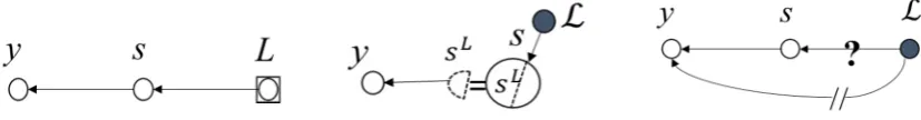
An arguably useful tool to highlight these differences is the directed acyclic graph (DAG), seeCox and Wermuth(1996) andWermuth and Cox(2011). The left panel of Figure1is a DAG of (6). It shows us that, when ATE, i.e., the effect ofLforms the focal causal interest,stakes the role of an intermediate variable or a mediator, but when ARTE is the focal interest,Ltakes the role of a moderator exclusively fors. The second arrow segment, L→_{s, can be ignored in the latter case, i.e., the case when (6) is} reduced into (1). The middle panel is a DAG of (2)+(3).8This IV-based model is focused on the first arrow segment, since its objective is to reject (1). Hence, the possibility of a causal chain extension is blocked, andLis used to target at producingsLs, making ATE ofLonyunidentifiable—but neither is ARTE identifiable becauseshas been significantly modified. Therefore, the definition ofβysLneeds to be modified.

Econometrics 2019, 7, x FOR PEER REVIEW 5 of 20

be interpreted as the ATE on s, this parameter cannot be used in conjunction with 𝛽 in (3) to identify the ATE on y.

An arguably useful tool to highlight these differences is the directed acyclic graph (DAG), see Cox and Wermuth (1996) and Wermuth and Cox (2011). The left panel of Figure 1 is a DAG of (6). It shows us that, when ATE, i.e., the effect of L forms the focal causal interest, s takes the role of an

intermediate variable or a mediator, but when ARTE is the focal interest, L takes the role of a

moderator exclusively for s. The second arrow segment, 𝐿 → 𝑠, can be ignored in the latter case, i.e., the case when (6) is reduced into (1). The middle panel is a DAG of (2) + (3).8 _{This IV-based model is}

focused on the first arrow segment, since its objective is to reject (1). Hence, the possibility of a causal chain extension is blocked, and L is used to target at producing 𝑠 ≉ 𝑠, making ATE of L on y

unidentifiable—but neither is ARTE identifiable because s has been significantly modified. Therefore, the definition of 𝛽 needs to be modified.

Figure 1. Directed acyclic graphs (DAGs) of returns to schooling under the compulsory school law (CSL) treatment. Notes: y denotes earnings; s, schooling; L, the CSL; and ℒ, its observable indicator. A node inside a square indicates a latent variable, and a solid node denotes a dummy/binary variable. Dotted lines indicate non-uniqueness; dissimilarity of 𝑠 from s is shown by a semicircle; the ‘identity’ sign differentiates the first stage of the 2SLS, (2).

Now, we are in the position of examining the contextual reasons underlying (3) to find out whether the IV-induced modification helps resolve the problems that the approach is intended. Although OVB is stated as the primary problem by AK, it is further compounded, in their justification for the IV route, with two problems—measurement error and selection bias. In view of the current

modelling purpose, the concern over measurement error in s is unwarranted because ARTE is not

ARTA (average returns to aptitude).9 _{In other words, measurement error is irrelevant in (1) unless}

we change its prior stance to explicitly specify s as an imperfect indicator of the latent variable,

‘aptitude’. However, measurement error can provide 𝛽 in (3) with a plausible interpretation

differently from that of 𝛽 . However, this interpretation would undermine the basic IV-based claim of 𝛽 being the consistent estimator of ARTE with respect to s, and openly recognise (1) and (3) as two different models, with (3) effectively yielding ARTA. As for selection bias, the argument extends to the situation where CSL treatment could alter the population composition of educated workers, as compared to that of the pre-treatment population, e.g., through a diluted concentration level of ‘aptitude’ (see Angrist and Pischke 2009, chp. 4). Consequently, the post-treatment schooling effect becomes significantly different from the pre-treatment one due to a change in level of ‘aptitude’ for different years of schooling post-treatment. Two problems hinder this argument. First, there lacks a credible way to verify that a compositional shift, if it has occurred, is adequately reflected by 𝑠 generated via (2). From the perspective of retrospective cross-section data, empirical assessment of the possibility of such a shift entails disaggregation. Specifically, we need to carefully divide the available samples into two parts—an L-treated part versus a CSL unaffected part—so as to investigate

8 _{Unfortunately, DAGs in several existing publications have misrepresented the IV approach as one of causal}

chain extension, e.g. Figure 7.8 in Pearl (2009) and Figure 6 in Abadie and Cattaneo (2018).

9 _{The inapplicability of the measurement errors-based arguments in the present context can also be seen from}

the fact that almost no signs of expected OLS attenuations caused by measurement error concerns can be found in AK or SY, namely that the OLS estimates should be statistically insignificant and smaller in magnitude than the IV estimates, e.g., Durbin (1954).

Figure 1. Directed acyclic graphs (DAGs) of returns to schooling under the compulsory school law (CSL) treatment. Notes:ydenotes earnings;s, schooling;L, the CSL; andL_{, its observable indicator. A}

node inside a square indicates a latent variable, and a solid node denotes a dummy/binary variable. Dotted lines indicate non-uniqueness; dissimilarity ofsLfrom s is shown by a semicircle; the ‘identity’ sign differentiates the first stage of the 2SLS, (2).

Now, we are in the position of examining the contextual reasons underlying (3) to find out whether the IV-induced modification helps resolve the problems that the approach is intended. Although OVB is stated as the primary problem by AK, it is further compounded, in their justification for the IV route, with two problems—measurement error and selection bias. In view of the current modelling purpose, the concern over measurement error insis unwarranted because ARTE is not ARTA (average returns to aptitude).9 In other words, measurement error is irrelevant in (1) unless we change its prior stance to explicitly specifysas an imperfect indicator of the latent variable, ‘aptitude’. However, measurement error can provideβ_ysLin (3) with a plausible interpretation differently from that ofβys. However, this interpretation would undermine the basic IV-based claim ofβ_ysLbeing the consistent estimator of ARTE with respect tos, and openly recognise (1) and (3) as two different models, with (3) effectively yielding

ARTA. As for selection bias, the argument extends to the situation where CSL treatment could alter the population composition of educated workers, as compared to that of the pre-treatment population, e.g., through a diluted concentration level of ‘aptitude’ (seeAngrist and Pischke 2009, chp. 4). Consequently, the post-treatment schooling effect becomes significantly different from the pre-treatment one due to a change in level of ‘aptitude’ for different years of schooling post-treatment. Two problems hinder this argument. First, there lacks a credible way to verify that a compositional shift, if it has occurred, is adequately reflected bysLgenerated via (2). From the perspective of retrospective cross-section data, empirical assessment of the possibility of such a shift entails disaggregation. Specifically, we need

8 _{Unfortunately, DAGs in several existing publications have misrepresented the IV approach as one of causal chain extension,}

e.g., Figure 7.8 inPearl(2009) and Figure 6 inAbadie and Cattaneo(2018).

9 _{The inapplicability of the measurement errors-based arguments in the present context can also be seen from the fact that}

Econometrics2019,7, 36 6 of 20

to carefully divide the available samples into two parts—anL-treated part versus a CSL unaffected

part—so as to investigate whether there exists a parametric difference:βysL.Z,βyseL.Z, wheresLdenotes schooling of theL-treated part, and seL the treatment unaffected part.

10 _{Even if the inequality is}

supported by data, the evidence alone is insufficient for rejectingsas a valid conditional variable fory

at the aggregate level, e.g., seeEngle et al. (1983) and alsoQin et al. (2019). Second, the argument assumes a role ofLin conflict with its role in the IV treatment of OVB—that the instrument must be unrelated to the omitted variable under the suspicion of causing OVB.

The above analysis not only casts doubt over the explanatory capacity of the IV-based model (3), but also draws our attention to the need to clarify the expected role ofLin accordance to our modelling purposes. Clearly, if ATE forms part of our inferential interest, we should not reduce model (6) to (3). Let us turn to this treatment effect. Model (6) tells us thatβyL=βysβsL,βysin general unlessβsL=1 can be verified, which is highly unlikely in view of available findings, e.g., seeGoldin and Katz(2011). Hence, we should expect thatβyLβys. However, if ATE is the only parameter of our interest, the chain route of (6) appears a long way round, becauseβyLcan be estimated directly from:

y=ay+βyLL+y. (7)

Unfortunately, this direct route is unfeasible in the samples used by AK and SY becauseL, a notional variable for CSL, is latent and approximated by various observable indicators,L_{. Consequently,} measurement errors are likely to result inβyL_,β_ysβ_sL, whenLis used in (7) instead ofL. For instance,

SY have identified this kind of defectiveness of CSL indicators, due to their entanglement with regional factors and other controls. On the other hand, a particular case ofβyL,βysβsLsignals its associateL

being a defective indicator, as it fails to embody the assumed rule of intervention. This failure can be identified via checkingβyL_.s,0 of the following regression:

y=αy+βys.Ls+β_yL_.sL+εy. (8)

In other words, a test ofβyL_.s =0 using (8) can be exploited as an additional criterion for the

purpose ofL_{selection; seeZhang et al.(2017) for implications of measurement error in estimating} causal chain models. A DAG illustration of this situation is given in the right panel of Figure1.

The advantage of the chain route becomes even more evident when the presence of control variables, denoted byZ, is taken into consideration. AlthoughZis chosen primarily from consideration ofcov(sZ),0, some variables inZare likely to be correlated withL, such as age and regional dummies in the two data sets by AK and SY. The DAGs withZincluded are shown in Figure2. The potential correlation would complicate the estimation of ATE. Extend (6) byZ:

y=αy+βys.Zs+Z0βyZ.s+εy

s=αs+βsLL+εs

Z=αZ+LβZL+εZ

(9)

The corresponding chain representation of the ATE becomes decomposed into two parts:

βyL=βys.ZβsL+β

0

yZ.sβZL=βyLs+βyLZ. (10)

Now, only the first component,βyLs, in (10) corresponds to the ATE ofLvias. Model (7) is not fit for estimating this parameter.

10 _{We have empirically evaluated the hypothesis of a structural shift. Results are detailed in AppendixB. We find no supporting}

EconometricsEconometrics 20192019,, 7, 367, x FOR PEER REVIEW 7 of 207 of 20

Figure 2. DAGs augmented with Z. Notes: See the notes in Figure 1 for the definitions of the various symbols.

3. Evaluation of Model Consistency

Section 2 has shown that the IV approach amounts to a model re-specification by replacement of 𝑠 with 𝑠 as the valid conditional variable, thereby altering the causal interpretation of the coefficient estimates. This re-specification is based on the premise of inconsistency of the OLS model specification relative to its IV counterpart. By exposing the IV approach as a model re-specification, the estimator choice is transposed into one of non-nested model selection, which is testable by use of CV. In the following, we first replicate results presented by AK and SY, while focusing mainly on SY, to identify conditions under which instrumental validity is achieved and then, by use of CV, reassess these results against the criteria of generalisability and consistency. Since the CSL is latent, it is approximated by observable indicators, ℒ. Quarterly birth dummies are chosen by AK (ℒ ).11

SY, with reference to Acemoglu and Angrist (2001), propose two alternative indicators based on state

school and labour law. These indicators capture required years of schooling (ℒ ) and compulsory

attendance (ℒ ).12

Let us inspect the replicate of SY’s results (see Figure 3). The IV-based model specifications appear to lack empirical consistency and robustness relative to their OLS counterpart. 𝛽 fails to show convergence and standard errors remain large as the sample size increases. Although these findings are common in the literature, their implications are rarely discussed; see Deaton and Cartwright (2018).

Different choices of CSL indicators for generating different 𝑠 result in considerable alteration of the estimation results in SY, as compared to AK. Only in SY, the choice of indicators leads to an apparent success in finding 𝛽 ≠ 𝛽. Further scrutiny through replication of SY’s Tables 1 and A2 suggests that their CSL indicators are largely invalid instruments. Column (1) in T1B of our Table 1 is the only exception, with no rejection of Sargan’s null of valid overidentifying restrictions and rejection of Hausman’s null of OLS estimator consistency relative to IV. Although the validity of instruments is not rejected for column (2) in T1A of Table 1, the IV estimates remain insignificant.

In contrast to 𝑠, 𝑠 seems to strongly correlate with covariates such as interaction terms that allow for regional differences in year of birth effects. The inclusion of these interaction terms leads to large changes in 𝛽 , whereas 𝛽 remains virtually invariant; see Figure 3 and columns (2) and (4) of T1A and T1B in Table 1. At the same time, the inclusion of interaction terms invalidates the claim of

endogeneity if using ℒ indicators and leads to an insignificant 𝛽 estimate if using ℒ

indicators. The sensitivity of IV estimates to regional factors has already been pointed out by SY and

11 _{The indicator choice is based on the insight that the CSL requires a minimum age which must be reached}

before students can drop out of school. Those born in the first quarters of the year reach this age sooner than those born in later quarters and hence are less constrained by the law than their peers. Accordingly, AK define three birth dummies for those born in the first (ℒ ), second (ℒ ), and third (ℒ ) quarter of the year; see also Angrist and Krueger (1992).

12 _{As in AK, the indicators compose of three dummies. ℒ , ℒ , and ℒ capture those with minimum of}

7 or below, 8, and 9 or above required years of schooling and ℒ , ℒ , and ℒ capture those with 8 or below, 9, and 10 or above years of compulsory school attendance. See SY for a detailed definition of the indicators.

Figure 2. DAGs augmented withZ. Notes: See the notes in Figure1for the definitions of the various symbols.

3. Evaluation of Model Consistency

Section2has shown that the IV approach amounts to a model re-specification by replacement ofs

withsLas the valid conditional variable, thereby altering the causal interpretation of the coefficient

estimates. This re-specification is based on the premise of inconsistency of the OLS model specification relative to its IV counterpart. By exposing the IV approach as a model re-specification, the estimator choice is transposed into one of non-nested model selection, which is testable by use of CV.

In the following, we first replicate results presented by AK and SY, while focusing mainly on SY, to identify conditions under which instrumental validity is achieved and then, by use of CV, reassess these results against the criteria of generalisability and consistency. Since the CSL is latent, it is approximated by observable indicators,L_{. Quarterly birth dummies are chosen by AK (}L_AK).11 _{SY, with reference to} Acemoglu and Angrist(2001), propose two alternative indicators based on state school and labour law. These indicators capture required years of schooling (L_{SY1) and compulsory attendance (}L_SY2).12

Let us inspect the replicate of SY’s results (see Figure3). The IV-based model specifications appear to lack empirical consistency and robustness relative to their OLS counterpart.βLfails to show convergence and standard errors remain large as the sample size increases. Although these findings are common in the literature, their implications are rarely discussed; seeDeaton and Cartwright(2018).

Different choices of CSL indicators for generating differentsLresult in considerable alteration of the estimation results in SY, as compared to AK. Only in SY, the choice of indicators leads to an apparent success in finding βL

,β. Further scrutiny through replication of SY’s Tables1andA2 suggests that their CSL indicators are largely invalid instruments. Column (1) in T1B of our Table1is the only exception, with no rejection of Sargan’s null of valid overidentifying restrictions and rejection of Hausman’s null of OLS estimator consistency relative to IV. Although the validity of instruments is not rejected for column (2) in T1A of Table1, the IV estimates remain insignificant.

In contrast tos, sL seems to strongly correlate with covariates such as interaction terms that allow for regional differences in year of birth effects. The inclusion of these interaction terms leads to large changes inβL, whereasβremains virtually invariant; see Figure3and columns (2) and (4) of T1A and T1B in Table1. At the same time, the inclusion of interaction terms invalidates the claim of endogeneity if usingL_{SY2indicators and leads to an insignificant}βL_{estimate if using}L_{SY1indicators.} The sensitivity of IV estimates to regional factors has already been pointed out by SY and reiterated by Hoogerheide and van Dijk(2006, Table 5).13 _{This raises the question of whether}L_{SYsolely represent} the CSL treatment; a potential case of measurement error in these indicators.

11 _{The indicator choice is based on the insight that the CSL requires a minimum age which must be reached before students}

can drop out of school. Those born in the first quarters of the year reach this age sooner than those born in later quarters and hence are less constrained by the law than their peers. Accordingly, AK define three birth dummies for those born in the first (L1

AK), second (L2AK), and third (L3AK) quarter of the year; see alsoAngrist and Krueger(1992).

12 _{As in AK, the indicators compose of three dummies.}L1

SY1,L2SY1, andL3SY1capture those with minimum of 7 or below, 8,

and 9 or above required years of schooling andL1

SY2,L2SY2, andL3SY2capture those with 8 or below, 9, and 10 or above years

of compulsory school attendance. See SY for a detailed definition of the indicators.

13 _{CSL indicators based on quarter of birth dummies face similar problems, andBound and Jaeger(2000) and Carneiro and}

Econometrics2019,7, 36 8 of 20

Econometrics 2019, 7, x FOR PEER REVIEW 8 of 20

reiterated by Hoogerheide and van Dijk (2006, Table 5).13 _{This raises the question of whether} ℒ

solely represent the CSL treatment; a potential case of measurement error in these indicators.

Figure 3. Ordinary least square (OLS) and instrumental variable (IV) estimator consistency. Notes: IV1 and OLS1 are IV and OLS estimates without regional control variables, and IV2 and OLS2 are IV and OLS estimates with regional control variables included. The x-axis provides the sample size and the y-axes coefficient values. The bars indicate the 95% confidence interval. Source: SY, Table 1.

Table 1. Sargan and Hausman test for instruments used by SY.

T1A (𝓛𝑺𝒀𝟏) T1B (𝓛𝑺𝒀𝟐)

White Males Aged 40–49 Aged 25–54 Aged 40–49 Aged 25–54

(1) (2) (3) (4) (1) (2) (3) (4)

𝛽 (OLS) a _{0.073 ** 0.073 ** 0.063 ** 0.063 ** 0.073 ** 0.073 ** 0.063 ** 0.063 **}

𝛽 (2SLS) a _{0.095 ** −0.020 0.097 ** −0.014 0.142 ** 0.092 ** 0.140 ** 0.086 **}

Tests:

Sargan b

(p-value)

0.99 (0.6088) 4.65 (0.0977) 17.99 (0.0001) 7.51 (0.0234) 0.64 (0.7271) 0.83 (0.6589) 12.75 (0.0017) 17.57 (0.0002) Hausman

(p-value)

3.80 (0.0512) 9.67 (0.0019) 43.24 (0.0000) 36.32 (0.0000) 16.33 (0.0001) 0.53 (0.4671) 150.29 (0.0000) 3.28 (0.0701)

Fixed effects:

State of birth Yes Yes Yes Yes Yes Yes Yes Yes

Year of birth Yes Yes Yes Yes Yes Yes Yes Yes

Region x Yob No Yes No Yes No Yes No Yes

Additional

controls: None None

Agequartic, census year

Agequartic,

census year None None

Agequartic, census year

Agequartic, census year

Notes: Sargan and Hausman added through replication. Source: SY Tables 1 and A2. a

Robust and cluster adjusted standard errors are used. b _{Wooldridge’s extension of Sargan’s test of overidentifying}

restrictions is performed. ** Significant at the 1% level.

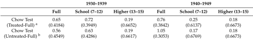
The insignificance and empirical inconsistency of 𝛽 , identified in Figure 3 and Table 1, could also be caused by a negligible share of ‘compliers’ in the full sample; a point made by Oreopoulos (2006) in the context of the CSL effect when using minimum years of schooling indicators, and also mentioned by SY as a possible explanation for their results. We hence investigate whether instrumental validity can be achieved when focusing on a sub-sample with a high complier share. We follow AK’s lead and divide the sample by those obtaining 12 years of schooling (school) and those who obtain more than 12 years of schooling (higher). The former sub-sample has a high share of compliers, while the latter sub-sample comprises mainly always takers. Results are reported and

13 _{CSL indicators based on quarter of birth dummies face similar problems, and Bound and Jaeger (2000) and}

Carneiro and Heckman (2002) show an entanglement of indicators with social status. -0.2 -0.15 -0.1 -0.05 0 0.05 0.1 0.15

IV1 IV2OLS1OLS2 IV1 IV2OLS1OSL2 IV1 IV2OLS1OSL2

610,000 2,166,000 3,680,000

IV1 IV2 OLS1 OLS2

Figure 3.Ordinary least square (OLS) and instrumental variable (IV) estimator consistency. Notes: IV1 and OLS1 are IV and OLS estimates without regional control variables, and IV2 and OLS2 are IV and OLS estimates with regional control variables included. The x-axis provides the sample size and the y-axes coefficient values. The bars indicate the 95% confidence interval. Source: SY, Table1.

Table 1.Sargan and Hausman test for instruments used by SY.

T1A (L_{SY1) T1B (}L_SY2)

White Males Aged 40–49 Aged 25–54 Aged 40–49 Aged 25–54

(1) (2) (3) (4) (1) (2) (3) (4)

β(OLS)a 0.073 ** 0.073 ** 0.063 ** 0.063 ** 0.073 ** 0.073 ** 0.063 ** 0.063 **

βL_(2SLS)a _{0.095 **} −_{0.020 0.097 **} −_{0.014 0.142 ** 0.092 ** 0.140 ** 0.086 **}

Tests: Sarganb

(p-value)

0.99 (0.6088) 4.65 (0.0977) 17.99 (0.0001) 7.51 (0.0234) 0.64 (0.7271) 0.83 (0.6589) 12.75 (0.0017) 17.57 (0.0002) Hausman

(p-value)

3.80 (0.0512) 9.67 (0.0019) 43.24 (0.0000) 36.32 (0.0000) 16.33 (0.0001) 0.53 (0.4671) 150.29 (0.0000) 3.28 (0.0701) Fixed effects:

State of birth Yes Yes Yes Yes Yes Yes Yes Yes

Year of birth Yes Yes Yes Yes Yes Yes Yes Yes

Region x Yob No Yes No Yes No Yes No Yes

Additional

controls: None None

Age quartic, census year Age quartic, census year None None Age quartic, census year Age quartic, census year

Notes: Sargan and Hausman added through replication. Source: SY Tables1andA2.a_{Robust and cluster adjusted}

standard errors are used.b_{Wooldridge’s extension of Sargan’s test of overidentifying restrictions is performed. **}

Significant at the 1% level.

Econometrics2019,7, 36 9 of 20

recession, potentially explaining the low returns to higher education. This effect is concealed in the IV models, given the localness of the CLS instruments.

We now turn to CV to formally compare the two non-nested models (1) versus (3). Figure4shows that the OLS-based models clearly outperform the IV-based models in generalisability, stability, and consistency, even though the CV experiment presented here does not adjust for degrees of freedom.14 Remarkably, results for AK are close to—or even worse than for—SY, despite the finding ofβ≈βL in AK.

Econometrics 2019, 7, x FOR PEER REVIEW 9 of 20

discussed in Appendix A. We do not find stronger evidence for instrument validity but make two interesting observations. Firstly, most IV estimates turn insignificant for the ‘higher’ sub-sample, confirming the high share of always takers. Secondly, OLS estimates reveal shrinking ARTE for those with more years of schooling, especially for the 1940–1949 born cohort. This cohort entered the labour market in the early 1980s in the middle of a recession, potentially explaining the low returns to higher education. This effect is concealed in the IV models, given the localness of the CLS instruments.

We now turn to CV to formally compare the two non-nested models (1) versus (3). Figure 4 shows that the OLS-based models clearly outperform the IV-based models in generalisability, stability, and consistency, even though the CV experiment presented here does not adjust for degrees

of freedom.14 _{Remarkably, results for AK are close to—or even worse than for—SY, despite the}

finding of 𝛽 ≈ 𝛽 in AK.

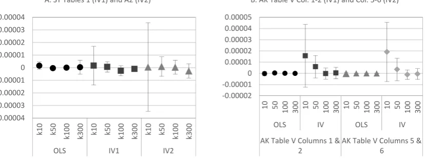
Figure 4. Ratio of average mean square cross validation (CV) error of IV to OLS with Increasing K. Notes: Mean squared error (MSE) is the average of 10 repetitions of the k-fold CV. The curves represent the ratio of the average MSE of the IV model and the OLS counterpart. A value greater than 1 indicates a smaller MSE for OLS than for IV.

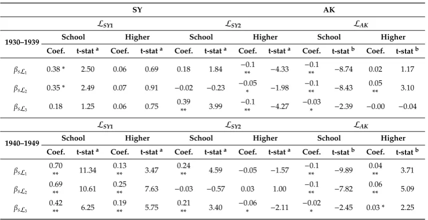
As expected, the MSE decreases as the training sample increases, that is, with increasing k, for both models. However, the IV-based model shows no sign of convergence as training samples grow. When decomposing the MSE into test bias and variance, we find little evidence of asymptotic bias in the OLS estimates; see Figure 5. For the AK case, the IV bias is larger at smaller k and decreases towards no bias at larger k. Given the small bias in general, the large difference in the MSE between the two models clearly stems from a greater variance of the IV model specification, putting the consistency claim of IV into question. While our findings are specific to the CSL case and the chosen instruments, results by Young (2017), who re-evaluates 1359 published IV regressions, suggest that the conclusion drawn from the CV exercise are the norm rather than an exception.

Overall, experimenting with the model design in SY and AK, we find, contrary to what is expected, that the OLS-based model outperforms the IV-based ones in terms of generalisability, stability, and consistency, regardless the choice of CSL indicators.

14 _{The IV approach uses up more degrees of freedom than the OLS counterpart due to the first stage. Therefore,}

the MSE of the IV model specification understates the error when compared to the OLS counterpart.

1.0286 1.02865 1.0287 1.02875 1.0288 1.02885 1.0289 1.02895 1.029 1.0079 1.00795 1.008 1.00805 1.0081 1.00815 1.0082 1.00825

k10 k50 k100 k300

MSE Ratio IV

2

/OLS

MSE Ratio IV

1

/OLS

A. SY Tables 1 (IV1) and A2 (IV2)

IV1 IV2 2.2205 2.221 2.2215 2.222 2.2225 2.223 2.2235 1.0033 1.0034 1.0035 1.0036 1.0037 1.0038 1.0039 1.004 1.0041

k10 k50 k100 k300

MSE Ratio IV

2

/OLS2

MSE Ratio IV

1

/OLS1

B. AK Table V Col. 1-2 (IV1) and Col. 5-6 (IV2)

IV1 IV2

Figure 4. Ratio of average mean square cross validation (CV) error of IV to OLS with Increasing K. Notes: Mean squared error (MSE) is the average of 10 repetitions of the k-fold CV. The curves represent the ratio of the average MSE of the IV model and the OLS counterpart. A value greater than 1 indicates a smaller MSE for OLS than for IV.

Econometrics 2019, 7, x FOR PEER REVIEW 10 of 20

Figure 5. Average CV bias with increasing k. Notes: The CV bias is the average of 10 repetitions of the k-fold CV. Bars on the estimation bias indicate one standard deviation over the 10 repetitions. Numbers of folds shown on the x-axis.

4. Different Income Effects

Section 3 has provided us with no evidence for 𝑠 being in invalid causal variable and we now probe into the causal role of 𝐿. In Section 2, we could distinguish between two income effects: (a) The ARTE effect, 𝛽 . , and (b) the CSL effect or ATE of the CSL via schooling, 𝛽 as specified in (9).

4.1. Estimating ARTE: 𝛽 .

The presentation of varying OLS-based ARTE estimates by AK and SY, despite the use of almost identical samples, indicates problems in the choice of appropriate covariates. Therefore, we proceed with the question of how to specify Z in order to find an empirically adequate specification of (9), which is as parsimonious as possible and can also align the ARTE estimates by AK and SY data, respectively. This is achieved through, firstly, unification of the coding of the education variable and secondly, a parsimonious model specification.

Towards a unification of the education variable, the AK education variable is capped at 17 years to resemble the SY education variable. The unification is found to play a vital role in aligning the ARTE estimates across the two data sets.15 _{We rely on AK’s division between those born in the 1930s}

and 1940s, respectively, using observations from the 1980 census. Towards a more parsimonious model, year of birth dummies included by both AK and SY are replaced with quadratic age (age2).16

Regional dummies for individual states are replaced by a single variable distinguishing between four regions for SY and nine regions for AK data (region). Considering a possible regional effect on school quality, variables capturing school quality (pupilt, term, reltwage) suggested by Card and Krueger (1992a, 1992b) are used by SY and included in our model as well.

Earlier sub-sample experiments, reported in Appendix A, reveal variation in the ARTE estimates with the level of education. The variation reflects ‘sheepskin effects’, which are well documented phenomena in the literature17 _{and clearly discernible in the AK and SY data; see Figure A1 and Table}

15 _{Ideally, we would use uncapped schooling variables, but the transformation in the SY schooling variable is}

irreversible.

16 _{Coefficients on year of birth dummies are found to decline with years, revealing non-linearity. These}

patterns can be almost perfectly replicated with a quadratic age variable. See also Murphy and Welch (1992) for the non-linear relationship between experience and wage earnings.

17 _{See, for instance Angrist (1995); Murphy and Welch (1992); Card (2001); Trostel (2005); and Clark and}

Martorell (2014). This shift in the population education composition also explains the finding by Goldin and Katz (2000). -0.00004 -0.00003 -0.00002 -0.00001 0 0.00001 0.00002 0.00003 0.00004 k1 0 k5 0 k1 00 k3

00 _k10 _k50

k1

00

k3

00 _k10 _k50

k1

00

k3

00

OLS IV1 IV2

A. SY Tables 1 (IV1) and A2 (IV2)

-0.00002 -0.00001 0 0.00001 0.00002 0.00003 0.00004 0.00005

10 50 ₁₀0 ₃₀0 10 50 ₁₀0 ₃₀0 10 50 ₁₀0 ₃₀0 10 50 ₁₀0 ₃₀0

OLS IV OLS IV

AK Table V Columns 1 & 2

AK Table V Columns 5 & 6

B. AK Table V Col. 1-2 (IV1) and Col. 5-6 (IV2)

Figure 5.Average CV bias with increasing k. Notes: The CV bias is the average of 10 repetitions of the k-fold CV. Bars on the estimation bias indicate one standard deviation over the 10 repetitions. Numbers of folds shown on the x-axis.

As expected, the MSE decreases as the training sample increases, that is, with increasing k, for both models. However, the IV-based model shows no sign of convergence as training samples grow. When decomposing the MSE into test bias and variance, we find little evidence of asymptotic bias in the OLS estimates; see Figure5. For the AK case, the IV bias is larger at smaller k and decreases towards no bias at larger k. Given the small bias in general, the large difference in the MSE between the two models clearly stems from a greater variance of the IV model specification, putting the consistency

14 _{The IV approach uses up more degrees of freedom than the OLS counterpart due to the first stage. Therefore, the MSE of the}

Econometrics2019,7, 36 10 of 20

claim of IV into question. While our findings are specific to the CSL case and the chosen instruments, results byYoung(2017), who re-evaluates 1359 published IV regressions, suggest that the conclusion drawn from the CV exercise are the norm rather than an exception.

Overall, experimenting with the model design in SY and AK, we find, contrary to what is expected, that the OLS-based model outperforms the IV-based ones in terms of generalisability, stability, and consistency, regardless the choice of CSL indicators.

4. Different Income Effects

Section3has provided us with no evidence forsbeing in invalid causal variable and we now probe into the causal role ofL. In Section2, we could distinguish between two income effects: (a) The ARTE effect,βys.Z, and (b) the CSL effect or ATE of the CSL via schooling,βyLs as specified in (9).

4.1. Estimating ARTE:βys.Z

The presentation of varying OLS-based ARTE estimates by AK and SY, despite the use of almost identical samples, indicates problems in the choice of appropriate covariates. Therefore, we proceed with the question of how to specifyZin order to find an empirically adequate specification of (9), which is as parsimonious as possible and can also align the ARTE estimates by AK and SY data, respectively. This is achieved through, firstly, unification of the coding of the education variable and secondly, a parsimonious model specification.

Towards a unification of the education variable, the AK education variable is capped at 17 years to resemble the SY education variable. The unification is found to play a vital role in aligning the ARTE estimates across the two data sets.15 We rely on AK’s division between those born in the 1930s and 1940s, respectively, using observations from the 1980 census. Towards a more parsimonious model, year of birth dummies included by both AK and SY are replaced with quadratic age (age2).16 Regional dummies for individual states are replaced by a single variable distinguishing between four regions for SY and nine regions for AK data (region). Considering a possible regional effect on school quality,

variables capturing school quality (pupilt,term,reltwage) suggested byCard and Krueger(1992a,1992b) are used by SY and included in our model as well.

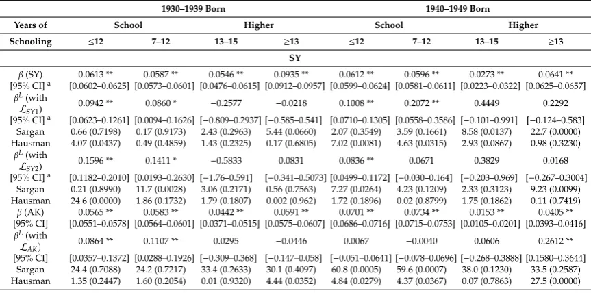
Earlier sub-sample experiments, reported in AppendixA, reveal variation in the ARTE estimates with the level of education. The variation reflects ‘sheepskin effects’, which are well documented phenomena in the literature17and clearly discernible in the AK and SY data; see FigureA1and TableA2, AppendixA. A binary variable (uni) is thus added as a classifier for those who obtained a university degree (15 or more years of schooling).

The key results of this model search are reported in Table2, alongside those from the ‘Original’ models by SY and AK. We refer to our more parsimonious model specifications as ‘Alternative’ in the table. A closer alignment of return to schooling estimates across data sets is achieved with the ‘Alternative’ model specification, which outperforms the ‘Original’ specification in terms of model fit by a margin. OLS estimates point to a relatively constantβys.Zof about 0.06 across data sets and cohorts, and our ARTE estimates are roughly in line with findings byAcemoglu and Angrist(2001), who report estimates of 0.061 and 0.075 respectively.

15 _{Ideally, we would use uncapped schooling variables, but the transformation in the SY schooling variable is irreversible.} 16 _{Coefficients on year of birth dummies are found to decline with years, revealing non-linearity. These patterns can be almost}

perfectly replicated with a quadratic age variable. See alsoMurphy and Welch(1992) for the non-linear relationship between experience and wage earnings.

17 _{See, for instanceAngrist(1995);Murphy and Welch(1992);Card(2001);Trostel(2005); andClark and Martorell(2014). This}

Econometrics2019,7, 36 11 of 20

Table 2.Parsimonious specification of (9).

Original Alternative

SYa _{AK SY}a _AK

1930–1939 1940–1949 1930–1939 1940–1949 1930–1939 1940–1949 1930–1939 1940–1949

βys,Z 0.0751 ** 0.0622 ** 0.0630 ** 0.0519 ** 0.0600 ** 0.0643 ** 0.0576 ** 0.0648 **

[95% CI] [0.074–0.077] [0.061–0.063] [0.062–0.064] [0.051–0.053] [0.058–0.062] [0.063–0.066] [0.057–0.059] [0.064–0.066]

AICb 714,262.9 1,034,376 594,994.7 858,645.2 705,271.2 1,018,112 594,343.4 858,594.8

Adj.-R2 0.0119 −_{0.0232 0.1745 0.1354 0.1217 0.0968 0.1761 0.1355}

Consist.c _{0.0000 0.0000 0.0000 0.0000 0.0000 0.0000 0.0000 0.0000}

Zd _yob31-yob39age2 age3 age4_/yob41-yob49

sob1-sob55

ageq, ageq2, race, married, smsa, neweng midatl, enocent, wnocent, soatl,

esocent, wsocent, mt, year20-year 28

age2, mar, emp, jail, handcap, pupilt, term,

reltwage, uni, region

age2, married, race, smsa, uni, region

Notes: 1980 census, data for SY white male with positive weekly earnings, data for AK male with positive weekly earnings.a_{95% confidence interval based on cluster adjusted standard errors in SY data.}b_{Akaike information}

criteria.c_{Entner et al.(2012) test for consistency. The row reports the correlation coefficient betweenε}

yin (9) and the residuals from the auxiliary regression, with a value close to 0 confirming consistency. Non-Gaussianity of the residuals was tested before and strongly supported by data.d_{See SY and AK for variable names. ** Significant at}

the 1% level.

Following the observations in Table 2, we note that the risk of OVB for βys.Z comes from inadequately specifiedZ. Hence, we evaluate the choice ofZby use of a simple statistical test of consistency developed byEntner et al.(2012). Recalling the DAG in Figure2, we can immediately see that in the presence of OVB, that is, missing covariates inZ, the residualsεyin (9) would be statistically dependent ons.Entner et al.(2012) exploit this insight by means of a simple two-step algorithm to test the consistency ofβys.Zagainst the risk of OVB. In a first step, the key conditional variablesis regressed on the set of covariatesZ.18 If residuals of this auxiliary regression are non-Gaussian—Gaussian residuals are a rarity in large cross-sectional data sets—it is tested for being statistically independent betweenεyfrom (9) and the error term of the auxiliary regression in a second step. If independence is confirmed,βys.Zis consistent with regards to the choice of covariatesZ. The test results are reported in the last row of Table2. In all cases, consistency is strongly supported by the data.

4.2. Estimating the ATE of the CSL via Schooling:βyLs

Given the potential measurement error in CSL indicators identified by SY and briefly discussed in Section3, we follow Section2and conduct two simple experiments to further test the appropriateness of the indicator choice before continuing with the estimation ofβyLs. Since CSL is only binding for school leavers, we would expect the ATE to be insignificant or at least smaller for those with higher education than for those without. Following this reasoning, we estimate the middle equation of (9) using sub-sample groups by educational attainment with the expectation that ˆβsL,0 forSchooland

ˆ

βsL=0 forHigher.

It is shown in Table3that, although ˆβsLtends to be larger for theSchoolsub-sample than for the

Highersub-sample, none of the indicators confirms the hypothesis of ˆβsL=0 forHigher. Noticeably, the size of those ˆβsL,0 in the first cohort has almost doubled that of the second cohort in the case of SY indicators. This shift appears to reflect a general shift towards more years of education. As seen from TableA1(AppendixA), the share of those attaining less or equal the minimum years of schooling is halved in the later cohort.

18 _{The auxiliary regression takes the forms=α}

y+Z

0

βyZ.s+εauxs . Ifεauxs is non-Gaussian, statistical independence between

εaux

Econometrics2019,7, 36 12 of 20

Table 3.βsLin (9) via sub-sampling on educational attainment.

SY AK

L_SY1 L_SY2 L_AK

1930–1939 School Higher School Higher School Higher

Coef. t-stata _{Coef. t-stat}a _{Coef. t-stat}a _{Coef. t-stat}a _{Coef. t-stat}b _{Coef. t-stat}b

βsL

1 0.38 * 2.50 0.06 0.69 0.18 1.84

−_0.1

** −4.33

−_0.1

** −8.74 0.02 1.17

βsL

2 0.35 * 2.49 0.07 0.91 −0.02 −0.23

−_0.05

* −1.98

−_0.1

** −8.43 0.05

** 3.10

βsL

3 0.18 1.25 0.06 0.75 0.39

** 3.99

−_0.1

** −4.27

−_0.03

* −2.39 −0.00 −0.04

L_SY1 L_SY2 L_AK

1940–1949 School Higher School Higher School Higher

Coef. t-stata Coef. t-stata Coef. t-stata Coef. t-stata Coef. t-statb _{Coef. t-stat}b

βsL₁ 0.70

** 11.34 0.13

** 3.47 0.24

** 4.59 −0.05 −1.57

−_0.1

** −9.89 0.04

** 3.71

βsL₂ 0.69

** 10.61 0.25

** 7.63 −0.03 −0.57 0.03 1.00

−_0.1

** −7.82 0.06

** 5.09

βsL₃ 0.42 ** 6.25

0.19 ** 5.75

0.21 ** 3.40

−_0.06

* −2.11

−_0.02

* −2.45 0.03 * 2.25

Notes: 1980 census, data for SY white male with positive weekly earnings, data for AK male with positive weekly earnings. a_{Robust cluster adjusted standard errors.} b_{Robust standard errors. ** Significant at the 1% level.}

* Significant at the 5% level.

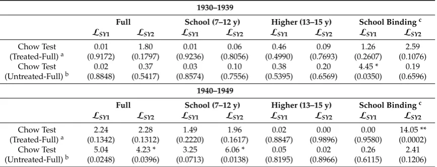
In a second step, we test whether the rule of intervention βyL_.Zs = 0 holds for the different

CSL indicators by estimation of (8) with additional controlsZ. In reference to earlier experiments, we conduct the test for theSchoolsub-sample in addition to the full sample estimation. It is shown in Table4that the conditionβyL_.Zs =0 is validated for SY’sL_SY1indicator across cohorts and also

for AK’sL_{AKindicator for the early born cohort. However, it is violated without exception if using} L_{SY2as CSL indicator. Where conditional independence is rejected in Table4, we have also failed} to confirm ˆβsL=0 for theHighersub-sample in Table3, and rejected instrument validity in Tables1 andA2AppendixA. In cases like this, we should be cautious with the estimate ofβyLs via the chain representation of (10).

Table 4.Test for the rule of interventionβ_yL.Zs=0 using (8) extended byZ.

SYa _AKb

1930–1939 1940–1949 1930–1939 1940–1949

Full School Full School L_AK L_AK

L_SY1 L_SY2 L_SY1 L_SY2 L_SY1 L_SY2 L_SY1 L_SY2 Full School Full School

L₁ −_{0.001 0.041 ** 0.007 0.041 ** 0.014 0.041 ** 0.007 0.046 **} −_{0.007 *} −_{0.008 *} −_{0.01 **} −_0.005

(0.0133) (0.0081) (0.0185) (0.0100) (0.0125) (0.0099) (0.0146) (0.0106) (0.0030) (0.0039) (0.0024) (0.0035) L_{2 0.011 0.028 ** 0.029 0.030 ** 0.016 0.047 ** 0.020 0.052 **} −_0.004 −_{0.009 * 0.012 ** 0.010 **} (0.0139) (0.0062) (0.0189) (0.0078) (0.0126) (0.0081) (0.0142) (0.0085) (0.0030) (0.0039) (0.0024) (0.0035) L_{3 0.021 0.060 ** 0.033 0.063 ** 0.033 ** 0.078 ** 0.031 * 0.082 ** 0.001} −_{0.003 0.012 ** 0.017 **} (0.0144) (0.0103) (0.0196) (0.0113) (0.0122) (0.0122) (0.0140) (0.0124) (0.0030) (0.0038) (0.0023) (0.0034)

Notes: 1980 census, data for SY white male with positive weekly earnings, data for AK male with positive weekly earnings. Zas specified in ‘Alternative’ in Table4. Standard errors reported in parentheses. a_{Robust cluster}

adjusted standard errors.b_{Robust standard errors. ** Significant at the 1% level. * Significant at the 5% level.}

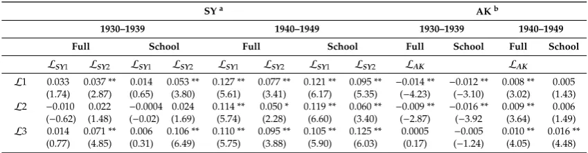
Table5providesβyLs estimated via (10). Where conditional independence is verified, the chain approximation yields significant ATE estimates that confirm our expectation ofβys.Z βyLs. The estimated ATE almost doubles for the later born cohort from 1–3 to 3–5% usingL_{SY1indicators. The} ATE estimates using AK indicators are relatively constant across both sub-samples and cohorts. It should be noted that the negative sign here actually implies a positive ATE, because people born in the first three quartersL1

Econometrics2019,7, 36 13 of 20

to those born in the fourth quarter. The CSL effect is strongest for those born in the first quarter and weakens with the second and third quarter born consecutively.

Table 5.Estimated average treatment effect (ATE) of CSL,β_yLs, using chain models (9) and (10).

SYa _AKb

1930–1939 1940–1949 1930–1939 1940–1949

Full School Full School Full School Full School

L_SY1 L_SY2 L_SY1 L_SY2 L_SY1 L_SY2 L_SY1 L_SY2 L_AK L_AK

L_{1 0.025 ** 0.011 0.022 * 0.011 * 0.054 ** 0.016 * 0.048 ** 0.016 **} −_{0.009 **} −_{0.007 **} −_{0.007 **} −_{0.007 **}

[12.5] [2.56] [6.25] [3.40] [88.4] [6.26] [125] [20.8] [99.2] [75.2] [112] [95.4] L_{2 0.005} −_{0.003 0.021 *} −_{0.001 0.033 **} −_{0.004 0.045 **} −_0.002 −_{0.006 **} −_{0.006 **} −_{0.004 **} −_{0.005 **}

[0.97] [0.12] [6.16] [0.05] [35.4] [0.39] [107] [0.32] [43.4] [70.0] [34.3] [60.4] L_{3 0.004 0.012 0.011 0.023 ** 0.027 ** 0.002 0.028 ** 0.014 **} −_{0.002 *} −_{0.002 *} −_{0.003 **} −_{0.002 **}

[0.44] [3.86] [1.56] [15.9] [20.3] [0.12] [37.8] [11.4] [4.62] [5.68] [15.1] [6.00]

Notes: 1980 census, data for SY white male with positive weekly earnings, data for AK male with positive weekly earnings. See Tables3and4forβys.ZandβsLestimates, respectively. Significance ofβyL_sbased onχ2statistics estimated followingWeesie(1999), reported in brackets. a_{Robust cluster adjusted standard errors.} b_Robust

standard errors. ** Significant at the 1% level. * Significant at the 5% level.

Direct ATE estimatesβyLobtained via (7) exceed estimates obtained via chain approximation for

the later born cohort; see Table6. The effect is indicative of positive indirect CSL effects through control variablesZin later years. Further, chain approximations using SY indicators are much more varied across cohorts than across sub-samples, due to the varying estimates ofβsLin Table3.

Table 6.Estimated ATE of the CSLβ_yLvia (7).

SYa _AKb

1930–1939 1940–1949 1930–1939 1940–1949

Full School Full School Full School Full School

L_SY

1 LSY2 LSY1 LSY2 LSY1 LSY2 LSY1 LSY2 LAK LAK

L_{1 0.033 0.037 ** 0.014 0.053 ** 0.127 ** 0.077 ** 0.121 ** 0.095 **} −_{0.014 **} −_{0.012 ** 0.008 ** 0.005} (1.74) (2.87) (0.65) (3.80) (5.61) (3.41) (6.17) (5.35) (−_{4.23) (}−_{3.10) (3.02) (1.43)} L₂ −_{0.010 0.022} −_{0.0004 0.024 0.114 ** 0.050 * 0.119 ** 0.060 **} −_{0.009 **} −_{0.016 ** 0.009 ** 0.006} (−_{0.62) (1.48) (}−_{0.02) (1.69) (5.74) (2.28) (6.60) (3.40) (}−_{2.87) (}−_{3.92 (3.64) (1.49)} L_{3 0.014 0.071 ** 0.006 0.106 ** 0.110 ** 0.095 ** 0.105 ** 0.125 ** 0.0005} −_{0.005 0.010 ** 0.016 **}

(0.77) (4.85) (0.31) (6.49) (5.75) (3.88) (5.90) (6.03) (0.17) (−_{1.24) (4.05) (4.48)}

Notes: 1980 census, data for SY white male with positive weekly earnings, data for AK male with positive weekly earnings. t-statistics reported in parentheses.aRobust cluster adjusted standard errors.bRobust standard errors. ** Significant at the 1% level. * Significant at the 5% level.

Our finding of a moderate positive ATE of CSL on income (when using labour law indicators) is generally in line with findings reported in the literature; seeAcemoglu and Angrist(2001);Lleras-Muney (2002);Oreopoulos(2006); andGoldin and Katz(2011).

5. What Have We Learnt?

Angrist and Pischke(2015, p. 227) discard theAcemoglu and Angrist(2001) study as ‘a failed research design’ and ascribe the failure to inappropriate CSL indicators, while maintaining the IV approach as appropriate. Conceptualising the IV approach as model choice and experimenting with the data sets used by AK and SY, our analysis exposes nescience about the causal model alternation nature of the IV approach to be the root cause of the failure instead.

Econometrics2019,7, 36 14 of 20

Careful examination of the causal implications of the CSL effects on ARTE by causal chain model representation helps us expose several logical flaws in the conceptualisation of IV-based models. First, it is incorrect to refer toβysLas a consistent estimate of ARTE whensLs. Second, the way in whichsL is generated entangles ARTE with the ATE by CSL in a non-unique manner, reaching deadlock in resolving the ambiguity over the causal interpretation ofβ_ysL. Third, the argument for using IVs to treat measurement errors due to omission of correlated latent variables such as aptitude is unwarranted because ARTE is defined explicitly on education, not aptitude, which entails the specification of ARTA as the parameter of interest.

Experiments with models (9) and (10) show us that relatively robustβys.Zestimates are attainable for ARTE, whereas this is not the case with various ATE estimates. The latter finding tells us that measurement error in CSL indicators is indeed a major concern, a result which confirms the common diagnosis of weak and/or inappropriate IVs in the literature. However, our results warn against the IV route as a dead-end in general when using IV to treat a latent variable problem since, in this case, measurement error in IVs is inevitable and also when prior knowledge suggests the need for explicit multivariate model specification with clear differentiation between moderator and mediator effects; seeArlot and Celisse(2010).

Finally, we find clear guidance and reassurance of our approach from the fundamental concepts and theories in statistical learning. In particular, model bias is identified as the primary source of model-based inferential bias. No theoretically postulated model should be taken as globally correct prior to empirical verification, and structural risk minimisation should be regarded as the key task of empirical studies. Applied research should thus be focused on agnostic probably approximately correct (PAC) learning. Once we fully recognise the untenability of the presumption of theoretically postulated models as globally correct, an implicit presumption underlying the IV-choice over OLS, the methodological defects of this estimator-centred research strategy transpire.

Author Contributions:Conceptualisation, methodology, writing—original draft preparation, writing—review and editing, investigation, resources, formal analysis, software, validation, data curation, visualisation, supervision, project administration, and funding acquisition, D.Q. and S.v.H.

Funding: This research was partly funded by an internal research fund from the Faculty of Law and Social Sciences, SOAS University of London.

Conflicts of Interest:The authors declare no conflicts of interest.

Appendix A

Complier Sub-Sample Experiment

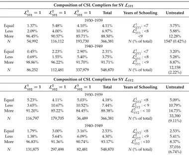
Since most people remain in school beyond the required years, the great majority of the sample belongs to a sub-population for which the ATE of the CSL on schooling is expected to be 0. In other words, the CSL is potentially binding only for school leavers, but by and large not for those who have continued education beyond the compulsory years of schooling. UsingL_{SY2indicators, roughly 4.11%} of the 1930–1939 born cohort complies19 with the law. The share of compliers is even smaller for the later-born cohort with 2.31%. UsingL_{SY2indicators instead, the share of compliers is similarly} small with 4.18 and 2.53% in the 1930s and 1940s birth cohorts, respectively (see TableA1). Our rough estimates of complier shares are slightly lower than inBolzern and Huber(2017), who report a complier share of 6–12% for European countries based on comparison of mean potential outcomes using binary treatment and instrument variables.

19 _{Compliers are overestimated here as the group includes some always takers that would have completed the years of}