Atmos. Meas. Tech., 6, 1673–1683, 2013 www.atmos-meas-tech.net/6/1673/2013/ doi:10.5194/amt-6-1673-2013
© Author(s) 2013. CC Attribution 3.0 License.
EGU Journal Logos (RGB)
Advances in
Geosciences
Open Access
Natural Hazards
and Earth System
Sciences
Open Access
Annales
Geophysicae
Open Access
Nonlinear Processes
in Geophysics
Open Access
Atmospheric
Chemistry
and Physics
Open Access
Atmospheric
Chemistry
and Physics
Open Access
Discussions
Atmospheric
Measurement
Techniques
Open Access
Atmospheric
Measurement
Techniques
Open Access
Discussions
Biogeosciences
Open Access Open Access
Biogeosciences
Discussions
Climate
of the Past
Open Access Open Access
Climate
of the Past
Discussions
Earth System
Dynamics
Open Access Open Access
Earth System
Dynamics
Discussions
Geoscientific
Instrumentation
Methods and
Data Systems
Open Access
Geoscientific
Instrumentation
Methods and
Data Systems
Open Access
Discussions
Geoscientific
Model Development
Open Access Open Access
Geoscientific
Model Development
DiscussionsHydrology and
Earth System
Sciences
Open Access
Hydrology and
Earth System
Sciences
Open Access
Discussions
Ocean Science
Open Access Open Access
Ocean Science
DiscussionsSolid Earth
Open Access Open Access
Solid Earth
Discussions
The Cryosphere
Open Access Open Access
The Cryosphere
DiscussionsNatural Hazards
and Earth System
Sciences
Open Access
Discussions
Retrieving wind statistics from average
spectrum of continuous-wave lidar
E. Branlard1, A. T. Pedersen1, J. Mann1, N. Angelou1, A. Fischer1, T. Mikkelsen1, M. Harris2, C. Slinger2, and
B. F. Montes3
1DTU Wind Energy, Risø Campus, Technical University of Denmark, Roskilde, Denmark 2ZephIR Ltd., The Old Barns, Fairoaks Farm, Hollybush, Ledbury, HR8 1EU, UK 3LM Wind Power, Lunderskov, Denmark
Correspondence to: E. Branlard ([email protected])
Received: 5 November 2012 – Published in Atmos. Meas. Tech. Discuss.: 19 February 2013 Revised: 17 May 2013 – Accepted: 6 June 2013 – Published: 15 July 2013
Abstract. The aim of this study is to experimentally
demonstrate that the time-average Doppler spectrum of a continuous-wave (cw) lidar is proportional to the probability density function of the line-of-sight velocities. This would open the possibility of using cw lidars for the determina-tion of the second-order atmospheric turbulence statistics. An atmospheric field campaign and a wind tunnel exper-iment are carried out to show that the use of an average Doppler spectrum instead of a time series of velocities de-termined from individual Doppler spectra significantly re-duces the differences with the standard deviation measured using ordinary anemometers, such as ultra-sonic anemome-ters or hotwires. The proposed method essentially removes the spatial averaging effect intrinsic to the cw lidar systems.
1 Introduction
Doppler lidars cannot precisely estimate the wind veloc-ity fluctuation statistics in comparison to ordinary sonic anemometers because of the relatively large averaging vol-ume. Many engineering applications such as the load estima-tion on buildings, and in particular loads on wind turbines, use point-wise measurements to characterise the turbulence at the site of the structure. To be consistent with the building and the wind turbine codes, it is desirable to have the lidars compensate for the averaging effect.
Many authors devise methods to measure turbulence statistics such as spectra, variances or the energy dissipation. The methods for estimating the energy dissipation (Frehlich
above investigations, the Doppler velocity is derived from the Doppler spectrum and then a statistical analysis of these Doppler velocities is carried out. In the present contribution, we average the Doppler spectra directly without calculating the Doppler velocities first. Following this approach, Mann et al. (2010) devised a method to circumvent the averaging effect completely for the vertical flux of the horizontal mo-mentum for a conically scanning cw lidar. The method was based on the assumption that the Doppler spectrum averag-ing over an extended time period is equal to the probability density function (pdf) of the weighted LOS velocities in the measurement volume. The velocities are adjusted with a cer-tain weighting, which for an untruncated, focused Gaussian beam is well approximated by a Lorentzian function (Son-nenschein and Horrigan, 1971).
The purpose of the present study is to experimentally ver-ify the assumption that the average Doppler spectrum of a cw lidar is proportional to the pdf of the LOS velocities in order to promote the possibility of using lidars for precisely esti-mating the second-order turbulence statistics.
A field measurement campaign was carried out at Risø where a ZephIR prototype (Smith et al., 2006) was mounted on a parked Vestas V27 turbine nacelle staring horizon-tally upwind towards a mast-mounted sonic anemometer (Angelou et al., 2012b).
A wind tunnel experiment was performed in order to in-vestigate what other effects other than turbulence might con-tribute to the width of the mean Doppler spectrum. Further, in the wind tunnel, by adding a grid, we generated turbu-lence with a small length scale of the order of a few centime-tres. Under these conditions the averaging effect of the lidar was considerably larger than in the field experiment and the advantage of deriving turbulence statistics from the average Doppler spectrum was more evident.
Following the work of Mann et al. (2010) the method and assumptions used for determining the wind statistics from the Doppler spectra are presented in Sect. 2 along with consid-erations about possible additional spectral broadening. Some practical aspects of the manipulation of raw Doppler spectra are discussed in Sect. 3. In Sects. 4 and 5, the field and wind tunnel experiments are described, followed by a presentation of the different results and discussions.
2 Lidar Doppler spectra for wind analysis
Commercial Doppler lidars are commonly used as anemome-ters in which the velocity is directly calculated by the internal software provided by the lidar’s manufacturer. This velocity is obtained from the Doppler spectrum by various estima-tion techniques. The use of Doppler spectra for accessing the statistics of the LOS velocity at the focus point of the lidar will be discussed. Under some assumptions, it will be seen that the spatial averaging of the lidar can be circumvented.
2.1 Lidar Doppler spectra
The LOS is oriented by a unit vector nin the direction of emission. The beam waist or focus point is located at a posi-tionxin space corresponding to a radial positions=0 along the LOS. The radial velocity (or LOS velocity) measured by the lidar is assumed to be a weighted average of all the ve-locities along the LOS; therefore,
vr(x)=
∞ Z
−∞
ϕ(s)n·u(sn+x)ds, (1)
whereϕ is the lidar weighting function anduis the three-dimensional velocity field. For the ZephiR lidar, and for any well constructed cw lidar, this function is well approx-imated by a Lorentzian (Smith et al., 2006; Angelou et al., 2012b). The lower limit of the integration should rigorously correspond to the position of the lidar. It is taken here as
−∞for simplicity. This choice is also convenient since the Lorentzian function does not have a compact support. Nev-ertheless, this limit could be replaced by the position of the lidar if it is ensured that the weighting function is normalised to unity on the integration domain. This is the property of the weighting function used in Sect. 2.2.
In practice, the lidar measures the frequency difference 1f between the emitted beam and the back-scattered radi-ation from atmospheric aerosols. To assess this frequency difference, the beat signal between the local oscillator and the backscattered radiation is Fourier transformed and abso-lute squared in order to obtain a spectrum denoted asS(f ). The determination of the centre frequency is not completely straightforward as discussed in Sect. 3.1. The frequency shift assessed into the spectral domain is converted to the wind radial velocityvr(x)using
1f f =2
vr
c ⇒vr= 1
2λ1f, (2)
withf,λandcbeing the lidar frequency, lidar wavelength, and speed of light, respectively. Using Eq. (2), we can ex-press the Doppler spectrum in terms of velocity:S(vr).
2.2 Average lidar Doppler spectra
In this section, the mathematical formalism related to the time averaging of the Doppler spectra is introduced.
Mann et al. (2010) made a simple assumption about the connection between spectrum and velocity distribution: the Doppler power spectral density corresponding to a given ve-locityv˜r is taken as the sum of the contributions of all the radial velocities equal tov˜ralong the beam weighted by the spatial averaging functionϕ:
S(v˜r)=
∞ Z
−∞
The tilde notation will be further dropped for simplicity. It should be noted that in the above equation, the spectrum is assumed to be normalised to unity for the sake of simplicity. The Doppler spectra are averaged for a given period, and this time averaging is denoted byh. . .i. The average spectrum is as follows:
hS(vr)i =
∞ Z
−∞
ϕ(s)p(vr|s)ds, (4)
wherep(vr|s)is the probability density function (pdf) of the radial velocities at a radial positionson the beam during the time period investigated.
Mann et al. (2010) pointed out that if the pdf of the veloc-ities does not depend on the positions, thenp(vr|s)=p(vr) and Eq. (4) becomes:
hS(vr)i =p(vr) . (5) In the two experiments considered in this paper, the beam direction is in a homogeneous direction, meaning that the statistics of the velocity does not change along the beam, and Eq. (5) is valid. In Mann et al. (2010), the mean wind speed changes along the beam; hence, ifp(vr|s)depends on s, Eq. (4) must be used instead of Eq. (5).
2.3 Other sources of spectral broadening
Scanning the lidar beam through the atmosphere or staring at an angle as compared to the direction of the wind flow will lead to spectral broadening of the signal even if the flow itself is perfectly homogeneous. This is essentially because the time a scattering particle (or aerosol) is illuminated by the lidar beam is limited. The bandwidth of the signal is inversely proportional to the time that an aerosol takes to move through the beam diameter. We perform a simplified analysis of how this affects the spectrum by assuming that the aerosol passes the beam close to the focus. We ignore the Doppler shift itself and focus on the width of the Doppler spectrum.
The cross section of the electric field in the focus point of the beam can be described by a centred Gaussian
E(x)∝exp
" −
x
w0
2#
, (6)
wherew0is the beam waist radius (1/e2 half-width) of the optical power, which is the square of the electrical field, and x is the position perpendicular to the beam. The time scale for a scatterer moving perpendicular through the beam waist is
τ= w0
vpart
, (7)
wherevpart is the relative velocity between the focus point and the particle. The voltage, generated by the detector, will
also be a Gaussian as a function of time
V (t )∝exp
" −
t−t
0 τ
2#
, (8)
wheret0is the random timing of the aerosol transit. In the frequency domain, the detector output becomes
V (f )∝exph−(π τf )2iexp [2πif t0], (9) and hence, the power spectrum S(f ), which is the mean absolute square of the above, becomes proportional to exp
−2(π τf )2. Therefore, the 1/e2 full-width, or the so-called spectral bandwidth, is
fBW= 2 π τ =
2vpart π w0
. (10)
An additional effect that widens the Doppler spectrum is the finite timeT used as a window in the Fourier analysis of the detector signal. Now, the detector signal becomes
V (t )∝exp
" −
t−t
0 τ
2#
5(t /T ), (11)
where 5(t /T ) is the rectangle function, i.e. 1/T for t∈
[−T /2, T /2] and zero otherwise. The Fourier transform of Eq. (11) is
V (f )∝
T /2
Z
−T /2 exp
" −
t−t
0
τ
2#
exp [−2π i f t] dt
∝ exp [2πif t0] exp
h
−(πf τ )2i (12)
×
erf
1
2 T τ −
t0 τ −iπf τ
−erf
1
2 T τ +
t0 τ +iπf τ
,
where erf is the error function of a complex argument. Taking the mean square of this equation implies averaging over the random timet0, so
S(f )∝exph−2(πf τ )2i× ∞ Z
−∞
erf
1
2 T τ −
t0 τ −iπf τ
+erf
1
2 T τ +
t0 τ +iπf τ
2
dt0, (13)
The derivation presented here is only approximate. The purpose of the derivation is to show the proportionality under non-turbulent flow conditions of the Doppler spectral width with the wind speed as expressed in Eq. (10), and the small additional offset due to the Fourier analysis timeT.
3 Problems raised by the manipulation of raw spectra
3.1 Determination of the frequency
Determining the radial velocity vr from the lidar Doppler spectrum is in reality more complex than stated in Eq. (2). The averaging of the Doppler spectra allows a better signal-to-noise ratio, and this first averaging step is carried out inter-nally by the lidar. Once the signal is sufficiently significant, the challenge lies in the determination of the main frequency of the spectrum. The different techniques employed by the manufacturers are beyond the scope of this paper. Neverthe-less, a method to determine the main frequency of the spec-trum had to be used for this study and a choice had to be made between three different methods. First, the frequency can be considered to correspond to the maximum power spec-tral density. Secondly, the frequency can be considered the barycenter of the power density. Finally, the frequency can be determined as the median of the spectrum. This last method has been used in the analysis of the lidar spectra presented here to determine the lidar wind speed time series (also see Angelou et al., 2012a). It should be noted that the analyti-cal development of Sect. 2.1 and Eq. (1) use the barycenter definition. The barycenter definition is easier to handle ana-lytically, but the median method is seen to be less noisy in practice (Angelou et al., 2012a).
3.2 Different scaling for the lidar spectra
Post processing of the raw ZephIR lidar spectra is required prior to the application of the frequency estimator method used to derive the Doppler shift. The first step is to divide the spectrum with the background noise spectrum in order to obtain a flat background. Then, the background noise of the spectrum is removed, and for convenient storage, the signals are scaled so that they take values in the same range. These two steps are performed as follows:
Each frequency spectrumS(f )output by the lidar is scaled and stored in a database according to
SDB(f )=255×
S(f )−Snoise Smax−Snoise
=αS(f )+β. (14)
The noise threshold levelSnoiseis determined by an interval away from the frequency corresponding to the maximum of the spectrum Smax. The Doppler shift signal is indeed ex-pected to be where the spectrum is maximum so that far from this maximum, the spectrum consists of the flat back-ground noise. The noise threshold is given by the mean plus, somewhat arbitrary, three times the standard deviation of the
spectrum on this interval (Angelou et al., 2012a). The spectra stored in the databaseSDBtake values between 0 and 255.
At this stage, all database spectra have the same amplitude for a convenient storage, but prior to averaging them over ten or thirty minutes, the spectra are scaled a second time by di-vision with another scaling factorα∗. For this second stage three different scaling methods are considered. The first pos-sibility is to keep the database spectra as they are (α∗=1) implying the same contribution to the average spectrum from signals with low backscatter and signals with high backscat-ter. Another possibility is to scale back the database spectra to get to the original lidar spectra without noise (α∗=α). Finally, the third option involves normalising each spectrum by its area (α∗=RSDB(f )df) assuming a constant energy content for all the spectra. After scaling, the frequency spec-tra are converted to velocity specspec-tra according to Eq. (2), then averaged over a given period, typically 30 min, and nor-malised to have unit area. All methods were tested on the field experiment described in Sect. 4, and as later described the last method was slightly superior, and was applied for the wind tunnel experiment in Sect. 5.
4 Field experiment
The field experiment used to validate Eq. (5) and show the benefit of analysing average Doppler spectra for turbulence statistics will be described in this section.
From April 2009 to December 2009 a measurement cam-paign was carried out at the DTU Risø campus test site where a ZephIR prototype lidar was mounted on the na-celle of a Vestas V27 wind turbine staring horizontally. Dur-ing one day, the turbine was stopped and its yaw locked so that the laser beam focused 1 m above a Metek USA sonic anemometer measuring at 32 Hz and located on a meteo-rological mast 67.5 m from the lidar. The two instruments were covering exactly the same time interval and the mea-surement volumes were almost co-located which facilitates the comparison of turbulence statistics between the instru-ments. The Metek sonic was corrected offline according to the wind-tunnel-based calibration provided by the manufac-turer (Berg et al., 2011). The sampling rate of the lidar is 100 MHz which leads to a velocity resolution of roughly 0.15 m s−1using 512 pt FFT. Refer to Angelou et al. (2012b) for further details.
from the fibre laser and centred at around 1 MHz dominates the lidar spectrum at low frequencies (Cariou et al., 2006). This leads to a decrease in signal-to-noise ratio and makes it more difficult to assess the Doppler shift. The effect of RIN can be cancelled by using balanced photo detectors in the li-dar, or possibly a laser with active RIN suppression (Spiegel-berg et al., 2004). Excess RIN has been eliminated from the current generation of ZephIR lidars, which operate close to the shot noise limit across the full speed range. The thresh-old of 4 m s−1was chosen to match the usual value of wind turbines cut-in wind speed.
In this experiment, the lidar stared horizontally over a ter-rain that had a slight slope of the order of 2 %. As the first ap-proximation it was assumed that the flow was homogeneous along the LOS. The relationp(vr|s)=p(vr)was hence as-sumed, and data from this experiment were used for validat-ing Eq. (5).
5 Wind tunnel experiments
Two experiments, one with and the other without turbulence, were carried out in a wind tunnel.
5.1 Turbulence
To verify the expression given in Eq. (5), a comparison study between a hotwire anemometer (HW) and a short-range cw lidar was performed in an aerodynamic wind tun-nel. The wind tunnel had a test section with the dimensions of 7×2.7×1.35 m3and was capable of delivering wind speeds up to 100 m s−1 (Fischer, 2012). To create a turbulent air-flow, a metal grid was placed in the inlet of the test section. The HW was a 2-D X-wire probe (Dantec 55P61), and it was placed in the middle of the wind tunnel test section measur-ing two perpendicular components of the wind velocity, one along the wind and the other in the transverse direction, at a rate of 25 kHz (Fischer, 2012). The lidar was a ZephIR 300 cw lidar modified to measure high wind speeds of up to 80 m s−1. The sampling frequency and velocity resolution of the lidars used for the field and wind tunnel experiment are identical. However, the most important modification was the replacement of the standard telescope unit with a smaller and externally connected telescope. This telescope had a 1-inch(2.54 cm) lens that gave the lidar a measurement range of approximately 1–10 m and was connected to the laser and signal processing unit through a 35 m optical fibre duplex ca-ble such that it could be mounted inside the wind tunnel with a bulky base unit placed outside (Pedersen et al., 2012). The lidar stared horizontally into the wind with the waist of the laser beam placed approximately 2 cm above the HW.
Two series of tests were conducted in which the tunnel was set to deliver a mean wind speed of 45 and 55 m s−1, re-spectively. The hotwire recorded data for 83.9 s at a rate of 25 kHz while the lidar sampled for 60 s at 50 Hz. From the
HW data, the velocity component in the staring direction of the lidar was calculated, and from this, the pdf was subse-quently calculated by dividing the range from 41–47 m s−1 (or 51–57 m s−1) into 100 bins and counting the occurrences. For the lidar, two different approaches were used. In the first approach, the ensemble averaged mean spectrum was calcu-lated as described in Sect. 2.2. In the second approach, one wind speed is calculated from each 50 Hz Doppler spectrum using the median method, and then, the pdf was found as for the HW. It should be pointed out that the determination of the median was not restricted to bin values, intermediate values using linear interpolation were allowed.
5.2 Doppler spectral width in laminar flow
To experimentally examine the spectral broadening due to reduced dwell time, the lidar was placed in the wind tunnel without the grid such that a laminar flow was achieved. This time a telescope with a 2-inch (5.08 cm) lens was used, and the lidar beam was focused at a distance of 1.05 m, well in-side the boundaries of the test section, and pointed down-wards at an angle of 66.5◦ as compared to the horizontal wind flow. The short focus range resulted in a tight focus with a waist radius of 52 µm, but because of the angle be-tween the direction of the beam and the flow, the effective waist radius was 57 µm. Using this value for the waist radius, we could rewrite Eq. (10) as
fBW=11163 m−1·vpart. (15)
The wind speed was ramped up from 10 to 70 m s−1in steps of 10 m s−1, and the data were collected for two minutes in each step. The lidar sampled 50 spectra per second, and af-ter spectra not containing a wind signal were discarded, ap-proximately 5820 usable spectra were obtained for each step. The spectra were then ensemble averaged as described in Sect. 3.2 and subsequently a Gaussian distribution was fit-ted by a least-squares technique to obtain the width.
6 Results
8 10 12 14 0.00
0.05 0.10 0.15 0.20 0.25 0.30 0.35
Wind speed@msD
@
s
m
D
Sonic PDF Lidar Avg. Spectrum
Fig. 1. Comparison of sonic pdf with the corresponding lidar aver-age spectrum for a period of 30 min.
An example of the comparison between the sonic pdf for a given period and the corresponding lidar spectrum is shown in Fig. 1. As can be seen, the curves correlate to a high degree but a small shift is observed. This shift is found from the small difference in the mean wind speed measured by the two instruments. This will be further investigated in the following paragraphs.
6.1 Comparisons of statistical moments
The mean is derived from the pdf as
µvr=
∞ Z
−∞
vrp(vr)dvr, (16)
and the standard deviation as
σv2 r=
∞ Z
−∞
vr−µvr
2
p(vr)dvr. (17)
Using the wind speed time series from the lidar and the sonic anemometer, we find that these moments correspond exactly to the moment obtained by using ensemble averaging over the studied period, which isµvr= hvriandσ
2
vr= hv
2
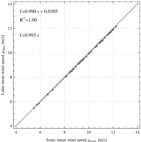
ri−hvri2. The comparison of the mean radial velocity from the lidar and the sonic shows a really high correlation with a slope of 0.993 as shown on Fig. 2. A slightly inferior slope of 0.992 is found by comparing the mean from the average spectrum calculated with Eq. (16) and the time series of the sonic anemometer. As seen in Fig. 1, this small shift in the mean wind speed is visible when comparing the two pdfs. As a result, the small difference in mean is corrected for further comparisons of the pdfs. The difference in mean is discussed in Sect. 7. The results for the field experiment concerning the standard deviation will be presented in Sect. 6.3.
æ æ
æ ææ
æ
ææææ æ æ
æ æ
æ æ
æ
æ æ æ æ æ æ
æ æ
ææ æ æææ
æ
æ
æ æ
æ æ
æææ æ
æ æ
æ æ
æ
f=0.990 x+0.0305
R2=1.00
f=0.993 x
4 6 8 10 12 14
4 6 8 10 12 14
Sonic mean wind speedΜsonic@msD
Lidar
mean
wind
speed
Μlidar
@
m
s
D
Fig. 2. Comparison of half-hour averages of the LOS velocity from the lidar and the corresponding velocity component of the sonic. Expressions for a linear fit with and without an offset are shown. Data are obtained during the day of 5 May 2009.
6.2 Comparison of sonic pdf with average lidar spectra
Averaging periods from 30 s to 30 min have been investigated for comparisons with the sonic pdf. Results for 10 min or 30 min periods are presented in the following paragraphs as they are reasonable periods for evaluating turbulence statis-tics and their resulting pdf is relatively smooth. A correla-tion method is presented to quantify the similarity between the sonic pdf and the average Doppler spectrum. As the first means of comparison, the sonic pdf and the average spectrum are plotted above each other as shown in Fig. 3. This insta-tionary case corresponds to a 30 min period where the ra-dial velocity decreased significantly, thus explaining the ob-served double spikes. The correction for the small difference in mean is taken into account for these plots and it can be seen that the curves agreement is remarkable. Such graphical comparisons were performed for 13 30 min periods and 46 10 min periods, showing similar results.
8 9 10 11 12 13 14 15 0.0 0.1 0.2 0.3 0.4 0.5 0.6
Wind speed@msD
PDF @ s m D Sonic PDF Lidar Avg. Spectrum Lidar PDF
Fig. 3. Similar to Fig. 1, but for another 30 min period. Sonic
veloc-ities have been multiplied with 0.993 in order to compensate for the
imperfect calibration shown in Fig. 2. The pdf from the lidar time series (Lidar PDF) has been added to the figure.
æ æ æ æ æ æ ææææ æ æ æ æ æ æ æ æ æ æ æ æ æ æ ææææææææ æ ææææææ ææ æ æ æ æ æ à à à à à à à à àà à à à à à à à à à à à à à à à à à à à à à à à à à à à à à à à à à à à à
4 6 8 10 12 14
0.96 0.97 0.98 0.99 1.00
Radial Velocity@msD
Correlation
coefficient
@
.
D
Lidar Avg. Spectrum Lidar PDF-Mean:
æ à
Mean value: 0.995 Mean value: 0.984
Fig. 4. Comparison of the lidar pdf and the lidar average spectrum with the sonic pdf by a correlation analysis. The radial velocity is the LOS velocity averaged over 10 min.
the results for the method of scaling per area are shown. The correlation from the lidar wind speed time series pdf showed the lowest correlation with an average coefficient of 98.4 %, whereas the average spectra showed an average of 99.5 %. Among the different scaling methods, the method of scaling by area exhibited the best correlation results with a correla-tion coefficient 0.1 % higher than the next best method.
A common method used for comparison of probability distributions is the Kolgomorov-Smirnov(KS) test which is based on the maximum distance between two cumulative dis-tribution functions(cdf). The correction on the mean is ap-plied since it is not an inherent feature of the pdf but consid-ered as a measurement error. Results are shown in Fig. 5 us-ing averagus-ing periods of 30 min. Consistent with the correla-tion analysis, the KS test reveals that the distance between the sonic cdf and the average spectrum cdf is in average smaller than the distance between the sonic cdf and the lidar time series cdf. æ æ æ æ æ æ æ æ æ æ æ æ æ à à à à à à à à à à à à à
0 2 4 6 8 10 12
0.00 0.01 0.02 0.03 0.04 0.05
Time period index
KS test @ s m D
Lidar Avg. Spectrum Lidar PDF
æ à Mean value: 0.022
Mean value: 0.012
Fig. 5. Kolgomorov–Smirmov test for the two lidar statistical dis-tributions with respect to the sonic cdf using 14 30 min periods.
These results confirm what was seen graphically, i.e. the average Doppler spectrum and the sonic pdf correlates to a high degree, which in turn confirms that the assumption of a constant probability density function along the horizontal LOS is fair. Further, this comparison showed that the aver-age Doppler spectra showed closer resemblance to the sonic pdfs than the lidar pdfs did. The potential of the method in circumventing the effect of the spatial averaging will be fur-ther emphasised by the results of the wind tunnel experiment.
6.3 Standard deviation
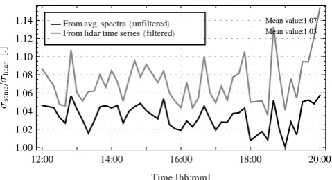
The interesting aspect of the analysis of the Doppler spectra under the assumption of a constant probability density func-tion of the radial velocities along the LOS lies in the fact that the spatial averaging is removed. In this case, the spatial av-eraging inherent to the physics of the lidar disappears when the lidar spectra are averaged, whereas it is present when the lidar wind speed time series is used. This issue is critical for the determination of turbulence statistics. It has been ob-served and derived that the standard deviation measured by the lidar has an inherent systematic error due to this spatial averaging (Mann et al., 2009; Sj¨oholm et al., 2009; Angelou et al., 2012b). To illustrate the benefit of the present method, the wind speed standard deviation obtained from the lidar time series is compared to the standard deviation calculated using Eq. (17) on the average Doppler spectra. The standard deviations obtained are expressed with respect to the stan-dard deviation measured by the sonic anemometer as shown in Fig. 6.
12:00 14:00 16:00 18:00 20:00 1.00
1.02 1.04 1.06 1.08 1.10 1.12 1.14
Time@hh:mmD
Σsonic
Σlidar
@
.
D
From avg. spectraHunfilteredL From lidar time seriesHfilteredL
Mean value:1.07 Mean value:1.03
Fig. 6. Comparison of standard deviations obtained from the lidar time series (gray) and from the average Doppler spectrum (black) with respect to the sonic standard deviation.
6.4 Wind tunnel turbulence
We now present the results from a similar comparison in the wind tunnel.
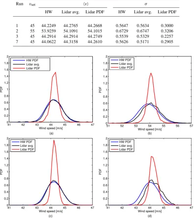
Figure 7a shows the resulting pdfs based on the HW (blue) and lidar (green and red) measurements as described above. All three measurements find essentially the same mean wind speed of approximately 44.3 m s−1(see Table 1), but clearly the width of the pdf based on wind speeds from velocity determination from individual Doppler spectra (red) stands out from the other two. This pdf is considerably narrower than the other two with a standard deviation of 0.30 m s−1 as compared to 0.56 m s−1. This is due to the spatial averag-ing inherent to the lidar as described above. The agreement between the HW pdf and the lidar mean spectrum is remark-able. This can be quantified for instance by analysis of their widths which are 0.5647 and 0.5634 m s−1, respectively.
The same tendency is clearly seen in Fig. 7b showing the results of the second test series where the tunnel was set to deliver a mean speed of 55 m s−1. Again, the widths of the HW pdf and the lidar average spectrum are found to be in high correlation with standard deviations of 0.6729 and 0.6747 m s−1, respectively, while the lidar pdf is consider-ably narrower with a width of 0.3206 m s−1. However, it is also seen that the mean wind speeds estimated by the HW and the lidar deviate by approximately 0.18 m s−1from each other or by approximately 0.3 %.
Table 1 summarises the results for all turbulence runs in the wind tunnel. The wind tunnel is equipped with a heat exchanger, which, as a side effect, removes aerosols. There-fore, a tiny quantity of smoke was introduced into the tunnel flow prior to the experimental runs. The sequence of runs in Table 1 thus corresponds to smaller and smaller aerosol load-ing. The average wind speeds derived from the lidar average Doppler spectrum and the histogram of lidar velocities are, as expected, virtually identical. The difference from the mean from the hotwire varies from 0 to 0.6 %. The standard devi-ations from the average Doppler spectra are vastly superior
to the ones obtained from the time series of lidar velocities. The performance of the lidar deteriorates from run 1 to run 7 most probably because the particle concentration in the wind tunnel decreases as a function of time. This progression can also be seen on the pdfs shown in Fig. 7a–d.
6.5 Laminar wind tunnel flow
We now discuss the very narrow Doppler spectra obtained in the non-turbulent experiments in the wind tunnel. Fig-ure 8 shows the ensemble mean of the 5824 valid spectra recorded at the pre-set speed wind speed of 50 m s−1, which is the equivalent to 45.3 m s−1 perpendicular to the beam. The Gaussian fit used for deriving the width of the average Doppler spectrum is also shown.
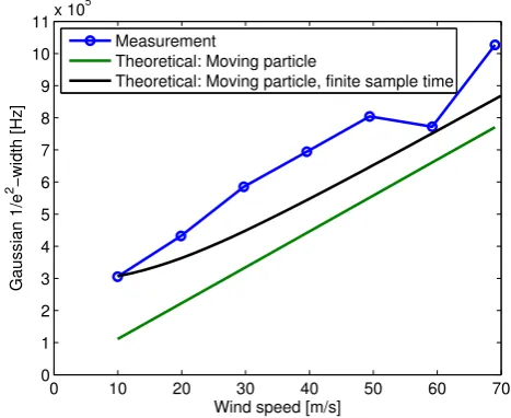
The procedure for obtaining the width is now repeated for every wind speed. Fig. 9 shows the 1/e2width of the fitted Gaussian as a function of wind speed perpendicular to the beam together with the simple theoretical prediction given in Eq. (15) and the prediction based on Eq. (13). The distribu-tions are seen to be slightly wider than those predicted by Eq. (13). A possible explanation for this is that the flow in the wind tunnel may not be completely laminar, which could add to the width. According to Fischer (2012), the turbulence level in the “laminar” wind tunnel is very difficult to mea-sure, but it seems that it is less than 0.2 %. For a mean wind speed of 50 m s−1, it would correspond to a maximum stan-dard deviation of 0.1 m s−1. This corresponds to a frequency shift of 132 kHz, which is of the same order as the difference between the theoretical and the measured values. Therefore, by comparing the measurements and the theoretical curve of Fig. 9, we cannot rule out the possibility that weak veloc-ity fluctuations in the wind tunnel account for the additional spectral width.
7 Discussion
The cw lidars used in these investigations performed at least as well as other similar investigations with respect to the mean wind speed (Wagner et al., 2011; Gottschall et al., 2012). The differences in the mean measured by the sonic are generally less than 1 %, and around 0.1 % for the hot-wire in the wind tunnel. These small differences are of no concern here. It is the ability of the cw lidar to measure wind fluctu-ations by the use of the average Doppler spectrum, which is the central issue of this paper.
Table 1. Mean wind speeds and widths for the different instruments and analysis methods. Dimensional variables are in metres per second.
Run vset hvi σ
HW Lidar avg. Lidar PDF HW Lidar avg. Lidar PDF
1 45 44.2249 44.2765 44.2668 0.5647 0.5634 0.3000
2 55 53.9259 54.1091 54.1015 0.6729 0.6747 0.3206
3 45 44.2914 44.2914 44.2749 0.5539 0.5329 0.2257
7 45 44.0622 44.3158 44.2610 0.5626 0.5171 0.2905
41 42 43 44 45 46 47
0 0.2 0.4 0.6 0.8 1 1.2 1.4 1.6 1.8 2
Wind speed [m/s]
HW PDF Lidar avg. Lidar PDF
51 52 53 54 55 56 57
0 0.2 0.4 0.6 0.8 1 1.2 1.4 1.6 1.8 2
Wind speed [m/s]
HW PDF Lidar avg. Lidar PDF
41 42 43 44 45 46 47
0 0.2 0.4 0.6 0.8 1 1.2 1.4 1.6 1.8 2
Wind speed [m/s]
HW PDF Lidar avg. Lidar PDF
41 42 43 44 45 46 47
0 0.2 0.4 0.6 0.8 1 1.2 1.4 1.6 1.8 2
Wind speed [m/s]
HW PDF Lidar avg. Lidar PDF (a)
(c)
(b)
(d)
Fig. 7. The pdfs based on the HW and lidar measurements together with the ensemble averaged lidar spectrum and the pdf obtained from the lidar wind speed time series. The four figures (a-d) correspond respectively to run 1, 2, 3 and 7. See Table 1.
derived velocities, see for example Fig. 7a, implying that the spatial averaging could be circumvented. Yet differences in standard deviations of the order of 3 % are found between re-sults from the averaging spectra method and the sonic mea-surements. Several factors could influence the method and explain these differences, mainly: the assumptions leading to Eq. (3), the noise suppression method and the scaling method of the spectra. In the wind tunnel experiment, the difference between the methods of obtaining turbulence statistics from the lidar is very pronounced because in this case, the scale of the turbulence is of the order of the full-width half-maximum
2.45 2.5 2.55 2.6 x 10⁷ 0
0.2 0.4 0.6 0.8 1
Frequency [Hz]
PSD
Measurement Gaussian fit
Fig. 8. Example of ensemble averaged Doppler spectrum together
with a Gaussian fit obtained at a nominal wind speed of 50 m s−1.
We have also shown that neither the transit time nor the finite time period of the Fourier analysis significantly widens the average Doppler spectrum. For wind speeds perpendic-ular to the laser beams of 70 m s−1, spectral widths of up to 1 MHz were observed, but that relatively large width was obtained for an extremely small beam radius and in a very homogeneous flow. For very low wind speeds, the spectral width is dominated by the rectangular window function im-posed by the sampling of the signal. This width is less than two frequency bins in the digitised spectrum and is thus con-siderably smaller than what is usually seen in the measure-ments of atmospheric wind speeds. Though present for the laminar case of the wind tunnel experiment, the effect of FFT-windowing is not significant for the general case of tur-bulence in the atmosphere. For a conically scanning cw lidar, wind speeds perpendicular to the beam can easily exceed the maximum speed tested here because of the normally long fo-cus ranges and resulting circumference of the scanned disc. However, a relatively long focus range will also lead to a rel-atively large beam waist radius. For example, for a ZephIR lidar focused at 100 m and with a scan rate of 1 s, the tan-gential scan speed will be approximately 160 m s−1, but the waist radius of approximately 2 mm and the spectral band-width will be dominated by the window function. Notice also that because the tangential speed and the waist radius both increase linearly with focus distance, this is true for all ranges. Therefore, for spectral broadening to severely af-fect the recorded Doppler spectrum substantially higher scan rates are required.
For the method of average Doppler spectrum to be rel-evant, it must be applicable in situations where the flow changes statistically along the laser beam. This was shown in Mann et al. (2010) for some statistics including the co-variance between the horizontal and vertical velocity
com-0 10 20 30 40 50 60 70
0 1 2 3 4 5 6 7 8 9 10 11x 10
5
Wind speed [m/s]
Gaussian 1/e
2 −width [Hz]
Measurement
Theoretical: Moving particle
Theoretical: Moving particle, finite sample time
Fig. 9. Spectral bandwidth as function of wind speed. The measured values are represented by the dots, while the green and black curves indicate the theoretical values.
ponents, but remains to be verified for other important statis-tical quantities such as various variances relevant for siting of wind turbines in natural terrain. The first attempt of proceed-ing to this direction is presented in Sathe and Mann (2012b).
8 Conclusions
The advantage of using average Doppler spectra for the study of wind statistics was confirmed by field and wind tunnel experiments. The hypothesis that the lidar average Doppler spectrum is related to the probability density function of the radial velocities in the vicinity of the focus point was con-firmed as well. This expected relation was an identity if the flow was homogeneous along the LOS, which was the case for both the field and the wind tunnel experiments.
The benefit of using the method of average Doppler spec-trum for the determination of standard deviation was proved as it significantly reduced the differences in the standard de-viation measured with ordinary anemometers by removing the spatial averaging effect.
Acknowledgements. The Danish National Advanced Technology
Foundation’s project Integration of wind liars in wind turbines
for improved productivity and control (HTF 049-2009-3), Center for Computational Wind Turbine Aerodynamics and Atmospheric Turbulence funded by the Danish Council for Strategic Research
grant 09-067216, and the windscanner.dk project funded by Danish Agency for Science, Technology and Innovation through grant no. 2136-08- 0022 are all gratefully acknowledged for supporting this work. The authors would like to thank the referees for their valuable and constructive comments.
References
Angelou, N., Foroughi Abari, F., Mann, J., Mikkelsen, T., and Sj¨oholm, M.: Challenges in noise removal from Doppler spec-tra acquired by a continuous-wave lidar, in: 26th International Laser Radar Conference, Greece, S5P-01, 2012a.
Angelou, N., Mann, J., Sj¨oholm, M., and Courtney, M.: Di-rect measurement of the spectral transfer function of a laser based anemometer, Rev. Sci. Instrum., 83, 033111, doi:10.1063/1.3697728, 2012b.
Berg, J., Mann, J., Bechmann, A., Courtney, M. S., and Jørgensen, H. E.: The Bolund Experiment, Part I: Flow over a steep, three-dimensional hill, Bound.-Lay. Meteorol., 141, 219– 243, doi:10.1007/s10546-011-9636-y, 2011.
Cariou, J.-P., Augere, B., and Valla, M.: Laser source requirements for coherent lidars based on fiber technology. C. R. Phys., 7, 213– 223, doi:10.1016/j.crhy.2006.03.012, 2006
Drobinski, P., Dabas, A., and Flamant, P.: Remote measurement of turbulent wind spectra by heterodyne Doppler lidar technique, J. Appl. Meteorol., 39, 2434–2451, 2000.
Emeis, S., Harris, M., and Banta, R. M.: Boundary-layer anemome-try by optical remote sensing for wind energy applications, Mete-orol. Z., 16, 337–347, doi:10.1127/0941-2948/2007/0225, 2007. Fischer, A.: Hot Wire Anemometer Turbulence Measurements in the wind Tunnel of LM Wind Power, DTU Wind Energy report E-0006, DTU Wind Energy, Roskilde, Denmark, 2012. Frehlich, R. and Cornman, L.: Estimating spatial velocity statistics
with coherent Doppler lidar, J. Atmos. Ocean. Tech., 19, 355– 366, 2002.
Gottschall, J., Courtney, M. S., Wagner, R., Jørgensen, H. E., and Antoniou, I.: Lidar profilers in the context of wind energy-a veri-fication procedure for traceable measurements, Wind Energy, 15, 147–159, doi:10.1002/we.518, 2012.
Kristensen, L., Kirkegaard, P., and Mikkelsen, T.: Determining the Velocity Fine Structure by a Laser Anemometer with Fixed Ori-entation, Tech. Rep. Risø-R-1762(EN), Risø DTU, 2011. Lothon, M., Lenschow, D. H., and Mayor, S. D.: Doppler lidar
mea-surements of vertical velocity spectra in the convective planetary boundary layer, Bound.-Lay. Meteorol., 132, 205–226, 2009. Mann, J., Cariou, J.-P., Courtney, M. S., Parmentier, R.,
Mikkelsen, T., Wagner, R., Lindel¨ow, P., Sj¨oholm, M., and Enevoldsen, K.: Comparison of 3D turbulence measurements us-ing three starus-ing wind lidars and a sonic anemometer, Meteo-rol. Z., 18, 135–140, 2009.
Mann, J., Pe˜na, A., Bing¨ol, F., Wagner, R., and Court-ney, M. S.: Lidar scanning of momentum flux in and above the surface layer, J. Atmos. Ocean. Technol., 27, 959–976, doi:10.1175/2010JTECHA1389.1, 2010.
O’Connor, E. J., Illingworth, A. J., Brooks, I. M., Westbrook, C. D., Hogan, R. J., Davies, F., and Brooks, B. J.: A method for esti-mating the turbulent kinetic energy dissipation rate from a ver-tically pointing Doppler lidar, and independent evaluation from balloon-borne in situ measurements, J. Atmos. Ocean. Technol., 27, 1652–1664, 2010.
Pedersen, A., Montes, B., Pedersen, J., Harris, M., and Mikkelsen, T.: Demonstration of short-range wind lidar in a high-performance wind tunnel, in: Proceedings of EWEA 2012, EWEA – The European Wind Energy Association, Copenhagen, Denmark, 2012.
Pichugina, Y. L., Banta, R. M., Kelley, N. D., Jonkman, B. J., Tucker, S. C., Newsom, R. K., and Brewer, W. A.: Horizontal-velocity and variance measurements in the stable boundary layer using Doppler lidar: sensitivity to averaging procedures, J. At-mos. Ocean. Technol., 25, 1307–1327, 2008.
Sathe, A. and Mann, J.: Measurement of turbulence spectra us-ing scannus-ing pulsed wind lidars, J. Geophys. Res.-Atmos., 117, D01201, doi:10.1029/2011JD016786, 2012a.
Sathe, A. and Mann, J.: Turbulence measurements using six lidar beams, in: Extended Abstracts of Presentations from the 16th In-ternational Symposium for the Advancement of Boundary-Layer Remote Sensing, Boulder, Colorado, USA, 302–305, 2012b. Sathe, A., Mann, J., Gottschall, J., and Courtney, M. S.: Can wind
lidars measure turbulence?, J. Atmos. Ocean. Technol., 28, 853– 868, doi:10.1175/JTECH-D-10-05004.1, 2011.
Sj¨oholm, M., Mikkelsen, T., Mann, J., Enevoldsen, K., and Court-ney, M.: Time series analysis of continuous-wave coherent Doppler lidar wind measurements, Meteorol. Z., 18, 281–287, 2009.
Smith, D. A., Harris, M., Coffey, A. S., Mikkelsen, T., Jørgensen, H. E., Mann, J., and Danielian, R.: Wind lidar evalua-tion at the Danish wind test site Høvsøre, Wind Energy, 9, 87–93, 2006.
Sonnenschein, C. M. and Horrigan, F. A.: Signal-to-noise relation-ships for coaxial systems that heterodyne backscatter from the atmosphere, Appl. Optics, 10, 1600, doi:10.1364/AO.10.001600, 1971.
Spiegelberg, C., Geng, J., Hu, Y., Kaneda, Y., Jiang, S., and Peyghambarian, N.: Low-Noise Narrow-Linewidth Fiber Laser at 1550 nm, J. Lightwave Technol., 22, 57–62, 2004