Amal Soliman Hassan
Mathematical Statistics, Cairo University, Faculty of Graduate Studies for Statistical Research, Giza, Egypt
Rokaya Elmorsy Mohamed
Mathematical Statistics, Cairo University, Faculty of Graduate Studies for Statistical Research, Giza, Egypt
Abstract
A four-parameter lifetime model, named as Weibull inverse Lomax (WIL) is presented and studied. Some structural properties are derived. The estimation of the model parameters is performed based on Type II censored samples. Maximum likelihood estimators along with asymptotic confidence intervals of population parameters and reliability function are constructed. The property of consistency of maximum likelihood estimators is verified on the basis of simulated samples. Further, the results are applied on two real data.
Keywords: Inverse Lomax distribution, Weibull-G family, Maximum likelihood estimation, Type II censored sample.
1. Introduction
In the past, a number of probability distributions has been found to be useful in the fields of insurance, engineering, medicine, economics and finance (among others). However, generalizing these probability distributions provided several new models that are more flexible compared to the baseline distributions. Several attempts have been made to extend new families of distributions by utilizing a number of techniques. One may refer to Eugene et al.( 2002), Jones (2004), Alzaatreh et al. (2013) and Bourguignon et al. (2014), for some more interesting results on this topic. Out of the several families of distributions, of interest to us in this study is the Weibull- generated (W-G) family of distributions presented by Bourguignon et al. (2014). The cumulative distribution function (cdf) of the W- G is defined as follows,
( ; )
( ; ) ( ; )
( ; ) 1
0
( ; , , ) 1 ,
b b
G x
G x
G x a
G x b at
F x a b abt e dt e
−
− −
=
= − (1) where,G x
( ; )
is the baseline cdf with parameter vector
andG x( ; ) 1 = −G x( ; ).Based on W-G family, some particular distributions have been studied by several authors; see for example; Tahir et al. (2015), Merovci and Elbatal (2015), Hassen et al. (2016), Abouelmagd et al. (2017) and Ibrahim et al. (2017).
and life testing. Kleiber (2004) used the IL distribution to get Lorenz ordering relationship among ordered statistics. According to McKenzie et al. (2011), the IL distribution has been applied on geophysical databases. Rahman et al. (2013) discussed the estimated and predicted values using Bayesian approach under various loss functions. Rahman and Aslam (2014) used two-component mixture IL model for the prediction of future ordered observations in Bayesian framework using predictive model. Yadav et al. (2016) discussed the parameter estimation of the IL distribution based on hybrid censored samples. Rahman and Aslam (2017) introduced an estimation of two-component mixture IL model via Bayesian approach. Singh et al. (2016) calculated the reliability estimators of IL distribution under Type II censoring. Bayesian estimation of two-component mixture of IL distribution based on Type-I censoring scheme was discussed by Reyad and Othman (2018).
The probability density function (pdf) of two-parameter IL distribution is specified by
1 ( 1)
( ; , ) (1 x) , , , 0,
g x x x
− − +
= + (2) where, and are the scale and shape parameters respectively. The cdf corresponding
to (2) is
G x( ; , ) (1 ) , , ,x 0. x
= + −
(3) It is common practice in a life testing experiment to terminate the experiment before all
the units have failed as there is limited availability of test time. The observations obtained in such situation are called censored samples. Censoring is done to save time and cost associated with testing. Type-I and Type-II censoring (TIIC) schemes are the two most popular censoring schemes used in the reliability and life testing experiments. In TIIC scheme, the experiment of n items is placed on test and the number of uncensored data r is predetermined. Instead of continuing experiments until all n items have failed, the experiment is terminated when the rth item fails. The remaining n−r items are regarded as
censored data.
The main aim here is to introduce a four-parameter Weibull inverse Lomax (WIL) distribution as well as study the estimate of its population parameters depending on TIIC samples. The rest of the paper contains the following sections. In Section 2, the pdf, cdf, reliability function, hazard rate function and reversed hazard rate function of the WIL distribution are defined. Statistical properties of the WIL distribution include; moments, Rényi entropy, quantile function and distribution of order statistics are derived in Section 3. The maximum likelihood (ML) estimators of the model parameters are derived in Section 4. Simulation study is carried out in Section 5. Analysis to real data sets is presented in Section 6. The article ends with concluding remarks.
2. Weibull Inverse Lomax Distribution
In this section, the WIL distribution is defined depending on the W-G family. The expansion for the WIL density function is provided. The reliability characterizations of WIL distribution are provided.
1 1
( ; ) 1 , , , , , 0,
b
a x
F x e a b x
− − + −
= − (4) where,
,
a
are the scale parameters,b
,
are the shape parameters and =( , , , ) a b is set of parameters. The pdf of the WIL distribution corresponding to (4) is specified by( 1)
( 1) 1 1
1
( ; ) 1 1 1 , , , , 0.
b
b
b a
x
b b x
f x ab x e a b x
x − − + − + − − + − − − = + − +
(5)
For
b
=
2,
the pdf (5) reduces to Rayleigh inverse Lomax distribution as a new model. For1,
b
=
the pdf (5) reduces to exponential inverse Lomax distribution as a new model. A random variable X with density function (5) will be denoted by X~WIL( ; ).
x
2.1 Useful Expansion
Here, an explicit expression for the WIL pdf is provided. By using the exponential function in (5), we obtain
( 1) ( 1) 1 1 0 ( 1)
( ; ) 1 (1 ) 1 1 .
!
b bi b
i i
b b bi
i
a x
f x b x
i x x
− + + − + − + − − − = − = + + − +
(6)Since, the binomial expansion, for real non-integer value of k, is given
0
( )
(1 ) , 1, 0.
( ) !
j k
j
k j z
z z k
k j − = + − =
(7) Then, by applying the binomial expansion (7) in (6), then we have
( ( ) 1)
1 ( )
( ) 1 , 0
( 1) ( 1 )
( ; ) 1 .
( 1) ! !
b bi j
i i b bi j
b bi j
i j
a b bi j x
f x b x
b bi i j
− + + + + − + + + + − = − + + + = + + +
(8)Or, it can be written as follows
, ( ), , 0 1 ,
( ; )
( ),
( 1)
(
)
,
(
1) ! !
i j b bi j i j
i i i j
f x
w
g
x
a b
b
bi
j
w
b
bi
i j
+ + = +=
−
+ +
=
+ +
(9)where
g
(b bi+ +j),( )
x
denotes the pdf of IL distribution with parameters
(
b bi
+ +
j
)
and
.
2.2 Reliability Characterization
The reliability function and hazard rate function (hrf) of X are given, respectively, as follows:
( ; ) exp 1 1 ,
b
R x a
and
( 1) ( 1)
1
( ; ) 1 1 1 .
b b
b b x
h x ab x
x − + − + − − − = + − +
Further, the reversed hrf (
r x
( ; )
) and cumulative hrf (H x
( ; )
) of X are obtained as follows1 ( 1)
( 1) 1 1 1 1
1
( ; ) 1 1 1 1 ,
b b
b
b a a
x x
b b x
r x ab x e e
x − − − − + − + − − + − − + − − − = + − + − and,
( ; ) ln( ( ; )) 1 1 .
b
H x R x a
x − = − = + −
Plots of the pdf and hrf of the WIL distribution are displayed in Figures 1 and 2, respectively, for different values of parameters. As seen the shapes of pdf take different forms as symmetric, right skewed, and unimodel. Also, it is clear from Figure 2 that the shapes of the hrf are J-shaped, reversed J- shaped, decreasing and increasing at some selected values of parameters.
Figure 1: The pdf of the WIL distribution for some parameter values
Figure 2: The hrf of the WIL distribution for some parameter values
3. Statistical Properties
3.1 Moments and Inverse Moments
The sth moment of the WIL distribution about zero is derived by using pdf (9) as follows
, ( ),
, 0 0
( ) .
s
s i j b bi j
i j
x w g x dx
+ +
=
=
0 0.5 1
1 2 3 4
a=2.5,b=,=0.1, =3.5 a=3,b=4,=0.75, =0.8 a=1.5,b=3,=0.7, =1 a=1.5,b=2,=1, =0.5 a=1,b=2.5,=0.75, =0.5
x d en si ty fu n ct io n
0 0 .2 0 .4 0 .6 0 .8 2 .5
5
a=3 ,b =0.0 9,=0.8 , =4 a=.5,b =0 .9,=0.9 , =2 a=2 ,b =3,=0.7 5, =1 a=1 .5 ,b=2 , =1, =0.9 a=4 .5 ,b=3 .8 ,=0.5 , =1.5
Therefore, the sth moment of the WIL distribution can be obtained as follows
, , 0
(1
) (
(
))
,
1, 2,...,
( (
))
s
s i j
i j
s
s
b
bi
j
w
s
b
bi
j
=
− +
+ +
=
=
+ +
(10)where,(0)= − , ( ) ( 1) ( ) ( 1) 1, 2,...,
! !
s s
s s for s
s s
− −
− = − = denotes Euler's constant
and
1
1 ( )
s
i
s
i
=
=
( see Fisher and Kilicman, 2012). The mean of X follows by setting s=1 in (10) as(
)
(
)
1
1 , 0
( ) 1
, 1 ! !
i
i j
a b b bi j
b bi i j
+=
− + + +
=
+ +
where, is Euler's constant. The sth central moment (
s ) of X is given by1 1
0
(
)
( 1)
(
)
.
s
s i i
s s i
i
s
E X
i
−=
=
−
=
−
The skewness and kurtosis measures can be calculated from the central moments using the well-known relationships. To examine how the mean(1) , variance 2
1
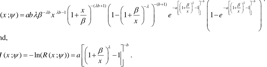
( ), skewness (Sk) and kurtosis (Ku) change for various values of parameters b, , a and, numerical values are obtained. Table 1 contains the mean, variance, Sk and Ku of the WIL distribution for various values of parameters b, , a and. It can be noticed that both the mean and variance are non-decreasing for various values of b, , a and. Also, it can be noticed that both the Sk and the Ku are decreasing for various values of b, , aand.
Table 1: Mean, variance, skewness and kurtosis of WIL distribution for various values of b, , aand
b
a=0.5 =2 a=0.5 =4.5 a=0.5 =2 a=0.5 =4.51
12 1 12 Sk Ku Sk Ku 3
2 2.186 5.694 4.918 28.827 0.452 1.692 0.452 1.692 2.5 2.842 9.524 6.395 48.215 0.428 1.650 0.428 1.650 3 3.501 14.349 7.876 72.641 0.412 1.622 0.412 1.622
3.5
2 2.202 5.552 4.954 28.105 0.354 1.508 0.354 1.508 2.5 2.862 9.304 6.440 47.101 0.334 1.477 0.334 1.477 3 3.525 14.035 7.931 71.052 0.321 1.457 0.321 1.457
4
2 2.217 5.474 4.988 27.714 0.285 1.392 0.285 1.392 2.5 2.881 9.187 0.269 46.507 0.269 1.368 0.269 1.368 3 3.548 13.869 7.983 70.214 0.258 1.353 0.258 1.353
5
Recall the Taylor’s series expansion of the function etx,that is 0 ( ) , ! s tx s tx e s =
=
so the moment generating function of the WIL distribution for |t| < 1, is given by, , , 0
(
)
(1
) (
(
))
( )
,
1,2,...,
( (
)) !
s
x i j
i j s
t
s
s
b
bi
j
M
t
w
s
b
bi
j s
= − +
+
+
=
=
+
+
The kth inverse moment, for the WIL distribution is derived by using pdf (9) as follows
, 0
1
(1
) ( (
)
)
,
1, 2,...,
( (
) 1)
k k
i j
k
b
bi
j
k
E
k
X
b
bi
j
− = +
+
+
−
=
=
+
+
+
The harmonic mean of the WIL distribution can be obtained by using the first inverse moment.
3.2. Rényi Entropy
The entropy of a random variable provides an excellent tool to quantify the amount of information (or uncertainty) contained in a random observation regarding its parent distribution (population). A large value of entropy implies the greater uncertainty in the data (Rényi, 1961). The concept of entropy is important in various situations in science, engineering and economics. The Rényi entropy of a random variable X is defined by
(
)
1 0
( ) (1 ) log ( ) ,
R
I x f x dx
−
= −
(11)for 0,and 1. The Rényi entropy of the WIL distribution is obtained by inserting the pdf (5) in (11) as follows
(
)
1 ( 1) ( 1) 1 1 ( 1) 0 1( ) log 1 1 1 .
(1 ) b x a b b x b b R x
I x ab x e dx
x − − + − − + − + − − + − − = + − + −
After simplification, the Rényi entropy of WIL can be expressed as follows
(
)
1 , 01 ( ) ( ( 1) )
( ) log ((2 1) 1, ( ) 1) .
(1 ) ( ( 1) ) !j!
j
R
i j
a b bj i
I x ab bj bi b
b bj i
− = − + + + = − + + + − + −
+ + 3.3 Distribution of Order Statistics
A closed form expression for the pdf of the uthorder statistics of the WIL distribution is
derived. Let X(1)< X(2),…, <X(n) be the order statistics for a random sample X1, X2,…, Xn
of size n from WIL distribution. It is known that, the pdf of the uth order statistic is defined by
( ) 1 0 1( ; ) ( 1) ( ; ) ( ; ).
( , 1)
u n u u p p X p n u
f x F x f x
p B u n u
− + −
=
−
= −
− +
(12)( )
( ( ) 1) ( )
1
( ) 1 , , , , ,
0 0 , , , 0
1
, , , , ,
( ; )
1
1
,
1 ( 1)
(
1
) (
)
(
1) ! ! ! (
)
u
b bi j bm h
u p n u
b bi j
X p k i j m h
p k i j m h
i k m p i m m p k i j m h
x
f
x
b x
x
n u
u
p
a
k
b bi
j
bm
h
p
k
b bi
i j m
bm
− + + + − + + − − + + − = = = + + + + +
=
+
+
−
+ −
−
+ + +
+
=
+ +
.
!
h
(13)The pdf of the smallest and largest order statistic of WIL distribution is obtained by setting u =1 and u = n in (13), respectively, as follows
(1)
( ( ) 1) ( )
1
( ) 1 , , , , ,
0 0 , , , 0
1
, , , , ,
( ; )
1
1
,
1
( 1)
(
1
) (
)
,
(
1) ! ! ! (
) !
b bi j bm h
p n
b bi j
X p k i j m h
p k i j m h
i k m p i m m p k i j m h
x
f
x
b x
x
n
p
a
k
b
bi
j
bm
h
p
k
b
bi
i j m
bm h
− + + + − + − + + − = = = + + + + +
=
+
+
−
−
+ + +
+
=
+ +
and, ( )( ( ) 1) ( )
1
( ) 1 , , , ,
0 , , , 0
1
, , , ,
( ; )
1
1
,
1 ( 1)
(
1
) (
)
.
(
1) ! ! ! (
) !
n
b bi j bm h
n p
b bi j
X k i j m h
k i j m h
i k m p i m m k i j m h
x
f
x
b x
x
u
n
a
k
b
bi
j
bm
h
k
b
bi
i j m
bm h
− + + + − + + − + + − = = + + + + +
=
+
+
+ −
−
+ + +
+
=
+ +
3.4 Quantile Function
The quantile function of X, where X~WIL
( ; )
x
is obtained by inverting XQ = F-1(Q) as1 1 1
1
ln(1 ) b 1 1 , 0< 1.
Q
X Q Q
a − − = − − + − (14)
Setting Q =0.5 in (14) gives the median of X. Simulating the WIL random variable is straightforward. If Q is a uniform variate on the unit interval (0,1), then the random variable X follows (5).
4. Estimation of the Model Parameters
In this section, ML estimators of the population parameters for WIL distribution are derived based on Type II censored samples. ML, reliability function estimators and approximate confidence interval (CI) for the population parameters are obtained.
Let n items, whose life time's follow the WIL distribution (5) are put on test. The test is terminated when the rth item fails for some fixed value of r. The lifetimes of these first r failed items, say X(1)< X(2) <…< X(r) are observed. The log likelihood function of the WIL
( )
( )
( 1)
( 1) 1 1
( ) 1 ( )
1 ( )
1 1
!
( , , , , ) 1 1 1 ( )! . b i b i b b a r x i b b i i i n r a x x n
L a b x ab x e
n r x
e − − − + − − + − + − − − = − − + − = − + − +
For simplicity, we write xiinstead of x( )i .The log likelihood function of the WIL distribution, denoted by ln ,l is obtained as follows
(
)
(
)
1 1
1 1
ln ln ! ( )! ln ln ln ln ( 1) ln( ) ( 1) ln(1 )
( 1) ln 1 1 ( ) 1 ,
r r i i i i r r b b
i i r
i i
x
l n n r r a r r b r b b x b
b E a D n r a D
= = − − = = = − + + + − + − − + + − + − − − − − −
where, i (1 ) , i (1 ) .
i i
D E
x x
−
= + = + The components of the score vector (lnl
,lnl a
, lnl b, lnl
) are obtained as follows
( 1)(
)
( 1)1
1 1 1
1 ln
ln ln ln 1 ( 1) ( 1) ln 1
1 ln 1 1 ln 1 ,
b b
r r r
i
i i
i i i i
r
i i r r
i i i
x
l r
br b x b b D
x
ba D D n r ab D D
x x − + − + − = = = = = − + − + − + − + + − + + − − +
(
)
1 1 1 1
ln
ln ln ln 1 ln 1 1 ln 1
( ) 1 ln 1 ,
r r r r
b i
i i i i
i i i i
b
r r
x
l r
r x E a D D
b b
n r a D D
− = = = = − = − + − + − − + − − + − − −
and,(
) (
) (
)
( )(
)
( ) 1 1 1 1 11 1 1
1 1 1 ln
1 1 1
(1 )
1 ,
r r r
b
i i i
i
i i i i i i i
b r
r
r
x E D
l br
b b ab D
x x E x
D
n r ab D
x + − − + = = = − − + − = + + + + + − + − + − −
The ML estimators of the unknown parameters of the WIL distribution can be obtained by solving the following non-linear equations:lnl =
0, lnl = a 0, lnl =b 0andlnl
0.For interval estimation of the parameters, the 4 4 observed information matrix ( ) { wx}
I = I for( , )w x =( , , , ), a b are obtained. Under the regularity conditions, the known asymptotic properties of the ML method ensure that:
1 4
ˆ
( ) d (0, ( ))
n − ⎯⎯→N I− asn → where⎯⎯d→ means the convergence in distribution, with mean 0=(0, 0, 0, 0)T and 4 4 covariance matrixI−1( ) then, the approximate 100(1-)% two sided CIs for
, , , ,
a b
are respectively, given by:2 2 ˆ ˆ 2
ˆ Z var( ),ˆ aˆ Z var( ),aˆ b var( ),b ˆ Z var( ).ˆ
Here, Z 2 is the upper
2thpercentile of the standard normal distribution and var (.)’s denote the diagonal elements of I−1( ) corresponding to the model parameters.
5. Simulation Study
In this section, numerical study is presented to illustrate the performance of the estimates for different parameter values and at two censoring levels. The performance of the estimates of unknown parameters and the reliability function are measured in terms of their mean square errors (MSEs), bias, standard errors (SEs), lower confidence bound (LCB), upper confidence bound (UCB), and the length of 95%, CI. The numerical procedures are defined through the following algorithm.
Step (1): 1000 random samples of size n = 50, 100 and 150 are selected; these random samples are generated from the WIL distribution.
Step (2): The number of failure items; r, based on two levels of censoring schemes, is selected at 90% and 70% censoring levels.
Step (3): Different values of the unknown parameters ( , , , a b ) are selected as as Set1≡ (=0.5,a=2,b =0.5, =0.7), Set2≡ (=0.7,a=1.8,b =0.8, =0.5), Set3≡
(=0.9,a=2.2,b=0.5, =0.7) and Set4≡ (=0.7,a=1.6,b=0.5, =0.5).
Step (4): For all sample sizes and for parameters values; the MSE, bias, and SE are computed.
Step (5): The LCB, UCB and length of CIs with confidence level 0.95 for all samples sizes and parameters values are computed.
Step (6): ML estimates and 95% CI for reliability function at the different mission time's t0 where (t0 =0.1, 0.3 and 0.6) for different sample sizes and level of censoring r =0.9n
are calculated.
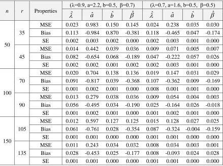
Numerical results are outlined in Tables 2 to 7. From these tables, the following observations can be detected about the performance of the estimated parameters:
▪ For all set of parameters, SE of all estimated parameters decreases as n increases. Also, the SEs for all set of parameters at censoring level 90% are smaller than the corresponding at censoring level 70% (see Tables 2 and 3).
▪ The MSEs and SEs of and are smaller than the corresponding MSEs and SEs for the other estimates for a and b in most of situations (see Tables 2 and 3).
▪ For the same sample size, for fixed value of =0.5, =0.7 and as the value of a increases, the MSE and bias of a increase (see Table 2).
▪ The length of CIs for the population parameters decreases as n increases (see Tables 4 and 5).
▪ The MSE for the Set 4 has the smallest values corresponding to other sets.
▪ The ML estimates of reliability function decrease as the mission time's increase for all values of parameters.
▪ The length of CI gets shorter when n increases (see Tables 4, 5, 6 and 7).
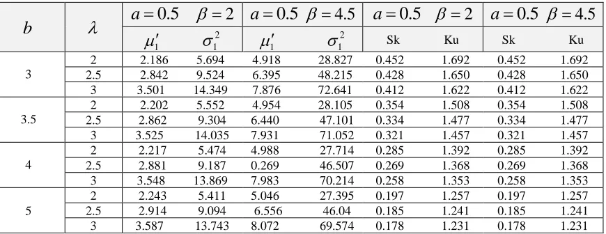
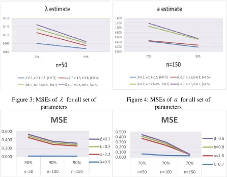
▪ The MSE of all ML estimates decreases as the censoring level increases for all sets of parameters (see for examples Figures 3 and 4).
▪ The ML estimates decrease as the censoring level increases. Also, the Set 1 has the smallest MSE compared to the other sets.
▪ The MSE of ML estimates of Set 3 at censoring level 90% decreases as n increases (see Figure 5). Also, the MSE of ML estimates of Set 2 at censoring level 70% decreases as n increases (see Figure 6).
Figure 3: MSEs of
for all set of parametersFigure 4: MSEs of a for all set of parameters
Figure 5: MSEs of Set 3 at 90% level of censoring
Figure6: MSEs of Set2 at 70% level of censoring
0.000 0.200 0.400 0.600
90% 90% 90% n=50 n=100 n=150
MSE
β=0.7
b=0.5 a=2.2
λ=0.9 0.000
0.100 0.200 0.300 0.400 0.500
70% 70% 70% n=50 n=100 n=150
MSE
β=0.5
b=0.8 a=1.8
Table 2: The MSE, bias and SE of the estimates for Set 1 and Set 2
n r Properties
(λ=0.5, a=2, b=0.5, β=0.7) (λ=0.7, a=1.8, b=0.8, β=0.5) ˆ
aˆ bˆ
ˆ
ˆ aˆ bˆ
ˆ50
35
MSE 0.051 0.632 0.268 0.265 0.064 0.307 0.042 0.034 Bias 0.207 -0.772 -0.052 -0.515 0.239 -0.547 0.002 -0.184
SE 0.002 0.004 0.001 0.000 0.002 0.002 0.002 0.000
45
MSE 0.020 0.392 0.143 0.139 0.019 0.184 0.016 0.008 Bias 0.108 -0.584 -0.022 -0.373 0.119 -0.417 0.047 -0.086
SE 0.002 0.005 0.001 0.000 0.001 0.002 0.002 0.005
100
70
MSE 0.044 0.471 0.245 0.244 0.033 0.203 0.033 0.029 Bias 0.190 -0.654 -0.078 -0.493 0.168 -0.441 -0.023 -0.167
SE 0.001 0.002 0.001 0.000 0.007 0.001 0.001 0.000
90
MSE 0.014 0.287 0.119 0.117 0.015 0.135 0.017 0.013 Bias 0.088 -0.495 -0.035 -0.341 0.096 -0.338 -0.004 -0.106
SE 0.001 0.002 0.001 0.000 0.001 0.001 0.001 0.000
150
105
MSE 0.039 0.437 0.232 0.232 0.028 0.025 0.003 0.001 Bias 0.183 -0.630 -0.083 -0.480 0.155 0.023 -0.029 0.017 SE 0.001 0.001 0.000 0.000 0.000 0.001 0.000 0.000
135
MSE 0.004 0.183 0.026 0.026 0.014 0.086 0.005 0.000 Bias 0.048 -0.387 -0.009 -0.155 0.055 -0.102 0.012 -0.005
SE 0.000 0.001 0.000 0.000 0.007 0.002 0.001 0.000
Table 3: The MSE, bias and SE of the estimates for Set 3 and Set 4
n r Properties
(λ=0.9, a=2.2, b=0.5, β=0.7) (λ=0.7, a=1.6, b=0.5, β=0.5) ˆ
aˆ bˆ
ˆ
ˆ aˆ bˆ
ˆ50 35
MSE 0.023 0.983 0.150 0.145 0.024 0.238 0.035 0.030
Bias 0.113 -0.984 0.870 -0.381 0.118 -0.465 0.047 -0.174
SE 0.002 0.003 0.002 0.000 0.002 0.003 0.001 0.000
45
MSE 0.014 0.442 0.039 0.036 0.009 0.071 0.005 0.007
Bias 0.082 -0.654 0.068 -0.189 0.047 -0.222 0.057 0.026
SE 0.002 0.002 0.001 0.002 0.002 0.003 0.001 0.000
100 70
MSE 0.020 0.704 0.138 0.136 0.019 0.147 0.031 0.029
Bias 0.091 -0.817 0.039 -0.368 0.107 -0.362 0.009 -0.169
SE 0.001 0.002 0.001 0.000 0.008 0.001 0.001 0.000
90
MSE 0.013 0.279 0.038 0.036 0.009 0.054 0.004 0.003
Bias 0.056 -0.495 0.034 -0.190 0.025 -0.164 0.026 -0.018
SE 0.001 0.002 0.001 0.000 0.001 0.002 0.001 0.000
150 105
MSE 0.012 0.597 0.127 0.125 0.015 0.128 0.027 0.025
Bias 0.061 -0.761 0.028 -0.354 0.087 -0.324 -0.004 -0.159
SE 0.001 0.001 0.000 0.000 0.001 0.001 0.000 0.000
135
MSE 0.011 0.243 0.034 0.032 0.008 0.034 0.003 0.001
Bias 0.028 -0.453 0.025 -0.177 0.008 -0.093 0.024 0.028
Table 4: LCB, UCB and Length of the estimates for Set 1 and Set 2
n r Parameters (λ=0.5, a=2, b=0.5, β=0.7) (λ=0.7, a=1.8, b=0.8, β=0.5)
LCB UCB Length LCB UCB Length
50 35
λ 0.703 0.710 0.007 0.936 0.942 0.007
a 1.221 1.236 0.015 1.250 1.258 0.008
b 0.445 0.450 0.004 0.800 0.808 0.007
β 0.185 0.448 0.263 0.315 0.805 0.490
45
λ 0.605 0.612 0.007 0.816 0.822 0.005
a 1.407 1.425 0.018 1.379 1.387 0.008
b 0.476 0.480 0.004 0.843 0.850 0.007
β 0.327 0.478 0.151 0.413 0.848 0.434
100 70
λ 0.691 0.694 0.003 0.867 0.869 0.003
a 1.338 1.346 0.008 1.459 1.465 0.006
b 0.422 0.424 0.002 0.775 0.778 0.003
β 0.211 0.423 0.212 0.333 0.777 0.445
90
λ 0.591 0.595 0.003 0.794 0.797 0.003
a 1.495 1.504 0.008 1.357 1.361 0.004
b 0.464 0.466 0.002 0.795 0.798 0.003
β 0.350 0.465 0.114 0.798 0.797 0.404
150 105
λ 0.682 0.684 0.002 0.854 0.856 0.002
a 1.367 1.372 0.005 1.821 1.825 0.004
b 0.417 0.418 0.001 0.770 0.772 0.001
β 0.219 0.417 0.198 0.517 0.771 0.300
135
λ 0.577 0.579 0.002 0.754 0.756 0.002
a 1.501 1.505 0.005 1.698 1.702 0.004
b 0.461 0.463 0.001 0.811 0.813 0.002
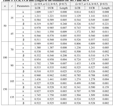
Table 5: LCB, UCB and Length of the estimates for Set 3 and Set 4
n r Parameters (λ=0.9, a=2.2, b=0.5, β=0.7) (λ=0.7, a=1.6, b=0.5, β=0.5)
LCB UCB Length LCB UCB Length
50 35
λ 1.009 1.017 0.008 0.814 0.822 0.008
a 1.211 1.221 0.010 1.129 1.141 0.012
b 0.584 0.589 0.005 0.544 0.549 0.005
β 0.319 0.587 0.268 0.326 0.547 0.221
45
λ 0.978 0.985 0.007 0.743 0.750 0.006
a 1.541 1.550 0.009 1.372 1.383 0.011
b 0.566 0.570 0.005 0.555 0.560 0.005
β 0.511 0.568 0.058 0.526 0.557 0.032
100 70
λ 0.989 0.993 0.004 0.806 0.809 0.003
a 1.380 1.387 0.008 1.236 1.241 0.005
b 0.538 0.540 0.002 0.508 0.510 0.002
β 0.332 0.540 0.208 0.331 0.510 0.179
90
λ 0.954 0.958 0.004 0.724 0.727 0.003
a 1.702 1.709 0.007 1.433 1.438 0.005
b 0.533 0.535 0.002 0.525 0.527 0.002
β 0.510 0.535 0.025 0.524 0.526 0.002
150 105
λ 0.960 0.962 0.002 0.785 0.788 0.002
a 1.436 1.441 0.005 1.274 1.278 0.004
b 0.527 0.528 0.001 0.499 0.500 0.001
β 0.346 0.528 0.182 0.341 0.500 0.159
135
λ 0.927 0.929 0.003 0.707 0.709 0.002
a 1.745 1.750 0.005 1.504 1.509 0.004
b 0.524 0.525 0.001 0.524 0.525 0.001
β 0.522 0.525 0.003 0.526 0.528 0.002
Table 6: ML estimates and 95% CI of reliability function for Set 1 and Set 2 at censoring level r =0.9 n
(λ=0.5, a=2, b=0.5, β=0.7) (λ=0.7, a=1.8, b=0.8, β=0.5)
n r t0 average
95%CI
average 95%CI
LCB UCB Length LCB UCB Length
50 45
0.1 0.972 0.948 0.996 0.048 1.000 1.000 1.000 0.000
0.3 0.803 0.765 0.840 0.075 0.998 0.997 1.000 0.003
0.6 0.510 0.473 0.548 0.075 0.972 0.959 0.985 0.026
100 90
0.1 0.995 0.994 0.996 0.002 0.996 0.986 1.007 0.022
0.3 0.729 0.711 0.747 0.036 0.996 0.983 1.008 0.024
0.6 0.518 0.498 0.537 0.038 0.981 0.968 0.995 0.026
150 135
0.1 0.995 0.994 0.996 0.002 0.998 0.992 1.004 0.012
0.3 0.721 0.707 0.735 0.028 0.998 0.991 1.005 0.014
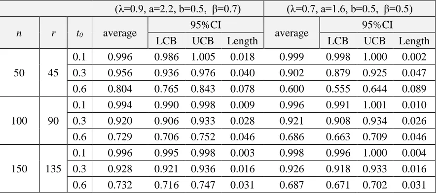
Table 7: ML estimates and 95% CI of reliability function for Set 3 and Set 4 at censoring level r =0.9 n
(λ=0.9, a=2.2, b=0.5, β=0.7) (λ=0.7, a=1.6, b=0.5, β=0.5)
n r t0 average
95%CI
average 95%CI
LCB UCB Length LCB UCB Length
50 45
0.1 0.996 0.986 1.005 0.018 0.999 0.998 1.000 0.002
0.3 0.956 0.936 0.976 0.040 0.902 0.879 0.925 0.047
0.6 0.804 0.765 0.843 0.078 0.600 0.555 0.644 0.089
100 90
0.1 0.994 0.990 0.998 0.009 0.996 0.991 1.001 0.010
0.3 0.920 0.906 0.933 0.028 0.921 0.908 0.934 0.026
0.6 0.729 0.706 0.752 0.046 0.686 0.663 0.709 0.046
150 135
0.1 0.996 0.995 0.998 0.003 0.998 0.996 1.000 0.004
0.3 0.928 0.921 0.936 0.016 0.926 0.918 0.933 0.016
0.6 0.732 0.716 0.747 0.031 0.687 0.671 0.702 0.031
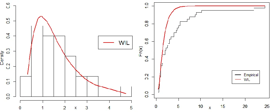
6. Applications
In this section, two real data sets are provided to illustrate the importance of the WIL distribution. The first data set refers to Hinkley (1977), which consists of thirty successive values of March precipitation (in inches) in Minneapolis/St Paul. The data are listed as follows: 0.77, 1.74, 0.81, 1.20, 1.95, 1.20, 0.47, 1.43, 3.37, 2.20, 3.00, 3.09, 1.51, 2.10, 0.52, 1.62, 1.31, 0.32, 0.59, 0.81, 2.81, 1.87, 1.18, 1.35, 4.75, 2.48, 0.96, 1.89, 0.90, 2.05
The second data refer to Jorgensen (1982) will be considered, it consists of 40 observations of the active repair times (in hours) for airborne communication transceiver. The data are: 0.50, 0.60, 0.60, 0.70, 0.70, 0.70, 0.80, 0.80, 1.00, 1.00, 1.00, 1.00, 1.10, 1.30, 1.50, 1.50, 1.50, 1.50, 2.00, 2.00, 2.20, 2.50, 2.70, 3.00, 3.00, 3.30, 4.00, 4.00, 4.50, 4.70, 5.00, 5.40 5.40, 7.00, 7.50, 8.80, 9.00, 10.20, 22.00, 24.50.
Figure 7:Estimated pdf and cdf of the WIL model for the first data
Figure 8: Estimated pdf and cdf of the WIL model for the second data Furthermore, the ML estimates of the population parameters, reliability function and their SEs for both real data sets based on TIIC are listed in Table 8.
Table 8: ML estimate of the parameters, reliability function and their SEs Based on TIIC samples
First Real Data Second Real Data n r t0 estimator estimate SEs n r t0 estimator estimate SEs
30 21 0.1
ˆ
7.59 0.27240 28 0.1
ˆ
30.71 0.913 ˆa 3.533 0.103 aˆ 1.86 0.022
ˆ
b 0.873 0.019 bˆ 0.401 0.004
ˆ
0.430 0.011 ˆ 0.176 0.004
0 ˆ ( )
7. Concluding Remarks
In this paper, a new distribution with four parameters, called the Weibull inverse Lomax distribution is introduced. Some of the statistical properties of the new distribution such as quantile function, moments, order statistics and Rényi entropy are obtained. Maximum likelihood estimators of population parameters are obtained based on Type II censored samples. The approximate confidence intervals for the model parameters and reliability function are derived. Simulation study is presented to illustrate the performance of estimates for two censoring schemes. Two real data sets are presented to illustrate theortical results.
Acknowledgements
The authors would like to thank the Editor and the anonymous referees, for their valuable and very constructive comments, which have greatly improved the contents of the paper.
References
1. Abouelmagd, T.H.M., Al-mualim, S., Elgarhy, M., Afify, A. Z., and Ahmad, M. (2017). Properties of the four-parameter Weibull distribution and its applications. Pakistan Journal of Statistics, 33(6), 449-466.
2. Alzaatreh, A., Lee, C. and Famoye, F. (2013). A new method for generating families of continuous distributions. Metron, 71, 63-79.
3. Bourguignon, M., Silva, R. B. and Cordeiro, G. M. (2014). The Weibull-G family of probability distributions. Journal of Data Science, 12, 53-68.
4. Eugene, N., Lee, C. and Famoye, F. (2002). The beta –normal distribution and its applications. Communications in Statistics–Theory and Methods, 31(4), 497-512. 5. Fisher, B. and Kılıcman, A. (2012). Some results on the gamma function for
negative integers. Applied Mathematics and Information Sciences, 6, 173-176. 6. Hassan, A. S., Elbatal, I. and Hemeda, S. E. (2016). Weibull quasi Lindley
distribution and its statistical properties with applications to lifetime data. International Journal of Applied Mathematics and Statistics, 55(3), 63-80.
7. Hinkley, D. (1977).On Quick Choice of Power Transformations. Journal of the Royal Statistical Society, Series(c), Applied Statistics, 26(1), 67–69.
8. Ibrahim, N. A, Khaleel, M. A. Merovci, F., Kilicman, A. and Shitan, M. (2017). Weibull Burr X distribution properties and application. Pakistan Journal of Statistics, 33(5), 315-336.
9. Jones, M. C. (2004). Families of distributions arising from distributions of order statistics. Test, 13, 1-43.
10. Jorgensen, B. (1982). Statistical properties of the generalized inverse Gaussian distribution, Springer-Verlag, New York.
11. Kleiber, C. (2004). Lorenz ordering of order statistics from log-logistic and related distributions. Journal of Statistical Planning and Inference, 120, 13-19. 12. Kleiber, C., and Kotz, S. (2003). Statistical size distributions in economics and
13. McKenzie, D., Miller, C., and Falk, D. A. (2011). The Landscape Ecology of Fire. Springer Dordrecht Heidelberg, New York.
14. Merovci, F. and Elbatal, I. (2015). Weibull Rayleigh distribution: theory and applications. Applied Mathematics and Information Sciences, 5(9), 1-11
15. Rahman, J., and Aslam, M. (2014). Interval prediction of future order statistics in two-component mixture inverse Lomax model: a Bayesian approach. American Journal of Mathematical and Management Science, 33, 216–227.
16. Rahman, J., and Aslam, M. (2017). On estimation of two-component mixture inverse Lomax model via Bayesian approach. International Journal of System Assurance Engineering and Management, 8, 99-109.
17. Rahman, J., Aslam, M., and Ali, S. (2013). Estimation and prediction of inverse Lomax model via Bayesian Approach. Caspian Journal of Applied Sciences Research, 2(3), 43–56.
18. Rényi A. (1961). On measures of entropy and information. In: Proceedings of the 4th Fourth Berkeley Symposium on Mathematical Statistics and Probability, 547-561. University of California Press, Berkeley
19. Reyad, H. M., and Othman, S. A. (2018). E- Bayesian estimation of two- component mixture of inverse Lomax distribution based on type- I censoring scheme, Journal of Advances in Mathematics and Computer Science (26) 2, 1-22. 20. Singh, S. K., Singh, U. and Yadav, A. S. (2016). Reliability estimation for inverse
Lomax distribution under type Π censored data using Markov chain Monte Carlo method. International Journal of Mathematics and Statistics, 17(1), 128-146. 21. Tahir, M. H., Cordeiro, G. M., Mansoor, M. and Zubair, M., (2015). The
Weibull-Lomax distribution: properties and applications. Hacettepe Journal of Mathematics and Statistics, 44 (2), 461 – 480