Application of optical tomography in the study of discolouration in drinking water distribution systems

Drink. Water Eng. Sci., 4, 61–69, 2011 www.drink-water-eng-sci.net/4/61/2011/ doi:10.5194/dwes-4-61-2011

©Author(s) 2011. CC Attribution 3.0 License.

History

of

Geo- and Space

Sciences

Open

Access

Advances

in

Science & Research

Open Access Proceedings

Drinking Water

Open Access Open Access

Earth System

Science

Data

Drinking Water

Discussions O pen Acc es s Open Access

Earth System

Science

Data

Application of optical tomography in the study of

discolouration in drinking water distribution systems

P. van Thienen, R. Floris, and S. Meijering

KWR Watercycle Research Institute, P.O. Box 1072, 3430 BB Nieuwegein, The Netherlands

Received: 10 May 2011 – Published in Drink. Water Eng. Sci. Discuss.: 27 June 2011 Revised: 7 November 2011 – Accepted: 20 November 2011 – Published: 7 December 2011

Abstract. Theories describing the turbulent deposition of particles from aerosols have recently been applied to

drinking water distribution. In order to allow the study of these processes in a quantitative way and internally observe a cloud of suspended particles in a pipe, we have developed an optical tomography technique and measuring device using low cost electronic components specifically for this application. The mathematical methodology and the electronic device are described in this paper, and tests of both the mathematical approach and the actual device are presented. We conclude that the mathematical framework presented is suitable and that the technical implementation works in a test setting. The described methodology may provide a valuable tool for the study of processes related to drinking water discolouration in the lab.

1 Introduction

Water discolouration continues to be one of the prime rea-sons for customer complaints relating to water quality to be received by water companies (Husband and Boxall, 2011). The resuspension of particles present in the drinking water distribution system by a hydraulic disturbance is usually in-voked to explain its occurrence (Vreeburg and Boxall, 2007). A chain of events or processes can be identified in the gener-ation of a discolourgener-ation event, i.e. origin, evolution,

deposi-tion, cohesion/adhesion and resuspension of particles.

The suggestion that currently applied models do not en-compass the complete range of physical processes respon-sible for the occurrence of discolouration (Blokker et al., 2010) has led van Thienen and Vreeburg (2010) and van Thienen et al. (2011b) to theoretically investigate the

possi-bility of processes other than gravitational settling affecting

particle deposition. Their findings predict the occurrence of the turbulent process of turbophoresis under specific condi-tions which may be expected in transport mains. In order to experimentally verify these predictions, a method of inter-nally observing a pipe in which this process is supposed to take place is required. In this paper, the required methodol-ogy, of which a preview has been presented by van Thienen et al. (2011a), is developed using the principles of optical

Correspondence to: P. van Thienen

([email protected])

tomography. The method allows its user to study particle transport, deposition and resuspension behaviour in a

trans-parent pipe both qualitatively (in terms of different structures

in the particle concentration field relating to different

mecha-nisms) and quantitatively (in terms of radial transport veloci-ties). The technique uses a sophisticated inversion scheme to

include and deal with the effects of measurement

uncertain-ties and noise.

Tomography is a well established technology in the field of medicine (see e.g. Bibb and Winder, 2010), allowing doctors a non-destructive view inside a patient. It is also used e.g. in geophysics to view inside the Earth using seismic waves (e.g. Bijwaard and Spakman, 1999), and has been applied to industrial gravity chutes (Zheng et al., 2006). However, its application in drinking water research is new.

2 Methodology

2.1 Principle

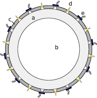
Fig. 1.Schematic set-up of the measurement device. The image shows a cross section of the perspex pipe (a) filled with water (b). A tightly fitting PVC ring (c) is fitted around the pipe. Tapered holes have been drilled in this ring, into which alternating LEDs (d) and light sensors (e) have been placed.

figure

16

Figure 1.Schematic set-up of the measurement device. The image shows a cross section of the perspex pipe (a) filled with water (b). A tightly fitting PVC ring (c) is fitted around the pipe. Tapered holes have been drilled in this ring, into which alternating LEDs (d) and light sensors (e) have been placed.

combining these measurements, a clear image of the cross-sectional particle concentration field can be obtained.

2.2 Measuring device set-up

A PVC ring containing ten evenly spaced LEDs with ten evenly spaced sensors in-between is fixed around the trans-parent tube (see Fig. 1). The LEDs are high-power white LEDs; the sensors are Phidget light sensors (Phidgets, 2010). An Arduino Mega micro-controller (Arduino, 2010) with custom software is used to control the LEDs (using switch-ing electronics) and also contains the AD-converters which are used to digitally read the light sensors (10 bit resolu-tion). The Arduino board is connected to a computer using a USB cable. At regular intervals (typically a few seconds), the LEDs are briefly switched on successively. While a sin-gle LED is illuminated, all light sensors are read. This entire measurement cycle takes only a fraction of a second. When all sensor readings have been collected, they are sent to the computer for processing. We note that the measuring device was constructed exclusively from low cost components.

2.3 Refraction and reflection

Because of significantly different optical densities, light is

re-fracted and reflected both at the air-perspex interfaces and at the perspex-water interfaces. The Fresnel equations (see e.g. Brass, 2010) allow the calculation of the relative amounts of light which are reflected and refracted. Snell’s law sub-sequently provides the angle of refraction. Based on these

cases (Fig. 2b–e), however, show that most light reaching the sensors follows the most direct route through the pipe, i.e. by subsequent refraction at the air-perspex, perspex-water, opposite water-perspex, and opposite perspex-air transitions, which is generally close to the imaginary line connecting LED and sensor.

2.4 Mathematical description 2.4.1 Physical assumptions

In the following, a number of assumptions will be made. These are:

– The fraction of light which is scattered by suspended

particles increases in some way with the particle con-centration. As a result, the relative amount of light which passes through the suspension decreases with in-creasing particle concentration.

– A simple optical model is used in which particles only

cast shadows and their concentration is sufficiently low

for particles not to be in each other’s shadows. No

scat-tering or reflection of light offparticles is taken into

ac-count.

2.4.2 Model set-up

The cross-sectional domain is discretized into a number of triangles. On the corners of each of these triangles, an

(ini-tially unknown) light absorption coefficient is defined. For

each light beam (path from LED to light sensor), an equation can be written which describes the decrease in intensity of the light beam as a function of the (unknown) light

absorp-tion coefficients. The relative light intensity decrease can be

written as the ratio of the intensity decrease to the reference intensity:

(IE−IR)

IE

!

= Σn

j=1

Z

path

c(l)dl (1)

In this expression, IEis the unperturbed or reference light

intensity at the receiver and IR is the measured light

inten-sity at the receiver in the perturbed experimental situation. A summation is made over all n elements in the

(a) (b) (c)

(d) (e)

Fig. 2. Light paths from a single LED (top of graphs) to five sensors (a-e; the other five sensors are their mirror images), including refraction and reflection (up to 7 times). Colours indicate beam intensity relative to emission, ranging from green (0.001) to pink (0.1), with black segments indicating a relative intensity of less than 0.001.

17

Figure 2. Light paths from a single LED (top of graphs) to five sensors (a–e; the other five sensors are their mirror images), including refraction and reflection (up to 7 times). Colours indicate beam intensity relative to emission, ranging from green (0.001) to pink (0.1), with black segments indicating a relative intensity of less than 0.001.

c are integrated over the path of the light beam inside each

of the elements it passes through. Combining all

measure-ments ((IE−IR)/IE)i in a vector r, all unknown absorption

coefficients c in a vector s, and all integration coefficients in

a matrix A, we get a system of equations:

As=r (2)

Solving this system of equations is an inverse problem.

2.5 Light beam paths

As indicated in Sect. 2.3, light reaches the sensors through a complex set of paths which contribute in varying amounts to the total signal. However, in most cases, 98 % or more of the light which reaches a sensor arrives through a direct path without reflections. Therefore, a simple approximation of this set of paths, a straight line connecting a LED to a beam, can be applied instead. In the following, we apply both this simple approximation (single beam model) and a full set of light paths (multiple beam model).

2.5.1 Inversion procedure

When the number of beams is equal to the number of

un-known coefficients, in principle we have a determined

sys-tem of equations, which can possibly be solved. This would

result in knowing the values of the light absorption coeffi

-cients in all nodes of the discretization, which are a proxy for the local particle concentration. However, measurement and discretization errors dominate the result if this proce-dure is applied. In addition to this, refraction and inciden-tal low beam intensities reduce the number of beams which can actually be used, resulting in a underdetermined prob-lem. A more refined inversion procedure is required to get meaningful results. Suitable methods have been developed and applied in fields in which inversion is done of mea-surements of “natural experiments” which are not controlled by the researcher, specifically geophysics (e.g. Bijwaard and Spakman, 1999; Fokker et al., 2010). These generally suf-fer both from being underdetermined and having significant measurement uncertainties. Applying these methods (Taran-tola, 2005; Muntendam-Bos et al., 2008), the system (Eq. 2) is rewritten as:

s=CmAT(ACmAT+Cd)−1r (3)

In this expression, Cmis the covariance matrix of the prior

model matrix. It is produced by computing the covariance matrix for a large number of plausible models which span the parameter space of expected results, and contains all prior

knowledge, uncertainties and variations of the model. Cdis

(h)

(i)

(j)

(k)

(l)

(m)

(n)

(o)

(p)

(q)

(r)

(s)

(t)

(u)

(v)

Fig. 3.

Resolution and resolvability as a function of ray coverage for the single beam model. a) Domain

discretization; b) synthetic absorption coefficient field; c-g) set of beam paths used; h-l) simulated

to-mograms for these beam path sets; m-q) corresponding resolution matrices (note that SigmaT indicates

the sum of the main diagonal of the resolution matrix); r-v) posterior model variance for all degrees of

freedom. Note that frames b and h-l all use the same colour scale.

18

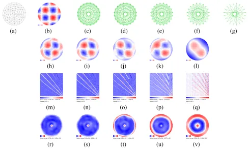
Figure 3.Resolution and resolvability as a function of ray coverage for the single beam model. (a) Domain discretization; (b) synthetic

ab-sorption coefficient field; (c–g) set of beam paths used; (h–l) simulated tomograms for these beam path sets; (m–q) corresponding resolution

matrices (note that SigmaT indicates the sum of the main diagonal of the resolution matrix); (r–v) posterior model variance for all degrees of freedom. Note that frames (b) and (h–l) all use the same colour scale.

of the measurements on the main diagonal and zeros offthe

main diagonal. The total variances consist of the actual

mea-surement variancesσ2_{mi j} which are obtained for each

LED-sensor combination ij from multiple samples which are taken

and a system varianceσ2s which is assumed to be the same

for all measurements and includes all errors which are not

included inσ2m. A representative value ofσsis chosen. The

variances are summed following Bienaym´e’s formula:

σ2

i j=σ

2 mi j+σ

2

s (4)

2.5.2 Resolution and covariance

In order to understand what quality of results can be ex-pected from the inversion procedure, we compute the resolu-tion matrix and compare prior and posterior covariance ma-trices. The resolution matrix is defined as (Tarantola, 2005; Muntendam-Bos et al., 2008):

R=CmAT(ACmAT+Cd)−1A (5)

For a perfectly resolved system, the resolution matrix is equal to the identity matrix.

The posterior covariance matrix can be computed from the resolution matrix (Tarantola, 2005; Muntendam-Bos et al., 2008):

C=(I−R)Cm (6)

This expression shows that a well-resolved posterior model with low variances is obtained for a model which has a resolution matrix close to the identity matrix. Also, it is clear from Eq. (6) that uncertainties in the prior model di-rectly propagate into the posterior model. The magnitude of this propagation depends on the resolution. For a resolved system, posterior variances should be smaller than prior vari-ances.

We shall use matrices R and C to evaluate the mathemati-cal quality of the results of the inversion procedure.

3 Tests

3.1 Mathematical approach

(a)

(b)

(c)

(d)

(e)

(f)

(g)

(h)

(i)

(j)

(k)

(l)

(m)

(n)

(o)

(p)

(q)

(r)

(s)

(t)

(u)

(v)

Fig. 4.

Resolution and resolvability as a function of ray coverage for multiple beam model. Frame

descriptions are the same as in Figure 3

19

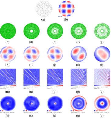
Figure 4.Resolution and resolvability as a function of ray coverage for multiple beam model. Frame descriptions are the same as in Fig. 3.

(see Sect. 2.5). Figure 4 does the same for a multiple beam model as described in Sect. 2.3. A synthetic light

absorp-tion coefficient field was generated exhibiting a checkerboard

pattern (see Figs. 3b and 4b). Corresponding synthetic mea-surements were computed for all beams based on this pat-tern (10 samples per beam), adding white noise to the mea-surements with a maximum amplitude of 10 %. These syn-thetic measurements were fed into the inversion procedure, assuming all uncertainty to originate from the measurement

error (Eq. 4,σs=0). For different beam sets displayed in

Fig. 3c–g, this results in the corresponding tomograms of Fig. 3h–l for the single beam model and Fig. 4h–l for the multiple beam model. Traditionally, checkerboard tests have often been used to illustrate the quality (or lack thereof) of an inversion procedure (e.g. Morgan et al., 2002). In the tomo-grams of Figs. 3h–l and 4h–l, a decreasing correspondence

with the original synthetic input field (Figs. 3b/4b) can be

observed for decreasing beam coverage. However, in frames

h, i and j (Figs. 3 and 4), the reconstructed image is still ac-ceptably close. An alternative, more quantitative way of de-termining the quality of the tomograms is by means of the resolution and posterior covariance matrices, as defined in Sect. 2.5.2. As has been indicated above, a resolution matrix is close to the identity matrix for a well resolved model. The sum of the main diagonal of this model indicates how many degrees of freedom are resolved. Figures 3m–q and 4m–q

show the resolution matrix for our five different beam

c to g (Table 1 and Figs. 3 and 4) – the variance reduction does decrease, however. The numbers shown in Table 1 do not show a monotonously decreasing series for the multiple beam model. This is due to the fact that all numbers are based on simulations with a significant amount of random noise in the input. As a result, all numbers presented are valid for

a single simulation but will be somewhat different when the

simulation is repeated. However, the presented set of results does illustrate a clear trend.

3.2 Inversion results

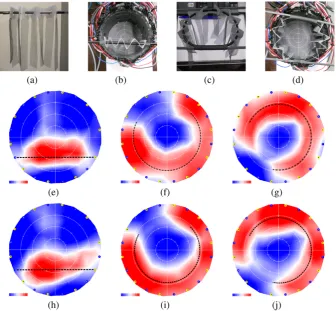
Now that the theoretical resolvability and resolution have been ascertained, lab tests are required, in which an object representative of a particle cloud is placed inside the device and located using the device. For this purpose, a curtain was made from wire mesh, which is expected to have optical properties similar to that of a cloud of dark, non-reflecting particles suspended in water and can be easily positioned side the device (see Fig. 5a, c). This curtain was placed

in-side the device in different configurations and orientations

(Fig. 5b, d). The resulting images are shown in Fig. 5e–g for the single beam model and in Fig. 5h–j for the multiple beam

model, for curtain configurations/orientations indicated by a

dashed line (note that the actual area occupied by the curtain is wider than the dashed line). The following can be said for all three cases e–g (Fig. 5) as well as for cases h–j (Fig. 5):

– The curtain is well resolved in the tomograms.

– The image of the curtain is somewhat wider than the

actual curtain.

– The ends of the curtain are not so accurately resolved.

The width can be partially explained from the limited reso-lution of the tomogram (12 elements in its diameter). The ends of the curved curtain in Fig. 5f–g and h–j may be re-lated to the fact that we are imaging an object consisting of lamellae of wire mesh, the visibility of which strongly

de-pends on their orientation relative to the different light beams

which are used in its reconstruction in the tomogram. The fact that the linear curtain in Fig. 5e does not appear to touch the walls is a resolution issue. As can be seen in Figs. 3t and 4t, the posterior model variance at the pipe wall is rather

large, meaning that this region is not well resolved. This is due to the lack of usable light beams shining more or less parallel to the wall in this region (Fig. 3e). In the case of the multiple beam model, Fig. 3e does show significant beam coverage close to the wall. However, the amount of light car-ried by these beams is so small that they contribute little to the final tomogram.

In addition to these dry tests, wet tests have been per-formed with the tomography device fitted to a vertical piece

of perspex pipe filled with water. Small amounts of coffee

granules were dropped in the water by hand in different

pat-terns, forming a sinking column of coffee particle suspension

when dropped in a single location or a wider cloud when dropped over a larger area. Working in this way, it was dif-ficult to control the exact location and shape of the particle clouds sinking through the beam field of the measurement device. However, the resulting tomograms were consistently in agreement with the visually observed locations of the par-ticle columns and clouds.

4 Discussion

4.1 Functioning

Both the mathematical consideration of the resolution of the inversion results and the dry tests which have been performed show that the device functions as intended. Also, it is capa-ble of resolving particle concentration variations in the inside of a moving body of water which can not be determined by direct observation from the outside. The more complex and computation time consuming multiple beam model does not appear to result in significantly better images than the single

beam model, but it does have a better formal resolution close

to the wall when ray coverage is reduced.

4.2 Practical considerations

During the test phase of the device, several practical issues were come across and resolved. These include the following:

– Because the variations in light intensity which are the

the shielding is incomplete, recalibration is required whenever the lighting conditions in the lab change,

re-setting IEin expression (Eq. 1).

– The optical properties of the particles are important in

the sense that highly reflective and/or scattering

parti-cles reduce the quality of the inversion results, since

re-flection and scattering offthe particles are not included

in the simple optical model which is applied. For this reason, a test material was selected which is dull and dark.

4.3 Particle concentrations

In the above, tomograms are obtained which show the

distri-bution of a “light absorption coefficient” throughout a

cross-section. This is very useful when one wants to study

con-centration differences, but the actual concentration values are

not obtained. In order to convert absorption coefficients to

concentrations, a calibration curve needs to be constructed from experiments with known particle concentrations. It is

expected that different curves are obtained for different

ma-terials with different optical surface properties.

4.4 Applications

The intended operating environment for the method which has been described in this paper is in the lab. Under nor-mal conditions, the particle concentration in drinking water is much too low to be detectable with the present optical set-up, except when hydraulic disturbances cause discolouration. In the lab, it is possible and often desirable to work with par-ticle concentrations which are much higher than in drinking water distribution systems to facilitate observation and re-duce time scales of e.g. accumulation. The first investigation in which this technique has been applied is the experimental verification of a theoretical mechanism map for turbulent par-ticle deposition in drinking water distribution systems (Floris et al., 2011). This presents results describing the conditions of initiation of particle deposition by turbophoresis, building on theoretical predictions by van Thienen et al. (2011b). A number of additional research areas in drinking water distri-bution in which the method can be applied can be thought of, such as particle resuspension, saltation and bed transport.

4.5 Limitations and possible improvements

Some limitations of the current setup are:

– Since we are considering a moving body of water, we

may expect the plug of water to advance by some dis-tance in the course of the measurement cycle. The re-sulting image is therefore only meaningful if variations in the particle concentration field do not occur on this

time and length scale. At typical flow velocities of

0.01 to 1 m s−1_{and measurement cycle times}

(depend-ing primarily on the number of samples taken) of 300 to 1500 ms, the length of the imaged plug is 3 mm to 1.5 m.

– The resolution of the tomograms is limited by the

num-ber of LEDs and sensors which have been installed.

Several improvements can be made to the device and

pro-cedure. We list the most obvious and effective:

– One of the main issues with the current setup is the

re-duced ray coverage close to the pipe wall due to the ef-fects of refraction. By proper shaping of the outside of

the transparent pipe or by choosing a different material

with a lower refractive index, this effect can be reduced.

For the latter option, however, the choice of alternative materials is not obvious, since the refractive index of perspex is already relatively low.

– Because of the time required to take all measurements,

which may add up to hundreds of milliseconds, the im-age obtained is to some degree an averim-age of the sit-uation over this time period. Using faster electronics would allow a reduction of the measurement time and thus a representation which is closer to a “real” snap-shot.

– A more sophisticated optical model including light

scat-tering (and possibly reflection) by particles should in-crease the accuracy of the tomograms and allow the use of a wider range of particle materials. This would al-leviate the following limitations of the current optical model: (1) in the current model, when particles which

do significantly scatter and/or reflect light are studied,

more light from a single source reaches all light sen-sors in varying amounts, depending on the particle dis-tribution. The method tries to explain this in terms of the applied model, i.e. a smaller amount of light being blocked by particles on the modeled beam paths, mean-ing fewer particles in these paths. (2) When high parti-cle concentrations are used, partiparti-cles start to be in each other’s shadows, more so on longer beam paths than on shorter paths. This results in a smaller amount of light intensity reduction for long beams (through the centre of the domain) per particle than for shorter beams (along the wall). As the optical model assumes equal light blocking for each particle regardless of the concentra-tion, a uniform actual particle concentration throughout the domain would result in a tomogram with a

some-what higher light absorption coefficient along the walls

than in the center.

– Finally, the resolution of the obtained images can be

in-creased by increasing the number of light paths through

Figure 5.Dry test results of the optical tomography device. (a) Linear wire mesh curtain used to represent a particle cloud; (b) positioning of the linear curtain; (c) curved wire mesh curtain; (d) positioning of the curved curtain; (e) inversion result for linear curtain (single beam path); (f, g) inversion results for curved curtain (single beam path), (h) inversion result for linear curtain (multiple beam paths); (i, j) inversion results for curved curtain (multiple beam paths). A dashed line indicates the actual position of the curtain in (e–g).

5 Conclusions

A method for studying particle processes in situ has been presented and tested. The following can be concluded:

– The mathematical framework presented here is suitable

for obtaining meaningful images from light measure-ments.

– The technical implementation is capable of resolving

semi-transparent objects in a test setting.

The presented methodology provides a useful and promis-ing technique for the study of several areas in drinkpromis-ing water discolouration research. The first application of the device and methodology is presented in Floris et al. (2011).

Acknowledgements. We thank Karin van Thienen-Visser for help with the inversion procedure, Melanie Tankerville for reviewing the English of this paper, and Mirjam Blokker and two anonymous referees for helpful comments on the manuscript.

Edited by: J. Verberk

References

Arduino: http://www.arduino.cc, last access: 6 December 2010.

Bibb, R. and Winder, J.: A review of the issues surrounding three-dimensional computed tomography for medical modelling using rapid prototyping techniques, Radiography, 16, 78–83, 2010. Bijwaard, H. and Spakman, W.: Tomographic evidence for a narrow

whole mantle plume below Iceland, Earth Planet. Sc. Lett., 266, 121–126, 1999.

Blokker, E., Vreeburg, J., Schaap, P., and van Dijk, J.: The self-cleaning velocity in practice, in: Water Distribution System Analysis conference, Tucson, Arizona, 2010.

Brass, M. E.: Handbook of Optics. Volume I: Geometrical and Physical Optics, Polarized Light, Components and Instruments, McGraw-Hill, third edn., 2010.

Floris, R. and van Thienen, P.: Experimental investigation of tur-bulent particle radial transport processes in DWDS using op-tical tomography, Drink. Water Eng. Sci. Discuss., 4, 61–83,

doi:10.5194/dwesd-4-61-2011, 2011.

Husband, P. S. and Boxall, J. B.: Asset deterioration and discoloura-tion in water distribudiscoloura-tion systems, Water Res., 45, 113–124, 2011.

Morgan, J. V., Christeson, G. L., and Zelt, C. A.: Testing the res-olution of a 3D velocity tomogram across the Chicxulub crater, Tectonophysics, 355, 215–226, 2002.

Muntendam-Bos, A. G., Kroon, I. C., and Fokker, P. A.: Time-dependent Inversion of Surface Subsidence due to Dy-namic Reservoir Compaction, Math. Geosci., 40, 159–177,

doi:10.1007/s11004-007-9135-3, 2008.

Phidgets: http://www.phidgets.com, last access: 6 December 2010.

Tarantola, A.: Inverse Problem Theory and Methods for Model Pa-rameter Estimation, Society for Industrial and Applied Mathe-matics, Philadelphia, 2005.

van Thienen, P. and Vreeburg, J.: Turbulent processes in drinking water distribution, in: Water Distribution System Analysis con-ference, Tucson, Arizona, 2010.

van Thienen, P., Floris, R., Vreeburg, J. H. G., and Blokker, E. J. M.: Lab experiments on turbulent processes causing discolouration potential, in: Proceedings of the World Environmental and Water Resources Congress, Palm Springs, California, 2011a.

van Thienen, P., Vreeburg, J., and Blokker, E.: Radial transport processes as a precursor to particle deposition in drinking water distribution systems, Water Res., 45, 1807–1818, 2011b. Vreeburg, J. and Boxall, J.: Discolouration in potable water

distri-bution systems: A review, Water Res., 41, 519–529, 2007. Zheng, Y., Liu, Q., Li, Y., and Gindy, N.: Investigation on