Comparison of Some Suggested Estimators Based on Differencing Technique in the Partial Linear Model Using Simulation

Baghdad Science Journal

Vol.16(4) 2019

DOI:http://dx.doi.org/10.21123/bsj.2019.16.4.0918

Comparison of Some Suggested Estimators Based on Differencing Technique in

the Partial Linear Model Using Simulation

Saja Mohammad Hussein

Received 15/11/2018, Accepted 28/4/2019, Published 1/12/2019

This work is licensed under a Creative Commons Attribution 4.0 International License.

Abstract:

In this paper new methods were presented based on technique of differences which is the difference- based modified jackknifed generalized ridge regression estimator(DMJGR) and difference-based generalized jackknifed ridge regression estimator(DGJR), in estimating the parameters of linear part of the partially linear model. As for the nonlinear part represented by the nonparametric function, it was estimated using Nadaraya Watson smoother. The partially linear model was compared using these proposed methods with other estimators based on differencing technique through the MSE comparisoncriterion in simulation study.

Key words: DAUGRR, DGJR, DGRR, Differences technique, DMJGR, NW estimator

Introduction:

For the following partially linear model:

)

1

...(

,...,

2

,

1

,

)

(

t

i

n

f

x

y

_i



_i







_i





_i



i y

is an nx1 vector of responses

) ,... ,

( 1 2 



 _{i i ip}

i x x x

x is an known p-dimensional

vectors,



(



₁,



₂,...



_p)is an unknown

parameter vector, f(.) is an unknown smooth function, ti are the values of the variable which the

dependent variable yi are observed ,



_i's are

independent and identically distributed random

variables with E(



i )=0 and cov(



i)=

2



_.

The partially linear model has parametric and nonparametric components; this model is more flexible than the linear model. There are a lot of studies that are interested in estimating the linear part represented by,



and the non-linear part represented by nonparametric function f (



). In this paper we focused on the technique of differences to estimate the parameters of the linear part of the partially linear model. This technique depends on the removal of the effect of the nonparametric function by differencing the data, and then estimates the linear part of the model (1) which can remove the effect of bias resulting from the existence of the nonparametric function. This technique has been used in many researches mentioning them, a vector of



was estimated using the difference method(1) Department of Statistics, College of Administration and Economics, University of Baghdad, Iraq

E-mail: [email protected]

In the partially linear model and Higher-order differences were applied using a special class of differences sequences(2) to estimate the linear part. Once a



has become known, f() can be estimated by any method of nonparametric. In the linear part of the model (1) it is usually assumed that the regressors are independent however, in practice this cannot be achieved since there is a linear or close relationship between explanatory variables, i.e. , the problem of multicollinearty, and with this problem the (OLS) method does not produce accurate and moral results, and the variances are large and far from the truth. To solve the problem of multicollinearty in the linear part of model (1), there are several methods referred to in literatures that began through the famous ridge regression estimator (3, 4). Hence, researchers assumed many estimators that address the problem of multicollinearty, which are either addition or expansion on the ridge regression estimator or they proposed other new estimators.

Among the most important studies interested in using the technique of differences to estimate the parameters of the linear part, which suffers from the problem of multicollinearty in partially linear model, which enables the researcher to see them, are:

compared with difference-based estimator



ˆ_diff by

using MSE criterion. The properties of each of difference-based ridge estimator and Liu type estimator for the partially linear semiparametric model were studied when the errors are independent with equal variance and compared the two estimators through MSE and were extended the results to errors which have the problems of heterogeneity and autocorrelation(7). Also new estimates of shrinkage parameter in generalized difference-based ridge estimator(8) were proposed for semiparametric regression model, then the risk function of the estimator was calculated and the generalized difference -based estimator was introduced to the vector of parameters



of semiparametric regression model when errors are correlated(9) and suggested the generalized restricted difference- based Liu estimator when there is a non stochastic constraint. A difference - based almost unbiased Liu estimator (DBAULE)(10), was proposed to estimate the linear part in a partial linear model, and studied its characteristics andthe generalized difference-based ridge estimator was proposed to the vector of parameters



in a partial linear model when the errors are dependent(11) and was compared the performance of proposed estimator with the generalized restricted difference-based ridge estimator by using MSE criterion. Also a Jackknifed difference- based ridge estimator (12) was proposed in partial model; the proposed estimate was compared with difference- based ridge estimator and difference- based estimator through MSE and a MSE matrix. A restricted difference- based ridge estimator(13) was suggested to the semiparametric partial linear regression model, the necessary and sufficient conditions were also derived for a new estimator to exceed the restricted least square for selecting the ridge parameter .The generalized difference -based almost unbiased ridge estimator under the constraint r = RB + e was defined and was suggested generalized difference- based on weighted mixed almost unbiased ridge estimator, and compared the performance of this estimate with the generalized difference- based weighted mixed estimator, the generalized difference -based estimator, and the generalized difference-based almost unbiased ridge estimator through MSE criterion(14). A set of differences-based estimators were presented and was suggested difference-based modified jackknifed ordinary ridge estimator(15) for estimating the parametric component of semiparametric regression model . The achievement of this estimate was compared with difference- based estimator and difference- based ridge estimator by the criterions MSE and a BIAS. The

generalized difference-based mixed Liu estimator(16) when the parameter of regression is constrained to a stochastic linear restricted was presented in the partially linear model.

The remainder of the paper is organized as follows: In the second and third sections the differencebased generalized ridge and difference -based almost unbiased generalized ridge estimator are presented, in sections 4,5 the proposed methods that based to the differences technique are presented. In section 6, biased ridge parameters used with the estimation methods are presented. As for the seventh and eighth sections the method of non-parametric estimation and cross validation are presented. In the ninth section the simulation study is presented. The final section presents the main results and conclusions of the research.

Difference-based Generalized Ridge Regression Estimator (DGRR)

In this study, the explanatory variables in Model (1) suffer from the problem of multicollinearty, and to address this problem, it was suggested adding ridge parameter (k)(3,4), a small positive amount to the elements of the diameter of the information matrix(X'X). If the ridge parameter (k) is constant for all elements of diameter , the estimator is called ordinary ridge regression (ORR), if the ridge parameter (k) is variable for all elements of diameter of information

matrix

(

X

'

X

)

,i.e.

p i

p k k k k

k k k diag

K  ( ₁, ₂,... ), 0, ₁ ₂ ... ,

the estimator is called generalized ridge regression(GRR). A difference-based generalized ridge regression estimator (DGRR)(8) was introduced using the same differences technique (1,17) in estimating vector parameters



, where it begins by removing the nonparametric part of model (1 )by multiplying it with a matrix of differences D as follows:

) 2 ...( )

( 

 Df t D Dx

Dy  

Where D(n-m)x n: represents the difference matrix and its components as follows:

        

 

        

 



m m m

m

d d

d d

d d

d d

d

D

. . 0 0 . . . 0 0

0 . . 0 . . . 0 0

. . . . . . . . . . .

. . . . . . . . . . .

. . . . . . . . . . .

0 . . . 0 .

. . 0

0 . . . 0 0 . .

0 0 0

1 0

Where m is the order of differenceing and d0,d1,…dm is the differencing weights that achieve

the following:

S.t:



0 &



2 1 j

j d

Since the data have been arranged so that the data of the nonparametric variable are close, the application of the D-matrix will lead to the elimination of the nonparametric effect. Thus, the model will become as follows:

𝑦̃ = 𝑋̃𝛽 + 𝜀̃ …(3)

Where; 𝑦̃ = 𝐷𝑦is an (n-m)x 1 vector of responses, 𝑥̃ = 𝐷𝑋 is an (n-m)x p matrix of explanatory variables.



:is an px1 vector of unknown parameters,𝜀̃ = 𝐷𝜀: is an (n-m)x 1 vector of random errors.

The vector



of model (3), which suffers from the problem of multicollinearity in its explanatory variables, is estimate by difference-based generalized ridge regression estimator (DGRR) in the following steps(8):

For the semi-positive definite matrix (X~'X~),there exists an orthogonal matrix



such that

  

(X~'X~) , : the matrix of the eigen values of(X~'X~), i.e. diag(



₁,...,



_p) .The model (3)

becomes as follows:

) 4 ...( , x ~ z , ~

~_yz



_



_{where  }



_



The difference-based generalized ridge regression estimator (DGRR) in the canonical form is as follows: ) 5 ...( ) ( ˆ ) ( ~ ) ( ˆ 1 1 K A where KA I y z K z z DOLS DGRR             

Where



ˆDOLS_{:the simple differencing based} estimator for parameter



, ˆDOLS (zz) z~y

1    



) 6 ...( ˆ ˆ DGRR DGRR







In order to calculate the parameter



in the

model(1), the modified



2 estimator is used as follows: ) 7 ...( ] ) ( [ ) ( ) ( 2 D P I D tr Dy P I Dy D     



Where, PDx[(Dx)(Dx)]1(Dx)is an (n-m) x (n-m) projection matrix

The characteristics of this estimate are:

) 11 ...( ) ( ) ( ˆ ) ( ) ( ˆ ) ˆ ( ) 10 ...( ) ( ) ( ˆ ) ˆ var( ) ) ˆ ( ))( ˆ ( ( ) ˆ var( ) ˆ ( 3 ) 9 ...( ) ˆ ( ) ˆ ( 2 ) 8 ...( ) ( ) ˆ ( 1 2 2 2 2 2 1 1 1 1 1 2 1 1 1 2 1 1







_                                     i i i i i i i DGRR DGRR DGRR DGRR DGRR DGRR DGRR DGRR DGRR k k k K A KA KA I KA I MSE KA I KA I Bias Bias MSE KA E Bias KA I E                     

Difference-based Almost Unbiased Generalized Ridge Regression Estimator (DAUGRR)

A difference-based almost unbiased generalized ridge estimator(DAUGRR)(14) was defined as follows:

)

14

...(

ˆ

ˆ

)

13

...(

ˆ

]

)

)

(

(

[

)

12

...(

ˆ

)

)

(

(

ˆ

2 1 1 DAUGRR DAUGRR DOLS DGRR DAUGRR

K

K

I

K

K

I































 

The characteristics of this estimate are:

) 18 ...( ) ( ) ( ˆ ) ˆ ( ) ( ) 17 ...( ) ( ) ( ˆ ) ˆ var( ) ) ˆ ( ( )) ˆ ( ( ) ˆ var( ) ˆ ( 3 ) 16 ...( ) ( ) ˆ ( ) ˆ ( 2 ) 15 ...( ] ) ) ( ( [ ) ˆ ( 1 2 2 2 1 2 2 1 2 1 2 2 2 2 2 1 C C C I C I MSE K K C C I C I Bias Bias MSE K K E Bias K K I E DAUGRR DAUGRR DAUGRR DAUGRR DAUGRR DAUGRR DAUGRR DAUGRR DAUGRR

































                                   

Difference-based

Modified

Jackknifed

Generalized Ridge Regression Estimator

(DMJGR)

The modified ordinary Jackknifed ridge regression estimator (MOJR) was proposed when the ridge parameter (k) is constant for the diameter

elements of the information matrix (X'X) as in the following formula(18):

) 19 ...( ˆ ) (

ˆ 2 2

ORR

MOJR I k A





_{ } 

Where



ˆORR _{: ordinary ridge regression} estimator(3,4) ) 20 ...( ˆ ) )( (

ˆ 2 2 1

OLS

MOJR I k A I kA





_{ }  _ 

Where



ˆ_OLS: ordinary least square estimator (19) It was suggested that when applied differencing method to model (1), the estimator (



ˆ_MOJR) becomes as follows(15,20):

) 21 ...( ˆ ) )( (

ˆ 2 2 1

DOLS

DMOJR I k A I kA





_{ }  _ 

The resulting estimator is called difference-based modified ordinary jackknifed ridge regression estimator.

A modified jackknifed ridge regression estimator (MJR)(18,21,22,23) was proposed when the ridge parameter (K) is variable for the diameter

elements of the information matrix

(

X

'

X

)

and its formula is: ) 22 ...( ˆ ) (

ˆ 2 2

GRR

MJR I K A



Where

̇



ˆ

GRR

:

generalized ridge regression estimator (21) ) 23 ...( ˆ ) )( (

ˆ 2 2 1

OLS

MJR I K A I KA





_{ }  _ 

Now, in this paper when ridge parameter (k) is variable for the diameter elements of the

information matrix (X~'X~), by applying differences technique In the same way that others(14,20,15,24,10) have applied the technique of differences to the model (1) to estimate the linear regression coefficients vector



,we propose a

new estimator by replace the



ˆ_GRR in (24) by the

biased



ˆ_DGRR ,we get the difference-based modified jackknifed generalized ridge regression estimator(DMJGR): ) 25 ...( ˆ ) )( ( ) 24 ...( ˆ ) ( ˆ 1 2 2 2 2 DOLS DGRR DMJGR KA I A K I A K I







       

The characteristics of this estimate are:

)

29

...(

A

KW

M

M

ˆ

)

ˆ

(

M SE

)

)(

K

-(I

M

...(28)

M

M

ˆ

)

ˆ

(

)

)

ˆ

(

))(

ˆ

(

(

)

ˆ

(

)

ˆ

M SE(

-3

)

KA

(I

)

27

(

...

A

KW

)

ˆ

(

2

)

26

...(

)

)(

(

)

ˆ

(

1

1 1 -1 -2 1 2 2 1 -2 2 1 -1 -1 1 2 2

K

W

A

KA

I

A

Var

Bias

Bias

Var

K

KA

W

Bias

A

K

I

A

K

I

E

DMJGR DMJGR DMJGR DMJGR DMJGR DMJGR DMJGR DMJGR

















































     





























Difference-based Generalized Jackknifed

Ridge Regression Estimator (DGJR)

The generalized jackknifed ridge regression estimator (GJR) (21,22,23) is a biased estimator and its formula :

) 30 ...( 0 , ˆ ) )( (

ˆ   2 2  1 

S A K I A K I OLS S GJR





In this paper by applying differences technique to model (1)we proposed new estimator called difference-based generalized Jackknifed ridge regression estimator, we get this estimator by replace the



ˆ_OLS in (31) by



ˆ_DOLS and its form as follows: ) 31 ...( 0 , ˆ ) )( (

ˆ   2 2  1 

S A K I A K

I S _DOLS

DGJR





Its characteristics are:

)

33

...(

)

))

(

]

)

(

[

)

(

)

ˆ

(

2

)

32

...(

)

)(

(

)

ˆ

(

1

1 1 1 1 1 1 1 2 2 S S DGJR S DGJR

KA

I

KA

KA

I

I

KA

A

K

Bias

A

K

I

A

K

I

E

       





































) 35 ...( ˆ ) ˆ ( ) )( ( ) 34 ...( ˆ ) ˆ ( ) ) ˆ ( ))( ˆ ( ( ) ˆ var( ) ˆ ( 3 1 1 1 2 1 2 2 1 2 K A A K MSE KA I A K I Var Bias Bias MSE DGJR S DGJR DGJR DGJR DGJR DGJR

























                       Ridge parameter

some ridge parameters was proposed by modification some shrinkage ridge parameters by using differences technique, and get some new ridge parameters as follows(8):

)

36

...(

,...

2

,

1

,

ˆ

ˆ

ˆ

2 2 )

(

i

p

k

i D i HB

D









In this paper we followed the same way which others(8) by applying differences technique on some shrinkage estimators proposed by some researchers(25), and got the following parameter:

)

37

...(

ˆ

ˆ

)

(

ˆ

ˆ

2 2 ) ( i i D D i i F

p

n

k

D

















Also proposed some new shrinkage estimators as follows: and k D i i D i i S

D ˆ ˆ ...(38),

ˆ ˆ 2 2 ) 1 (        ) 39 ...( ˆ ˆ ˆ ˆ 2 2 ) 2 ( D i i D i S D P k      

Estimation of the nonparametric regression

function

The estimation of the non parametric part of the model (1) is done by using the Nadaraya -Watson (NW) kernel estimator (26) with the following formula:

)

40

...(

/

)

/

(

)

(

,

)

(

)

(

)

(

ˆ

1 1

h

h

k

k

where

x

X

K

Y

x

X

K

x

m

h n i i h n i i i h h

















 

estimated curve to the real curve by balancing both the variance and the bias so that the error is as low as possible. There are several ways to estimate bandwidth, cross validation criterion was used in this paper.

Cross Validation

The basic idea of this method is that each time you exclude one of the observations and compute mˆ_h,i(x_i) from the formula (41), then

compute bandwidth through the following formula(26) :

)

41

...(

)]

(

ˆ

[y

n

1

=

CV(h)

n

1 i

2 , i







m

_hi

x

_i

The same process is repeated for all observations then we select the corresponding smoothing parameter for the smallest CV

.

Simulation study

In this study, the proposed estimators namely (DMJGR) and (DGJR) were tested with estimators (DGRR) and (DAUGRR) through a simulation study where the variable Y was generated in the partial linear model (1) which consists of the parametric regression function and nonparametric regression function, as well as a random error term. We begin with the parametric component, where the variable X is generated according to the formula (27,28,29):

)

43

...(

4

,

,...

2

,

1

,

,...

2

,

1

)

1

(

2 1/2 _{( 1)}













_

p

p

j

n

i

U

U

X

_ij



_ij



_{i p}

The correlation values between the following explanatory variables have been used

99

.

0

,

95

.

0

,

80

.

0





. uij are independent standard

normal random numbers. For



values we will compensate for the following default values:

1 ,

2 , 1 ,

1 _{2 3 4}

1 















As for the nonparametric variable t, it has been generated in accordance with the formula:

n i

n i

t_i ( 0.5), 1,2,... , and the nonparametric

function :

) ) 05 . 0 (

1 . 2 ( ) 1 ( ) (

 



i i

i

t SIN t t t

m  ,(6,11,15,24)

which is called Doppler function and



_ij:the

random error,  ~ (0,2),20.1,0.5,0.9

N ij

In order to estimate the linear part of the model (1) represented by parameter



, the difference technique was used, Where the nonparametric function is disposed of, three differencing

coefficients orders were used, (m = 3,4,5) where the difference coefficients were as follows(17):

1942

.

0

,

2809

.

0

,

3832

.

0

,

8582

.

0

3

2 1

0















d

d

d

d

1409

.

0

,

1901

.

0

,

2464

.

0

,

3099

.

0

,

8873

.

0

4

3 2

1 0



















d

d

d

d

d

1103

.

0

,

1420

.

0

,

1774

.

0

,

2167

.

0

,

2600

.

0

,

9064

.

0

5 4

3

2 1

0





















d

d

d

d

d

d

The experiment was repeated 1000 times and partial linear models were compared using the above-mentioned methods using comparison criterion MSE:

) 44 ...( ) ˆ ( 1000

1 1000

1





 

i

i

i y

y MSE

When analyzing the simulation’s results of Tables(1-9) using the comparison criterion MSE to get the best partially linear model by using the differences technique to estimate the parametric part and using Nadaria Watson's estimator to estimate the nonparametric part we found the following: 1-When the sample size n = 50, we found from Table (1) that the best partially linear models are when using the proposed estimators difference-based modified jackknifed generalized ridge regression (DMJGR) and the difference-based generalized jackknifed ridge regression (DGJR) by using a third-order differences coefficients where these two models came in the first and second positions for most ridge parameters and for all values of correlation and



2 0.1,0.5. When the

variances increased to



2 0.9 , we found that the best partially linear model with proposed estimator (DGJR) which is came in first place and the partially linear model when using proposed estimator (DMJGR) came in third place in all ridge parameters except the parameter( KHB )where

partially linear model with proposed estimator (DMJGR) was in the first position and the partially linear model with proposed estimator (DGJR) alternated between third or fourth positions. when the order of differencing increased we find from Tables (2,3) that the partially linear models with proposed estimators (DMJGR)and (DGJR) came in last positions, where (DGRR) and (DAUGRR) in first and second positions respectively when used fourth-order and fifth –order differencing coefficients except that the partially linear model when used (DAUGRR) estimator came first and then followed by estimator(DGRR) at a fifth -order

Table 1. MSE values of partially linear model using (DGRR), (DAUGRR), (DMJGRR)and(DGJR) estimators and Nadaraya Watson smoother, n=50,m=3

n=50 Ρ=.80 Ρ=.95 Ρ=.99

M K 𝝈𝟐 _{DGRR DAUGR DMJG} R

DGJR DGRR DAUG R

DMJG R

DGJR DGRR DAUG R

DMJG R

DGJR

3 H K

.1 0.0717 0.0915 0.0581 0.0734 0.0646 0.0829 0.0538 0.0593 0.0578 0.0748 0.0500 0.0447 .5 0.0722 0.0946 0.0639 0.0539 0.0651 0.0861 0.0590 0.0446 0.0583 0.0781 0.0542 0.0377 .9 0.0732 0.0977 0.0583 0.1086 0.0659 0.0894 0.0379 0.2458 0.0590 0.0814 0.1306 2.3275 S1 .1 0.0698 0.0917 0.0583 0.0719 0.0625 0.0831 0.0543 0.0567 0.0555 0.0751 0.0509 0.0404 .5 0.0661 0.0951 0.0658 0.0450 0.0587 0.0867 0.0620 0.0296 0.0516 0.0787 0.0586 0.0150 .9 0.0624 0.0987 0.0751 0.0120 0.0564 0.0904 0.0713 0.0020 0.0522 0.0825 0.0686 0.0191 S2 .1 0.0716 0.0918 0.0600 0.0630 0.0647 0.0834 0.0566 0.0451 0.0582 0.0755 0.0534 0.0277 .5 0.0712 0.0952 0.0667 0.0410 0.0647 0.0869 0.0628 0.0237 0.0586 0.0790 0.0581 0.0080 .9 0.0714 0.0986 0.0720 0.0239 0.0653 0.0904 0.0670 0.0060 0.0599 0.0825 0.0624 0.0120 F .1 0.0693 0.0914 0.0572 0.0786 0.0619 0.0828 0.0523 0.0671 0.0548 0.0746 0.0479 0.0554 .5 0.0628 0.0943 0.0614 0.0673 0.0544 0.0858 0.0568 0.0552 0.0459 0.0777 0.0531 0.0409 .9 0.0367 0.0972 0.0667 0.0529 0.0133 0.0887 0.0644 0.0325 0.0453 0.0807 0.0672 0.0037

Table 2. MSE values of partially linear model using (DGRR), (DAUGRR), (DMJGRR)and(DGJR) estimators and Nadaraya Watson smoother, n=50,m=4

n=50 Ρ=.80 Ρ=.95 Ρ=.99

M K 𝝈𝟐 DGRR DAUGR DMJGR DGJR DGRR DAUGR DMJGR DGJR DGRR DAUGR DMJGR DGJR 4 HK .1 0.1124 0.1387 0.1779 0.3333 0.1019 0.1249 0.1596 0.2960 0.0920 0.1118 0.1418 0.2590 .5 0.1213 0.1391 0.1763 0.3185 0.1110 0.1252 0.1579 0.2795 0.1013 0.1118 0.1398 0.2382 .9 0.1311 0.1391 0.1749 0.112 0.1208 0.1250 0.1692 0.2427 0.1109 0.1113 0.1371 0.1745 S1 .1 0.1121 0.1386 0.1776 0.3317 0.1016 0.1248 0.1590 0.2931 0.0916 0.1116 0.1408 0.2538 .5 0.1196 0.1387 0.1749 0.3111 0.1091 0.1245 0.1560 0.2677 0.0992 0.1110 0.1379 0.2225 .9 0.1289 0.1380 0.1808 0.3232 0.1195 0.1237 0.1578 0.2455 0.113 0.1103 0.1411 0.1927 S2 .1 0.1122 0.1388 0.1772 0.3280 0.1016 0.1248 0.1581 0.2875 0.0915 0.1113 0.1389 0.2445 .5 0.1184 0.1386 0.1750 0.3097 0.1072 0.1241 0.1555 0.2632 0.0963 0.1103 0.1375 0.2166 .9 0.1221 0.1377 0.1734 0.2861 0.1102 0.1229 0.1553 0.2360 0.0988 0.1091 0.1397 0.1894 F .1 0.1122 0.1386 0.1783 0.3360 0.1017 0.1249 0.1601 0.2997 0.0917 0.1117 0.1425 0.2638 .5 0.1194 0.1390 0.1762 0.3235 0.1087 0.1252 0.1578 0.2858 0.0984 0.1119 0.1400 0.2475 .9 0.1240 0.1394 0.1743 0.3114 0.1120 0.1255 0.1562 0.2734 0.0992 0.1121 0.1398 0.2367

Table 3. MSE values of partially linear model using (DGRR), (DAUGRR), (DMJGRR)and(DGJR) estimators and Nadaraya Watson smoother, n=50,m=5

n=50 Ρ=.80 Ρ=.95 Ρ=.99

M K 𝝈𝟐 DGRR DAUG

R

DMJG R

DGJR DGRR DAUG R

DMJG R

DGJR DGRR DAUG R

DMJG R

DGJR

5 H

K

.1 0.1387 0.1535 0.1762 0.2657 0.1260 0.1383 0.1583 0.2362 0.1139 0.1236 0.1406 0.2055 .5 0.1513 0.1543 0.1754 0.2557 0.1388 0.1365 0.1568 0.2228 0.1270 0.1237 0.1384 0.1867 .9 0.1650 0.1546 0.1742 0.2418 0.1530 0.1387 0.1547 0.2005 0.1417 0.1234 0.1374 0.1498 S1 .1 0.1404 0.1534 0.1759 0.2643 0.1277 0.1381 0.1577 0.2333 0.1157 0.1232 0.1393 0.1998

.5 0.1538 0.1536 0.1739 0.2482 0.1411 0.1377 0.1543 0.2094 0.1291 0.1224 0.1357 0.1674 .9 0.1676 0.1527 0.1708 0.2173 0.1550 0.1364 0.1549 0.1843 0.1429 0.1212 0.1393 0.1300 S2 .1 0.1380 0.1534 0.1753 0.2605 0.1246 0.1378 0.1560 0.2258 0.1116 0.1225 0.1359 0.1852 .5 0.1464 0.1535 0.1735 0.2461 0.1318 0.1370 0.1533 0.2036 0.1175 0.1212 0.1350 0.1583 .9 0.1511 0.1525 0.1720 0.2261 0.1354 0.1355 0.1541 0.1786 0.1205 0.1197 0.1408 0.1350 F .1 0.1414 0.1536 0.1765 0.2677 0.1289 0.1384 0.1589 0.2394 0.1171 0.1239 0.1417 0.2110 .5 0.1576 0.1546 0.1763 0.2618 0.1455 0.1393 0.1582 0.2315 0.1341 0.1245 0.1402 0.1986 .9 0.1794 0.1555 0.1758 0.2549 0.1694 0.1400 0.1573 0.2217 0.1616 0.1251 0.1390 0.1841

2-When the sample size is n = 100 we found from Table (4) that the partially linear models when using the two proposed estimators (DMJGR)and (DGJR) when the third-order

differences coefficients are used and



2 0.1,

95 . 0 , 8 . 0 



_{, were in the last two positions,}

while the partially linear models with the estimators (DAUGRR) and (DGRR) alternated over the first two positions. When the correlation increased to

99

.

0





_{we found that the partially linear model}

when used proposed estimator (DMJGR) comes first for all ridge parameters, but when the variance

model with proposed estimator (DMJGR) for the fifth -order differences coefficients, was at most in the second place where the partially linear model with estimator (DAUGRR) in the first position, followed by partially linear models with estimators (DGRR) and (DGJR) in the last two positions for all values of variances and correlations. Except that

when the correlation increase to



0.99 and the

variance to



2 0.9 at the parameters Ks1 and Ks2, the partially linear model with proposed estimator (DMJGR) was in the first place.

Table 4. MSE values of partially linear model using (DGRR), (DAUGRR), (DMJGRR)and(DGJR) estimators and Nadaraya Watson smoother, n=100,m=3

n=100 Ρ=.80 Ρ=.95 Ρ=.99

M K 𝝈𝟐 DGRR DAUGR DMJGR DGJR DGRR DAUGR DMJGR DGJR DGRR DAUGR DMJGR DGJR

3 HK

.1 0.1322 0.2333 0.6597 2.3144 0.17

78 0.2079 0.5703 1.9601 0.1566 0.4911 0.1843 1.6490 .5 0.1903 0.1968 0.5698 1.7942 0.1690 0.1718 0.4911 1.4721 0.1566 0.1843 0.4911 1.6490 .9 0.1930 0.1601 0.4556 1.1885 0.1758 0.1354 0.3951 0.8676 0.1604 0.1121 0.3213 0.5142

S1

.1 0.2101 0.2333 0.6565 2.2987 0.1885 0.2079 0.5668 1.9446 0.1679 0.4874 0.1843 1.6340 .5 0.2238 0.2001 0.3208 0.8380 0.1989 0.1723 781.1266 7.4948e+04 0.1679 0.1843 0.4874 1.6340 .9 0.4315 0.2280 0.1740 0.2651 0.2873 0.1387 4.7605 47.4913 0.2409 0.1110 0.1411 1.8991

S2

.1 0.2005 0.2318 0.6385 2.2077 0.1760 0.2067 0.5518 1.8637 0.1519 0.4762 0.1835 1.5695 .5 0.1953 0.1966 0.0309 2.3837 0.1669 0.1709 0.5587 1.1387 0.1519 0.1835 0.4762 1.5695 .9 0.1758 0.1760 0.0044 0.5386 0.1442 0.1359 1.2344 0.9526 0.1136 0.1098 0.4736 0.8171

F

.1 0.2146 0.2367 0.6938 2.4861 0.1941 0.2108 0.6013 2.1246 0.1749 0.5141 0.1865 1.7833 .5 0.2848 0.2029 0.5347 1.8016 0.2931 0.1767 0.4317 1.3354 0.1749 0.1865 0.5141 1.7833 .9 0.1325 0.1711 0.2896 0.2815 0.1537 0.1457 0.2217 0.9784 0.1569 0.1235 0.4103 2.6821

Table 5. MSE values of partially linear model using (DGRR), (DAUGRR), (DMJGRR)and(DGJR) estimators and Nadaraya Watson smoother, n=100,m=4

n=100 Ρ=.80 Ρ=.95 Ρ=.99

M K 𝝈𝟐 _{DGRR DAUGR DMJGR DGJR DGRR DAUGR DMJGR DGJR DGRR DAUGR DMJGR DGJR} 4 HK .1 0.1061 0.0656 0.0191 0.3562 0.0945 0.0569 0.0327 0.3929 0.0833 0.0493 0.0414 0.4120 .5 0.1329 0.0589 0.0101 0.0469 0.1204 0.0497 0.0284 1.6665 0.1084 0.0416 0.0308 2.1702 .9 0.1482 0.0512 0.0033 0.4355 0.1368 0.0415 0.0124 0.4581 0.1261 0.0335 0.0255 0.4544 S1 .1 0.1152 0.0653 0.0209 0.3634 0.1041 0.0566 0.0342 0.3993 0.0935 0.0491 0.0422 0.4149 .5 0.1525 0.0551 0.0189 0.4528 0.1404 0.0468 0.0398 0.0317 0.1284 0.0399 0.0186 0.4780 .9 0.1727 0.0453 0.0284 0.1863 0.1534 0.0395 0.0376 0.5527 0.1289 0.0320 0.0090 0.5030 S2 .1 0.1060 0.0630 0.0363 0.4365 0.0922 0.0546 0.0487 0.4746 0.0783 0.0519 0.0477 0.4679 .5 0.1217 0.0529 0.0225 0.5219 0.1028 0.0451 0.0195 0.5176 0.0840 0.0389 0.0080 0.4579 .9 0.1265 0.0433 0.0316 0.6255 0.1062 0.0362 0.0105 0.5799 0.0865 0.0312 0.0336 0.5002 F .1 0.1196 0.0697 0.0033 0.2602 0.1095 0.0610 0.0071 0.2759 0.1001 0.0528 0.0186 0.3002

.5 0.1839 0.0669 7.3438e-04

0.2898 0.1788 0.0571 0.0104 0.3323 0.1770 0.0478 0.0216 0.4024

.9 0.3518 0.0645 0.0140 0.4165 0.4315 0.0538 0.0291 0.5773 0.7516 0.0438 0.0306 0.8412

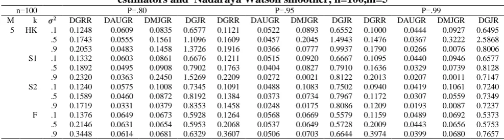
Table 6. MSE values of partially linear model using (DGRR), (DAUGRR), (DMJGRR)and(DGJR) estimators and Nadaraya Watson smoother, n=100,m=5

n=100 Ρ=.80 Ρ=.95 Ρ=.99

M k 𝝈𝟐 _{DGRR DAUGR DMJGR DGJR DGRR DAUGR DMJGR DGJR DGRR DAUGR DMJGR DGJR} 5 HK .1 0.1248 0.0609 0.0835 0.6577 0.1121 0.0522 0.0893 0.6552 0.1000 0.0444 0.0927 0.6495 .5 0.1743 0.0555 0.1561 1.1096 0.1609 0.0457 0.2045 1.4943 0.1476 0.0367 0.3222 2.5868 .9 0.2053 0.0483 0.1458 1.3726 0.1916 0.0366 0.0777 0.9937 0.1790 0.0266 0.0076 0.8006 S1 .1 0.1332 0.0603 0.0861 0.6676 0.1211 0.0515 0.0920 0.6667 0.1095 0.0440 0.0946 0.6577 .5 0.1892 0.0495 0.0908 0.7902 0.1763 0.0404 0.0827 0.7910 0.1636 0.0329 0.0739 0.8128 .9 0.2320 0.0363 0.2450 1.5269 0.2209 0.0272 0.0021 0.8122 0.2013 0.0207 0.0011 0.7147 S2 .1 0.1240 0.0575 0.1008 0.7345 0.1091 0.0488 0.1083 0.7502 0.0940 0.0419 0.1061 0.7240 .5 0.1589 0.0460 0.0872 0.8192 0.1384 0.0373 0.0734 0.7967 0.1172 0.0307 0.0559 0.7349 .9 0.1719 0.0331 0.0379 0.8353 0.1458 0.0248 0.0175 0.8086 0.1209 0.0193 0.0087 0.7237 F .1 0.1376 0.0649 0.0673 0.5928 0.1264 0.0568 0.0669 0.5579 0.1159 0.0489 0.0692 0.5373 .5 0.2146 0.0631 0.0654 0.5953 0.2068 0.0537 0.0649 0.5728 0.2009 0.0443 0.0656 0.5753 .9 0.3448 0.0614 0.0681 0.6329 0.3607 0.0506 0.0703 0.6644 0.3974 0.0399 0.0680 0.7657

3-From Table 7 when increasing the size of the sample to n= 400 and when 20.1 we find the partially linear model with proposed estimator (DGJR) that used third-order differences coefficients at most in the first place because it has less MSE. And partially linear model with proposed estimator(DMJGR ) alternated between

between second and third positions with the partially linear model with the estimator(DGRR). From Table 8 and 2 0.1 _{we find that the partially} linear model with proposed estimator(DMJGR) when using the fourth- order differences coefficients topped the first place followed by the partially linear model with the estimator (DAUGRR) then the estimator (DGJR)and then came the partially linear model with the estimator (DGRR) in the last position. When the variance increased to



2 0.5,0.9 we find that the partial linear model with the (DAUGRR) estimator in the first place and the partial linear model with (DMJGR) estimator alternates with the partially linear model with estimator (DGRR) on the second and third positions and the partially linear model

with proposed estimator(DGJR) was the last. The partially linear models with proposed estimators (DMJGR) and (DGJR) are in the first places when used the fifth-order differences coefficients and

1 . 0

2_

 _{as we observe from Table 9. When}

9 . 0 , 5 . 0

2

 then the partially linear model with estimator (DAUGRR) at most in the first place, and the partially linear models with the proposed estimators were at the last positions. By increasing the degree of correlation to 0.95,0.99 i.e. Increasing the degree of the multicollinearity we find that the partially linear model with proposed estimator (DMJGR) in second place at most, especially at the shrinkage parameters Ks1 and KHB and 20.5

Table 7. MSE values of partially linear model using (DGRR), (DAUGRR), (DMJGRR)and(DGJR) estimators and Nadaraya Watson smoother, n=400,m=3

n=400 Ρ=.80 Ρ=.95 Ρ=.99

M K 𝝈𝟐 DGRR DAUGR DMJGR DGJR DGRR DAUGR DMJGR DGJR DGRR DAUGR DMJGR DGJR

3 HK .1 0.0870 0.0411 0.0381 0.0111 0.0792 0.0364 0.0323 0.0290 0.0718 0.0534 0.0319 0.0251 .5 0.0880 0.0341 0.5268 3.8382 0.0782 0.0292 17.4648 136.1754 0.0689 0.0245 0.5560 5.6718 .9 0.0794 0.0290 0.5431 11.4032 0.0696 0.0239 1.0720 31.6807 0.0603 0.0193 2.5461 118.4718 S1 .1 0.0871 0.0407 0.0424 0.0086 0.0792 0.0360 0.0410 0.0085 0.0717 0.0313 0.0383 0.0028 .5 0.0980 0.0320 0.0762 0.0561 0.0952 0.0268 0.0510 0.0559 0.0927 0.0223 0.0318 0.1366 .9 0.1661 0.0253 0.0301 0.2469 0.1922 0.0159 0.0745 0.4327 0.2729 0.0183 1.5578 3.4699 S2 .1 0.0884 0.0401 0.0432 0.0012 0.0803 0.0353 0.0405 0.0022 0.0723 0.0308 0.0357 0.0121 .5 0.0803 0.0328 0.0458 0.0881 0.0680 0.0275 0.0398 0.1042 0.0558 0.0227 0.0399 0.1002 .9 0.0615 0.0264 0.0652 0.1002 0.0485 0.0220 0.0633 0.0928 0.0364 0.0183 0.0603 0.0879 F .1 0.0870 0.0399 0.0513 0.0223 0.0791 0.0360 0.0408 0.0219 0.0717 0.0321 0.0472 0.0174 .5 0.0810 0.0378 0.8732 2.7709 0.0783 0.0306 3.8519 8.9843 0.0736 0.0662 29.4580 1.8049 .9 0.0980 0.0963 694.8653 3.3471e+03 0.0916 0.0260 322.0688 2.4667e+03 0.0854 0.0277 282.3270 1.7594e+03

Table 8. MSE values of partially linear model using (DGRR), (DAUGRR), (DMJGRR)and(DGJR) estimators and Nadaraya Watson smoother, n=400,m=4

n=400 Ρ=.80 Ρ=.95 Ρ=.99

M k 𝝈𝟐 DGRR DAUGR DMJGR DGJR DGRR DAUGR DMJGR DGJR DGRR DAUGR DMJGR DGJR

4 HK

.1 0.1092 0.0466 0.0281 0.0782 0.0994 0.0414 0.0255 0.0782 0.0900 0.0362 0.0210 0.0868 .5 0.1132 0.0401 0.0791 0.7270 0.1012 0.0343 0.1999 1.3951 0.0896 0.0290 1.0190 6.3904 .9 0.1060 0.0341 0.3256 3.0530 0.0938 0.0288 0.1708 2.2274 0.0822 0.0239 0.2276 3.5786

S1

.1 0.1094 0.0462 0.0296 0.0704 0.0995 0.0409 0.0309 0.0555 0.0900 0.0357 0.0300 0.0499 .5 0.1480 0.0384 0.1837 0.5191 0.1208 0.0322 0.0638 0.0160 0.1209 0.0267 0.0446 0.0968 .9 0.2468 0.0311 0.0612 0.1375 0.3274 0.0259 0.0482 0.1832 0.7540 0.0214 0.0306 0.2263

S2

.1 0.1108 0.0455 0.0319 0.0689 0.1007 0.0400 0.0303 0.0650 0.0907 0.0349 0.0272 0.0660 .5 0.1054 0.0389 0.0399 0.1298 0.0908 0.0330 0.0336 0.1464 0.0763 0.0271 0.0328 0.1503 .9 0.0886 0.0327 0.0580 0.1507 0.0726 0.0269 0.0581 0.1463 0.0574 0.0220 0.0585 0.1387

F

Table 9. MSE values of partially linear model using (DGRR), (DAUGRR), (DMJGRR)and(DGJR) estimators and Nadaraya Watson smoother, n=400,m=5

n=400 Ρ=.85 Ρ=.90 Ρ=.99

M K 𝝈𝟐 DGRR DAUGR DMJGR DGJR DGRR DAUGR DMJGR DGJR DGRR DAUGR DMJGR DGJR

5 HK .1 0.1342 0.0590 0.0418 0.0569 0.1210 0.0594 0.0381 0.0524 0.1085 0.0728 0.0321 0.0460 .5 0.1343 0.0519 0.2464 1.7356 0.1217 0.0462 0.8923 5.9618 0.1091 0.0419 4.4816 37.3697 .9 0.1293 0.0417 502.8842 7.7395e+03 0.1131 0.0336 6.7534 89.5742 0.0967 0.0298 0.5696 8.1270 S1 .1 0.1360 0.0584 0.0435 0.0481 0.1229 0.0520 0.0438 0.0351 0.1105 0.0456 0.0417 0.0328 .5 0.1513 0.0494 0.1686 1.1583 0.1435 0.0419 0.0535 0.1082 0.1395 0.0349 0.0580 0.51642 .9 0.3096 0.0419 2.9885 17.9147 0.5080 0.035 0.0729 0.7244 2.9014 0.0299 0.0229 0.2817 S2 .1 0.1367 0.0579 0.0466 0.0464 0.1230 0.0510 0.0447 0.0421 0.1095 0.0447 0.0417 0.0405 .5 0.1142 0.0499 0.0646 0.0888 0.0950 0.0427 0.0574 0.1007 0.0762 0.0356 0.0504 0.1158 .9 0.0832 0.0424 0.0815 0.1227 0.0622 0.0356 0.0727 0.1371 0.0452 0.0301 0.0646 0.1470 F .1 0.1366 0.0568 0.0141 0.0171 0.1237 0.0514 0.0122 0.0157 0.1115 0.0460 0.0065 0.0141

.5 0.1226 0.0557 1.4165 5.0732 0.1158 0.0480 9.1252 25.7799 0.1072 0.0743 204.0168 159.9412

.9 0.1386 0.0565 42.5391 224.0120 0.1280 0.0522 29.8226 146.5994 0.1179 0.0477 31.8061 153.7311

Table 10. Shows the frequency of each method according to sample size

Sample size Methods

n=50 n=100 n=400

DGRR 57 20 -

DAUGRR 19 46 70

DMJGR 11 42 20

DGJR 21 - 18

Conclusion:

This study, proposes two estimators (DMJGR) and (DGJR) for partially linear models in which explanatory variables of parametric components suffer from the problem of multicollinearity. The performance of the partially linear models using proposed estimators (DMJGR) and (DGJR) are compared with that using the estimators (DGRR) and (DAUGRR) by means of the comparison criterion MSE. It is found that when the sample size is small, the partially linear models with proposed estimators (DMJGR) and (DGJR) are the best when using third –order differences coefficients. When the sample size is increased we find that the partially linear models with proposed estimator (DMJGR) are the best when using the fourth -order differences coefficients and when the variance is small. In some shrinkage parameters we see that the estimator (DMJGR) is the best when using a fifth –order differencing coefficients and when the degree of multicolinearity is very large and when the variance increased. When the size of the sample increased dramatically we find that the partially linear model with proposed estimate (DGJR) is the best at a third-order differences coefficients and when the variance is small. When order of differences coefficients increased we find that the partially linear models with proposed estimators at the first mattress especially at the differences coefficients of the fifth - order and when the variance is small. In general, we can observe the order of the methods according to sample sizes as shown in Table (10).

Conflicts of Interest: None.

References

1. Yatchew A. An elementary estimator of the partial linear model. Econ. Lett. 1997; 57: 135–143.

2. Wang L, Brown LD, Cai TT. A difference-based approach to semiparametric partial linear model. Department of Statistics, The Wharton School University of Pennsylvania, Pennsylvania, Technical report. 2007

3. Hoerl AE, Kennard R. Ridge regression: Biased estimation for non-orthogonal problems. TECHNOMETRICS. 1970a; 12:55-67.

4. Hoerl AE, Kennard R. Ridge regression: Application for non-orthogonal problems. TECHNOMETRICS. 1970b; 12:69-82.

5. Tabakan G, Akdeniz F. Difference-based ridge estimator of parameters in partial linear model. STAT PAP. 2010; 51(2):357–368

6. Duran EA, Akdeniz A. New difference-based estimator of parameters in semiparametric regression models. J STAT COMPUT SIM. 2011; 1-15 7. Duran EA, Härdle WK, Osipenko M.

Difference-based ridge and Liu type estimators in semiparametric regression models. J MULTIVARIATE ANAL. 2012; 105(1):164–175.

8. Roozbeh M, Arashi M, Kibria BM. Generalized ridge regression estimator in Semiparameteric regression models. JIRSS. 2015; 14(1):25-62

9. Akdeniz F, Duran EA, Roozbeh M, Arashi M. Efficiency of the Generalized Difference-based Liu Estimators in semiparametric Regression Models with Correlated Errors. J STAT COMPUT SIM. 2015; 85(1): 147-165.

10.Wu J. performance of the difference‑based almost unbiased Liu type estimator in partial linear model. J STAT COMPUT SIM. 2016

11.Wu J. Difference‑based ridge‑type estimator of parameters in restricted partial linear model with correlated errors. Wu Springer plus. 2016; 5:178 12.Wu J. A Jakknifed difference-based ridge estimator in

the partial linear model with correlated errors. A journal of theoretical and applied statistics. 2016; 50(6):1363-1375.

approach. international journal of soft computing. 2016; 11(5):295-298

14.Akdeniz F, Roozbeh M. Generalized Difference-based Weighted Mixed Almost Unbiased Ridge Estimator in Partially Linear Models. STAT PAP. 2017; 1–23.

15.Hussein SM, Hassan AH. Comparison of the suggested method (DBMJRR) with some estimators in the semi-parametric regression model using simulations. The 14th International Scientific Conference, Iraqi Statistical Association. 2017. 16.Wu J. Improvement of generalized difference-based

mixed Liu estimator in partially linear model. COMMUN STAT THEORY. 2018; 47(18): 4433-4442

17.Yatchew A. Semiparametric Regression for the Applied Econometrician. Cambridge, UK :Cambridge University Press; 2003.

18.Batah FS, Ramnathan TV, Gore SD. The Efficiency of Modified Jackknife and Ridge Type Regression Estimators: A comparison. Surveys in Mathematics and its Applications. . 2008;24(2):157-174.

19.Li Y, Yang H. On the performance of the jackknifed modified ridge estimator in the linear regression model with correlated or heteroscedastic errors. COMMUN STAT THEORY. 2011; 40:2695-2708. 20.Hassan AH. using difference technique in estimating

semiparametric regression model under semi complete multicollinearity problem with practical application. MS.c [thesis]. Baghdad:university of Baghdad; 2017.

21.Batah FS. A New Estimator by Generalized Modified Jackknife Ridge Regression Estimator. J.

of Basrah Researches ((Sciences)). 2011;37( 4) C:138-149.

22.Hussein SM, Yousif H. compared the proposed method (AUGJRR) with biased methods to estimate the Generalized ridge regression of the existence of multicollinearity. J. of Al-Rafidian University College for Sciences. 2016; 37: 69–99.

23.Yousif H. A comparisons among the Generalized Ridge regression methods of estimators under multicollinearity problem with a praxis. MS.c [thesis]. Baghdad: university of Baghdad; 2014. 24.Hussein SM, Hassan AH. Employing difference

technique in some liu estimators to semiparametric regression model. Diyala j. pure Sciences. 2017;13(4):24-37.

25.Akdeniz F, Erol H. Mean Squared Error Mattrix Comparisons of Some Biased Estimators in Linear Regression. COMMUN STAT THEORY. 2003; 32(12): 2389-2413.

26.Fan J, Gijbels I. Local Polynomial Modeling and Its Applications. CRC PRESS; 2003.

27.McDonald GC, Galarneau DI. A Monte Carlo evaluation of some Ridge-type estimators. J Amer Statist Assoc. 1975; 70:407–416.

28.Akdeniz F, Roozbeh M. Efficiency of the Generalized Difference-based Weighted Mixed Almost Unbiased two Parameter Estimator in Partially Linear Model. COMMUN STAT THEORY. 2017; 46(24): 12259-12280

29. Hussein SM. Alternative Estimators in Logit Model in The Presence of Multicollinearity and Heteroscedasticity with A stochastic Linear Restricted. IJAMAS. 2017;56 (4):169-181

ةنراقم

ضعب

لا

ردقم

تا

ةحرتقملا

ىلع

ساسأ

ةينقت

لا

قورف

يف

جذومنلا

يطخلا

يئزجلا

مادختساب

ةاكاحملا

نيسح دمحم ىجس

ءاصحلاا مسق ،

داصتقلااو ةرادلاا ةيلك ،

دادغب ةعماج .قارعلا ،دادغب ،

:ةصلاخلا

ممعملا لدعملا فيانكاجلا فرحلا رادحنا ردقم يهو قورفلا ةينقت ساسا ىلع ةينبم قئارط ميدقت مت ثحبلا اذه يف

ساسا ىلع

قورفلا ( DMJGR )

ردقمو ممعملا فيانكاجلا فرحلا رادحنا قورفلا ساسا ىلع

( DJGR ) يف ريدقت تاملعم ءزجلا يطخلا نم جذومنلا

يطخلا يئزجلا . امأ ةبسنلاب ءزجلل ريغ يطخلا لثمملا ةلادلاب ،ةيملعملالا دقف

مت هريدقت ردقم مادختساب Nadaraya Watson

تمت . ةنراقم

جذومنلا يطخلا يئزجلا مادختساب هذه قئارطلا ةحرتقملا عم تاردقم ىرخأ دمتعت ىلع ةينقت قورفلا نم للاخ رايعم ةنراقم MSE يف ةسارد

.ةاكاحم

:ةيحاتفملا تاملكلا ،قورفلا ةينقت

DGRR ، DAUGRR ،

DMJGR ،