Remote Sensing and GIS for Hydrology and Water Resources (IAHS Publ. 368, 2015) (Proceedings RSHS14 and ICGRHWE14, Guangzhou, China, August 2014).
33
Snow evolution in a semi-arid mountainous area combining
snow modelling and Landsat spectral mixture analysis
RAFAEL PIMENTEL
1, JAVIER HERRERO
2& MARÍA JOSÉ POLO
11 Fluvial Dynamics and Hydrology Research Group. Andalusian Institute for Earth System Research. University of Cordoba. Campus Rabanales, Edificio Leonardo da Vinci, Área de Ingeniería Hidráulica, 14017, Cordoba, Spain [email protected]
2 Fluvial Dynamics and Hydrology Research Group. Andalusian Institute for Earth System Research. University of Granada. Edificio CEAMA, Av del Mediterráneo s/n, 18006, Granada, Spain
Abstract This study proposes the use of both physically-distributed hydrological modelling in combination with satellite remote sensing images, to study the evolution of the snowpack in the Sierra Nevada mountains, in southern Spain. The snowmelt-accumulation module inside WiMMed (Watershed Integrated Management in Mediterranean Environment) hydrological model was employed, which includes the use of depletion curves to expand the energy and water balance equations over a grid representation. Snow maps obtained from spectral mixture analysis of Landsat images were used to evaluate this model at the study site. The results show a significant agreement between observed and simulated snow pixels in the area, which allows production of sequences of snow maps with greater resolution than the remote sensing images employed. However, some mismatches do appear at the boundaries of the snow area, mainly related to: (a) the great number of mixed pixels; and (b) the influence of the snow transport by wind.
Key words snow; physical modelling; spectral mixture analysis; semiarid environments; Landsat imagery; Spain
INTRODUCTION
Water from the melting of the snowpack is a basic resource for human consumption, agriculture irrigation or hydroelectric production in mountainous areas. Snow dynamics is conditioned on one hand by snow accumulation, redistribution and ablation, and the associated meteorological driving processes, and on the other hand by the influence of rough topography, with strong gradients of exposure, vegetation and shadowing. All these factors can be highly variable in Mediterranean environments, which increases the heterogeneity of snow distribution and makes it difficult to monitor and measure its evolution. Furthermore, spatially distributed hydrological modelling has become one of the most commonplace techniques for its study. Besides reproducing the physical processes involved in snow dynamics, models can produce a spatial distribution of snow at the scales significant for the reproduced processes, i.e. small catchment at high spatial resolution, or large catchment at very small resolution. A great effort has been dedicated to develop physical snow models, with different examples in the literature (Jordan, 1991; Tarboton et al., 1994; Marks
et al., 1999). In semi-arid regions, special considerations must be included (Herrero et al., 2009), such as highlighted from the analysis of a point snowmelt-accumulation model in Sierra Nevada (southern Spain). However, the extension of physical models to large areas in such regions requires the scaling-up from point to cell calculations; this is usually made through the use of depletion curves, which also captures subgrid variability (Luce et al., 1999), and the availability of distributed snow measurements, which is achieved by means of satellite-based snow observations, used in the calibration and validation steps (Schmugge et al., 2002). The snow variable most extensively employed in these processes is the snow cover fraction (SCF), due to the feasibility of obtaining it from remote sensing sources (Parajka and Blöschl, 2008). In semi-arid regions, the extremely changing conditions favour the particularly distributed pattern of the snow, which usually appears as medium to small sized patches. This is a limiting factor which is why Landsat imagery (30 × 30 m spatial resolution) is the most recommended for studying snow evolution over these areas (Marks and Winstral, 1999; Pimentel et al., 2012).
Obtaining snow maps from Landsat images is easy following the physical properties of the snow along the electromagnetic spectrum. The use of the Normalized Difference Snow Index (NDSI), which compares the visible and near infrared bands allows the discrimination between snow covered and non-covered pixels (Dozier, 1989; Herrero et al., 2011). However, when a
subgrid classification is required, a spectral mixture analysis can be applied (Painter et al., 2009). These techniques assume that the reflectance measured by the sensor from a given cell is a combination of the individual reflectances of the different kind of surfaces present within the endmembers.
This work analyses the spatial distribution regime of snow in the Sierra Nevada mountains (Spain) at the subgrid scale by means of application of the point snowmelt-accumulation model developed by Herrero el al. (2009), and obtaining a 10-year series of snow cover fraction maps from a spectral mixture model applied to Landsat imagery.
STUDY SITE AND AVAILABLE DATA
This study site was in the Sierra Nevada Mountains, southern Spain. They are a linear mountain range parallel to the coastline of the Mediterranean Sea, with altitudes from 1500 to 3500 m a.s.l. The typical mountain alpine climate is modified by its proximity to the sea, which generates semi-arid and tropical conditions in the surrounding area, mainly on the southern hillside closer to the sea. The study area selected was the Guadalfeo River basin upstream of Rules Dam, with an extent of 1057.3 km2, which has been previously studied and hydrologically modelled.
Fig. 1 Location of Sierra Nevada Mountain Range in Spain, limits of the study area (black line), Rules Dam (white cross) and weather stations employed in the study (black crosses).
Different weather station networks are available in this area; in this work, hourly and daily datasets of precipitation, temperature, radiation (shortwave and longwave), pressure, wind velocity, and relative humidity from the Agroclimatic Information Network of Andalusia (RIA) and the Guadalfeo Project Network (Herrero et al., 2011) were employed as input to the snow model. Specific interpolation algorithms were used in this abrupt topography, including, in the case of temperature and precipitation, the consideration of residual conditioned by the altitudinal gradients (Herrero et al., 2007) and, for radiation, topographic effects are also considered (Aguilar
et al., 2010).
METHODS
The accumulation–snowmelt cycles during the ten years from 2004 to 2013 were simulated at the study site using the physical and distributed model developed and calibrated by Herrero et al.
Snow model
The snowmelt-accumulation model for Mediterranean sites developed by Herrero et al. (2009) is a physical model based on a point mass and energy balance, which is extended to a distributed way by means of depletion curves (Herrero et al., 2011).
The model assumes a uniform horizontal snow cover surface distributed in one vertical layer. In the control volume defined by the snow column per unit area, which has the atmosphere as an upper boundary and the ground as a lower one, the water mass and energy balance can be expressed by equations (1) and (2):
𝑑𝑑𝑑𝑑𝑑𝑑𝑑𝑑
𝑑𝑑𝑑𝑑 = 𝑅𝑅 − 𝐸𝐸 + 𝑊𝑊 − 𝑀𝑀 (1)
𝑑𝑑(𝑑𝑑𝑑𝑑𝑑𝑑·𝑢𝑢)
𝑑𝑑𝑑𝑑 =
𝑑𝑑𝑑𝑑
𝑑𝑑𝑑𝑑 = 𝐾𝐾 + 𝐿𝐿 + 𝐻𝐻 + 𝐺𝐺 + 𝑅𝑅 · 𝑢𝑢𝑅𝑅− 𝐸𝐸 · 𝑢𝑢𝑑𝑑+ 𝑊𝑊 · 𝑢𝑢𝑑𝑑− 𝑀𝑀 · 𝑢𝑢𝑀𝑀 (2) where SWE (snow water equivalent)is the water mass in the snow column, and u is the internal energy per unit of mass (U for total internal energy). In the mass balance, R defines the precipitation rate; E is water vapour diffusion rate (evaporation/condensation); W represents the mass transport rate due to wind; and M is the melting water rate. Regarding energy fluxes, K is the solar or short wave radiation; L the thermal or long-wave radiation; H the exchange of sensible heat with the atmosphere rate; G the heat exchange with the soil rate; and uR, uE, uW and uMare the
advective heat rate terms associated with each of the mass fluxes involved in equation (1).
This approach permits an easy extension to a distributed model by means of making calculations simultaneously in each cell. However, a direct extension cannot be done when the cell area is not completely covered by snow. In such cases, the parameterization of subgrid processes is made by including depletion curves, which are empirical functions that relate the fraction of cell area covered by snow with some other snow state variables, and quantify the decrease in snow cover within the cell to take into account the reducing of the area implied in the energy-mass balance.
Landsat imagery
This section describes firstly the different levels of pre-processing needed to transform row image digital numbers into reflectance values, and secondly the method employed to obtain snow cover maps from these datasets.
Preprocessing is composed of four different, sequential steps: radiometric, atmospheric, saturation and topographic corrections. First, radiometric calibration by means of rescaling factors (Chander et al., 2009) to transform calibrated Digital Number in the original images into radiance values at the sensor was applied. Secondly, the atmospheric Dark Object Subtraction (DOS), was selected; this algorithm assumes that all atmospheric effects are represented by a blackbody in the image, which by definition must absorb all the solar radiation (Chavez, 1996), and together with this assumption, several simplifications on the reflectance physics equation, such as a Lambertian surface and a cloudless atmosphere, are done. After the atmospheric correction, the reflectance values obtained require additional corrections due to the saturation problems that usually appear in these snow areas associated with the radiometric configuration of the satellite. Based on the hypothesis of a high correlation between spectral bands for snow, a multivariate correlation analysis between bands was made to recover the snow saturated pixels values (Karnieli et al., 2004). Finally, a C-correction with the land cover separation algorithm (Hantson and Chuvieco, 2011) was employed to homogenize direct solar and non-solar illuminated areas in this rough mountainous terrain.
𝑁𝑁𝑁𝑁𝑁𝑁𝑁𝑁 = (𝑇𝑇𝑀𝑀2 − 𝑇𝑇𝑀𝑀5) (𝑇𝑇𝑀𝑀2 + 𝑇𝑇𝑀𝑀5)⁄ (3) where TMi correspond to the reflectance value in Landsat band i. On the other hand, linear spectral mixture analysis was employed to estimate the snow cover fraction within each pixel in all the images (Painter et al., 2009). This analysis assumes that the reflectance measured at the sensor,
R
S,λ, is a linear combination of the reflectance values from each spectral endmember, that is, puresurface covers present in the area:
𝑅𝑅𝑑𝑑,𝜆𝜆= ∑𝑁𝑁𝑖𝑖=1𝐹𝐹𝑖𝑖𝑅𝑅𝜆𝜆,𝑖𝑖+ 𝜀𝜀𝜆𝜆 (4)
where
F
i is the fraction of the endmember i;R
λ,i is the reflectance obtained after the distinctpre-processing steps of endmember i at wavelength
λ
; N is the number of spectral endmembers taken into account; andε
λ is the residual error atλ
associated with the fit of the N endmembers. Theleast-squares fit to
F
i is solved by means of a reflective Newton method.Three significant endmembers were identified in the study area, snow, vegetation (brush creeping vegetation) and rocks (phillite), their spectrum being obtained from a digital spectral library (http://speclab.cr.usgs.gov/).
RESULTS AND DISCUSSION Snow cover fraction maps
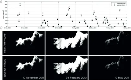
Snow maps during the 10-year series of Landsat images were obtained from both methodologies. Figure 2(a) shows the evolution of the global snow area at the study site throughout the period 2004–2013. Parallel temporal trends can be observed, with overestimated values of SCF when binary maps are employed, as expected, since there is a threshold over which this analysis results in a covered classification. This is particularly relevant during accumulation phases, with maximum differences usually obtained for the peak SCF values over a complete cycle. Melting stages generally exhibit closer values, especially during the final melting cycle of each hydrological year.
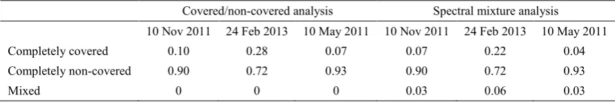
A root mean squared error (RMSE) of 15.6 km2 was obtained by comparing both kinds of results over the study period, which represents a notable improvement with using the spectral mixture analysis given that the maximum snow cover area found ranged from 370 to 130 km2. The snow distribution is shown in Fig. 2(b) for three selected dates during the study period, associated with different states throughout the snow season (beginning of accumulation, consolidated snow and beginning of melting). Moreover, Table 1 includes the fraction of area associated with cover (SCF = 1), non-covered (SCF = 0) and mixed (0 < SCF < 1) situations for these dates at the study site, for both classification algorithms.
Obviously, the covered/non-covered analysis does not discriminate mixed cells. The results show that the non-covered area is adequately represented by this algorithm; however, a significant portion of cells considered as snow-covered do not correspond to SCF = 1, with an associated area that can be close to a 40% of the estimated snow area by the covered/non-covered analysis. These mismatched pixels are usually located within border sites, as can be seen in Fig. 2(b), where the interaction between the melting snow and rocks is stronger.
Table 1 Fraction values of each type of area considered in the analysis (completely covered, completely non-covered and mixed) obtained from both algorithms for the 10 Nov 2011, 24 Feb 2013 and 10 May 2011 Landsat TM images.
Covered/non-covered analysis Spectral mixture analysis
10 Nov 2011 24 Feb 2013 10 May 2011 10 Nov 2011 24 Feb 2013 10 May 2011
Completely covered 0.10 0.28 0.07 0.07 0.22 0.04
Completely non-covered 0.90 0.72 0.93 0.90 0.72 0.93
Mixed 0 0 0 0.03 0.06 0.03
Snow cover simulations
The 10-year study period was simulated by the distributed snow model previously described, with the calibration values obtained by Herrero et al. (2009). Figure 3 shows the comparison of the average SCF value in the watershed simulated over the study period and the average SCF value obtained from each Landsat image. A good level of accuracy of the simulation can be generally observed. A global RMSE of 0.05 m2 m-2, associated with 50 km2 of snow area values, was found.
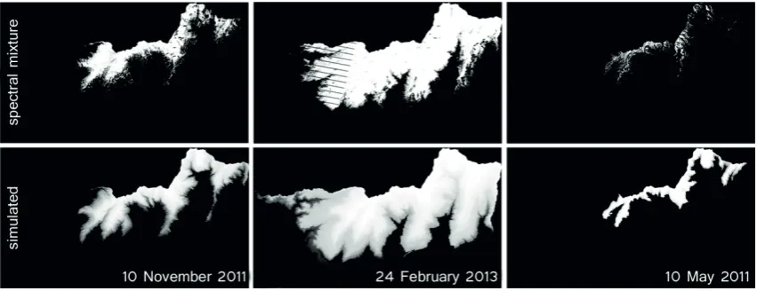
Figure 4 shows a comparison between the spatial simulated and observed distribution of snow throughout the watershed for the three selected images, including snow maps. As can be observed, again the border cells are not always correctly represented. Moreover, some snow free areas do appear inside the completely covered area that are not represented by the model; this characteristic snow distribution can be usually found and is generally due to wind effects. The model does not consider redistribution of snow by wind transport and therefore these mismatches are likely to appear when windy conditions between two consecutive images are not negligible.
CONCLUSIONS
The distribution of snow cover under highly variable conditions was estimated by spectral mixture analysis of Landsat images, which has proved to be a powerful tool for providing time map series to be used in snow modelling. The spectral mixture analysis allows an adequate estimation of the coverage of snow in each pixel of the area, which resulted in a global reduction of the snow cover area of close to 40% in the mixed identified cells when compared to a simple covered/non-covered classification analysis, this being especially important in these semi-arid mountainous regions where the particular snow dynamics favour the appearance of a great number of mixed pixels.
Fig. 3 Evolution of mean SCF over the watershed. Black line represents simulated values and black dots are the estimates from spectral mixture analysis of Landsat imagery.
Fig. 4 Comparison between measured (up) and simulated (down) snow cover fraction maps for selected dates 10 November 2011 (RMSE = 0.261 m2 m-2); 24 February 2013 (RMSE = 0.180 m2 m-2) and 10 May 2011 (RMSE = 0.301 m2 m-2).
Acknowledgements This work was partially funded by the Spanish Ministry of Science and Innovation (Research Project CGL 2011-25632, “Snow dynamics in Mediterranean regions and its modelling at different scales. Implications for water management”), and the Biodiversity Foundation, Spanish Ministry of Agriculture, Food and Environment (Project “Study of the effect of global change on snow and high mountain hydrology in Sierra Nevada National Park”). Moreover the present work was partially developed within the framework of the Panta Rhei Research Initiative of the International Association of Hydrological Sciences (IAHS) (Working Groups Water and energy fluxes in a changing environment and Mountain Hydrology).
REFERENCES
Aguilar, C., Herrero, J. and Polo, M.J. (2010) Topographic effects on solar radiation distribution in mountainous watersheds and their influence on reference evapotranspiration estimates at watershed scale. Hydrol. Earth Syst. Sci. 14(12), 2479–2494. Chander, G., Markham, B. L. and Helder, D. L (2009) Summary of current radiometric calibration coefficients for Landsat
MSS, TM, ETM+, and EO-1 ALI sensors. Remote Sens. Environ. 113(5), 893–903.
Chavez, P. (1996) Image-based atmospheric corrections-revisited and improved. Photogramm. Eng. Remote Sens. 62(9), 1025–1036. Hantson, S. and Chuvieco, E. (2011) Evaluation of different topographic correction methods for Landsat imagery. Int. J. Appl.
Earth Obs. Geoinf. 13(5), 691–700.
Herrero, J., et al. (2007) Mapping of meteorological variables for runoff generation forecast in distributed hydrological modelling. Proc. Hydraulic Measurements & Experimental Methods, 606–611.
Herrero, J., Polo, M. J. and Losada, M. A. (2011) Snow evolution in Sierra Nevada (Spain) from an energy balance model validated with Landsat TM data. Proc.Remote Sensing for Agriculture, Ecosystems and Hydrology, 8174, 817403. Herrero, J., et al. (2009) An energy balance snowmelt model in a Mediterranean site. J. Hydrol, 371(1-4), 98–107. Jordan, R. E. (1991) A one-dimensional temperature model for a snow cover, CRREL Special Reports.
Karnieli, A., et al. (2004) Radiometric saturation of Landsat-7 ETM+ data over the Negev Desert (Israel): problems and solutions. Int. J. Appl. Earth Obs. Geoinf. 5(3), 219–237.
Luce, C., Tarboton, D. and Cooley, K. (1999) Subgrid parameterization of snow distribution for an energy and mass balance snow cover model, Hydrol. Process.13, 1921–1933.
Marks, D., et al. (1999) A spatially distributed energy balance snowmelt model for application in mountain basins. Hydrol.
Processes 1935–1959.
Painter, T. H., et al. (2009) Retrieval of subpixel snow covered area, grain size, and albedo from MODIS. Remote Sens.
Parajka, J. and Blöschl, G. (2008) The value of MODIS snow cover data in validating and calibrating conceptual hydrologic models, J. Hydrol. 358(3-4), 240–258.
Pimentel, R., Herrero, J. and Polo, M. J. (2012) Terrestrial photography as an alternative to satellite images to study snow cover evolution at hillslope scale. Proc. Remote Sensing for Agriculture, Ecosystems and Hydrology, 8531.
Schmugge, T.J., et al. (2002) Remote sensing in hydrology. Adv. Water Resour. 25(8-12), 1367–1385.
Tarboton, D.G., Chowdhury, T.G. and Jackson, T.H. (1994) A spatially distributed energy balance snowmelt model. Reports