International Journal of Analysis and Applications Volume 17, Number 2 (2019), 191-207
URL:https://doi.org/10.28924/2291-8639 DOI:10.28924/2291-8639-17-2019-191
SOLUTIONS OF FRACTIONAL DIFFUSION EQUATIONS AND CATTANEO-HRISTOV DIFFUSION MODEL
NDOLANE SENE∗
1Laboratoire Lmdan, D´epartement de Math´ematiques de la D´ecision, Universit´e Cheikh Anta Diop de
Dakar, Facult´e des Sciences Economiques et Gestion, BP 5683 Dakar Fann, Senegal
∗Corresponding author: [email protected], [email protected]
Abstract. The analytical solutions of the fractional diffusion equations in one and two-dimensional spaces have been proposed. The analytical solution of the Cattaneo-Hristov diffusion model with the particular boundary conditions has been suggested. In general, the numerical methods have been used to solve the fractional diffusion equations and the Cattaneo-Hristov diffusion model. The Laplace and the Fourier sine transforms have been used to get the analytical solutions. The analytical solutions of the classical diffusion equations and the Cattaneo-Hristov diffusion model obtained when the order of the fractional derivative converges to 1 have been recalled. The graphical representations of the analytical solutions of the fractional diffusion equations and the Cattaneo-Hristov diffusion model have been provided.
1. Introduction
In fractional calculus, we have many fractional derivatives operators as: the Riemann-Liouville fractional
derivative [34] [36], the Caputo fractional derivative [8] [41], the Atangana-Baleanu fractional derivative
[2] [3] [4], the Caputo-Fabrizio fractional derivative [6] [30], the Conformable fractional derivative [42], the
generalized fractional derivatives in Caputo and Riemann-Liouville sense [21] [22] [24], and others. Fractional
calculus has many applications in mechanic, physics and science and engineering. Fractional calculus has
many applications in the viscoelastic models and the diffusion models. In [12] [13], Hristov treats on heat
Received 2018-12-03; accepted 2019-01-09; published 2019-03-01. 2010Mathematics Subject Classification. 42A38, 76R50, 26A33 .
Key words and phrases. Fractional diffusion equation; Caputo fractional derivative; Cattaneo-Hristov diffusion model.
c
2019 Authors retain the copyrights
of their papers, and all open access articles are distributed under the terms of the Creative Commons Attribution License.
diffusion equation in term of the Caputo-Fabrizio time fractional derivative. In [10], Hristov proposes new
equations related to the fractional diffusion equations using the Atangana-Baleanu fractional derivative, see
others models in [23]. In [1], Alkahtani and Atangana discuss the numerical solution of the Cattaneo-Hristov
diffusion equation. In [26] Koca et al. propose the numerical solution of the second term of the
Cattaneo-Hristov diffusion equation. In [27], Li et al. have studied the Cauchy problem for nonlinear fractional
time-space generalized Keller-Segel equation using the Caputo fractional derivative. In [29], Yranli et al.
devoted to comparing the smoothing performance between the time fractional diffusion equation and the
classical diffusion equation using the regulation method, Savitzky-Golay, and coverer method. In [37], Ruan
et al. study a simultaneous identification problem of piecewise source term and the fractional order for
time-fractional diffusion equation. In [45], Zhang and al. propose a discrete form for solving time fractional
convection-diffusion equation. In [31], Ma et al. study asymptotic of the solutions to the fractional anomalous
diffusion equations. Several works related to the fractional diffusion equations exist in the literature. The
papers [5] [33] [39] [44] treat on fractional diffusion equations.
The fractional diffusion equation is obtained when a specific fractional derivative operator replaces the
ordinary derivative in the classical diffusion equation. In this paper, we use the Caputo fractional
deriva-tive. Podlubny [35] has introduced the fractional diffusion equation in fractional calculus. We propose the
analytical solutions of the fractional diffusion equations in one and two-dimensional spaces. Hristov [12]
introduced the Cattaneo-Hristov diffusion equation in fractional calculus. The author [12] opens news
prob-lems related to the analytical or approximate solutions of the Cattaneo-Hristov diffusion equation. Koca
et al. [26] propose the numerical and analytical solutions of the elastic part of the heat diffusion equation
process. Alkahtani et al. [1] propose the numerical solution of the complete Cattaneo-Hristov diffusion
equa-tion using the Crank-Nicholson numerical scheme. Hristov [12] proposes an approximate solution of the
Cattaneo-Hristov diffusion equation using the heat-balance integral method (HBIM). Hristov [12] proposes
a double integral-balance method (DIM) to get the approximate solution of the Cattaneo-Hristov diffusion
equation. The analytical or approximate solutions of the fractional diffusion equations using HBIM and
DIM were proposed in [14] [15] [16] [17] [18] [19] [20] [32]. The analytical solution of the Cattaneo-Hristov
equation was stated in [26] by Koca et al. They give the analytical solution of the elastic part of the heat
diffusion equation process. In this paper, we continue the work concerning the analytical solution stated
by Koca et al. in [26]. In this paper, we propose the analytical solution of the complete Cattaneo-Hristov
diffusion equation of the transient heat equation using an integral method. The integral method uses both
the Fourier sine transform and the Laplace transform. We will notice this integration method will permit
to express the analytical solutions of the fractional diffusion equations in the term of the Gaussian error
function and the Mittag-Leffler function [9] [40]. The graphical representations of the analytical solutions of
Int. J. Anal. Appl. 17 (2) (2019) 193
The paper is organized as follows: in Section 2, we recall preliminary definitions which we will use in this
paper. In Section 3, we analyze the analytical solutions of the fractional diffusion equation in one-dimensional
space. In Section 4, we get the analytical solution of the fractional diffusion equation in two-dimensional
space. In Section 5, we analyze some particular cases graphically. And we finish with Section 6 by giving
the conclusions and remarks.
2. Fractional diffusion equations
In this section, we present the fractional differential equations studied in this paper. The problems concern
the fractional diffusion equation in one and two-dimensional spaces. The classical diffusion equation defined
by the ordinary derivative is popular. Many works related to the analytical and the numerical solutions
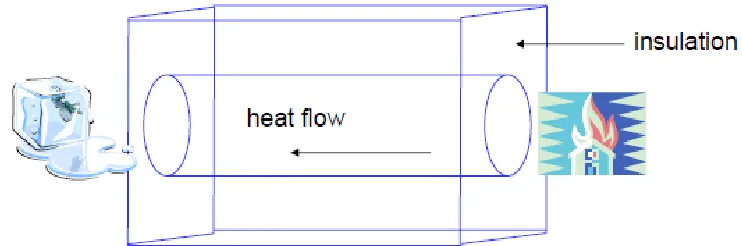
exist. Diffusion phenomena, of heat or mass [12] [35] is represented as the following form
∂u(x, t) ∂t =κ
2∂2u(x, t)
∂x2 (2.1)
whereκ2= K
ρCp. We add the following informations.
• • •K represents the thermal conductivity,
• • •ρrepresents the specific heat,
• • •Cprepresents the density of the material,
• • •urepresents the temperature distribution of the material.
The fractional diffusion equation is obtained when we replace the ordinary derivative by a fractional
derivative operators. The fractional diffusion equation described by the Caputo fractional derivative is
expressed in one-dimensional space by the following equation [11] [31] [35]
Dcαu(x, t) =κ2∂
2u(x, t)
∂x2 (2.2)
whereDc
αrepresents the Caputo fractional derivative operator defined by [28] [40]
Dαcu(x, t) = 1 Γ(1−α)
Z t
0
u0(x, s)
(t−s)αds (2.3)
all t > 0, α ∈ (0,1), and Γ(.) denotes the Gamma function. κ2 represents the diffusion coefficient for
the density of the diffusion material. The boundary conditions considered in this paper are the Dirichlet
boundary conditions:
• • •u(x,0) = 0 forx >0,
• • •u(0, t) = 1 fort >0.
The fractional diffusion equation exists in two dimensional space. It is expressed as the following form [31]
Dcαu(x, y, t) =κ2
∂2u(x, y, t)
∂x2 +
∂2u(x, y, t)
∂y2
(2.4)
• • •u(x, y,0) = 0 forx, y >0,
• • •u(0, y, t) =u(x,0, t) = 1 fort >0.
The initial boundary conditions play an important role in the integral method. Note that, when the
boundary conditions change, the form of the analytical solutions changes also. There exist many methods
to get the analytical solutions of the fractional diffusion equations: as the Laplace transform, as the Fourier
sine transform [43], as the heat-balance integral method (HBIM) [18,20], as a double integral method
(DIM) [18,20], as a multiple integral method (MIM) [14]. This paper proposes an integral method consisting
of applying both the Laplace transform and the Fourier sine transform. Let recall the Laplace transform of
the Caputo fractional derivative which we will use later [25] [38]
L {Dcαf(t)}=s α
L {f(t)}(s)−sα−1f(0) (2.5)
whereα∈(0,1). The transformation (2.5) is known very useful in the resolution of the fractional differential
equations. All solutions obtained in this paper will be rewritten using the Mittag-Leffler function [9] defined
as the following form
Eα,β(z) =
∞ X
k=0
zk
Γ(αk+β). (2.6)
where α >0, β ∈R andz ∈C. We obtain the exponential function when α=β = 1 and we obtain the
Mittag-Leffler function with one parameter whenβ= 1, for more information see in [9].
3. Analytical Solution of Fractional Diffusion Equation in One Dimensional space
In this section, we investigate to find the analytical solution of the fractional diffusion equation in
one-dimensional space defined as the following form
Dcαu(x, t) =κ2∂
2u(x, t)
∂x2 . (3.1)
We consider the Dirichlet boundary conditions defined as follows:
• • •u(x,0) = 0 forx >0,
• • •u(0, t) = 1 fort >0.
In other words, we assume that the initial temperature of the material is null and the temperature of the
plate for all t > 0 is maintained constant U0 = 1. It is essential for our results and the application of
our method of resolution. The integral methods as HBIM and DIM use the finite penetration depth to get
the approximate solutions of the fractional diffusion equation (3.1). For more information on these integral
methods, see in [18] [20]. In this paper, we adopt the following integral method (see in [43]), described as
follows:
• • •apply the Fourier sine transform,
Int. J. Anal. Appl. 17 (2) (2019) 195
Figure 1. Fractional diffusion model.
• • •apply the inverse of Laplace transform,
• • •apply the inverse of Fourier sine transform.
This method of resolution seems very useful and practical to get the analytical solution of the fractional
diffusion equations. If the temperature of the plate is null, the integral method described above seems no
adequate to be applied and it is better to use the classical methods as HBIM or DIM to solve equation (3.1).
We begin the resolution of the fractional differential equation (3.1) by applying the Fourier sine transform.
Multiplying equation (3.1) by 2πsinwxand integrating it between 0 to∞, we get that:
Dαcus(w, t) = κ2
2
πwus(0, t)−w
2u s(w, t)
Dαcus(w, t) =
2κ2w
π −κ
2w2u s(w, t).
whereus(w, t) denotes the Fourier sine transform ofu(x, t). Rearranging, we obtain the following fractional
differential equation defined as
Dcαus(w, t) +κ2w2us(w, t) =
2κ2w
π . (3.2)
The second step of the resolution consists of applying the Laplace transform to both sides of equation (3.2),
and then we obtain that
sαu¯s(w, s) +κ2w2u¯s(w, s) =
2κ2w
πs
¯
us(w, s) =
2κ2w
πs(sα+κ2w2). (3.3)
where ¯us(w, s) denotes the Laplace transform ofus(w, t). The third step of the resolution consists of applying
the inverse of the Laplace transform to both sides of equation (3.3). To reach our end, we rewrite equation
(3.3) as follows:
¯
us(w, s) =
2 π
1
s−
sα−1 sα+κ2w2
1
Applying the inverse of Laplace transform to both sides of equation (3.4) and using the Mittag-Leffler
function as defined in [9], we get
us(w, t) =
2 πw
1−Eα −κ2w2tα . (3.5)
To get the analytical solution of the fractional diffusion equation (3.1), we apply the inverse of the Fourier
sine transform to both sides of equation (3.5), and then we obtain the following result
u(x, t) = 2 π Z ∞ 0 sinwx w
1−Eα −κ2w2tα dw
= 1−2
π Z ∞
0
sinwx
w Eα −κ
2w2tα
dw. (3.6)
Let now analyze a particular case of the fractional diffusion equation. The classical diffusion equation is
obtained when α→ 1. To get the analytical solution, we use the Laplace transform obtained in equation
(3.3). We have the following decomposition
¯
us(w, s) =
2 π 1 s− 1 s+κ2w2
1
w. (3.7)
Using the inverse of Laplace transform to both sides of equation (3.7), we get the following intermediary
solution
us(w, t) =
2 πw
1−exp −κ2w2t . (3.8)
Respecting the procedure of the resolution, we have to apply the inverse of Fourier sine transform, and then
we obtain the analytical solution of the classical diffusion equation given by
u(x, t) = 2 π Z ∞ 0 sinwx w
1−exp −κ2w2t dw
= 1− 2
π Z ∞
0
sinwx
w exp −κ
2w2t dw
= 1−erf
x 2κ√t
(3.9)
where the functionerf(.) denotes the Gaussian error function.
Let’s give the behavior of the temperature distribution of the material in some configurations. See in figures
2,3,4 and 5 the behavior of the temperature distribution of the material u in different cases. The figure 2
describes the behavior of the temperature distribution of the material in the diffusion equation (α → 1)
when x and t take different values with the diffusion coefficient for the density of the diffusion material
fixed toκ2= 0.85.10−4m2/s(Hydrogen ion diffusion coefficient). The figure3describes the behavior of the
temperature distribution of the material in the diffusion equation (α→1) whenxtakes different values and
t→ ∞and with the diffusion coefficient for the density of the diffusion material fixed toκ2= 0.85.10−4m2/s.
We can observe all the curves decay rapidly. Thus the diffusion becomes more than more rapid. The figure4
Int. J. Anal. Appl. 17 (2) (2019) 197
Figure 2. Surface of the temperature distribution forα→1,κ2= 0.85.10−4m2/s
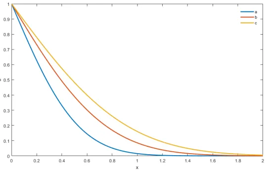
Figure 3. The temperatures distributions forα→1,κ2= 0.85.10−4m2/sandt→ ∞
successivelyx= 0.0050,x= 0.0065 andx= 0.0095 andt takes various values with the diffusion coefficient
for the density of the diffusion material fixed to κ2 = 0.85.10−4m2/s. We observe when x → 0 then the
temperature distribution of the material in the diffusion equation (α → 1) converge to 1. Furthermore,
we can observe all the curves increase slowly. Thus the diffusion is in general very slow. The figure 5
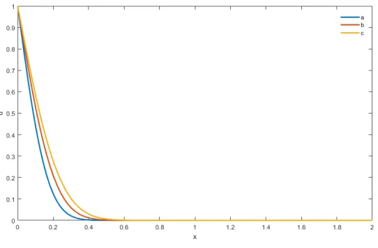
describes the behavior of the temperature distribution of the material in the diffusion equation (α → 1)
when successively t= 100,t= 150 andt= 200 andxtakes various values with the diffusion coefficient for
the density of the diffusion material fixed toκ2= 0.85.10−4m2/s. We can observe all the curves decay very
Figure 4. The temperatures distributions forα→1,κ2= 0.85.10−4m2/s, x= 0.0050; 0.0065; 0.0095
Figure 5. The temperatures distributions forα→1,κ2= 0.85.10−4m2/s,t= 100; 150; 200
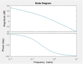
We use a bode plot to interpret the result of this paper graphically. To this end, we use the transfer
function given here by the Laplace transform. To reach our conclusion, we compute the capacity
H(s) = 2κ
2
πs(s+κ2w2)
using Matlab code, we obtain the behavior of the amplitude and the phase of the temperature distribution,
Int. J. Anal. Appl. 17 (2) (2019) 199
Figure 6. Bode plot of temperature distribution withα→1,κ= 0.85.10−4m2/s
4. Analytical Solution of the Fractional Diffusion Equation in Two Dimensional Space
In this section, we investigate to find the analytical solution of the fractional diffusion equation in
two-dimensional space expressed as follows
Dcαu(x, y, t) =κ 2
∂2u(x, y, t)
∂x2 +
∂2u(x, y, t)
∂y2
(4.1)
with Dirichlet boundary conditions defined as
• • •u(x, y,0) = 0 forx, y >0,
• • •u(0, y, t) =u(x,0, t) = 1 fort >0.
We repeat the same reasoning as in Section 3. We apply the Fourier sine transform. Multiplying equation
(4.1) by π2sinwxsinηyand integrating it between 0 to ∞successively respectingxandy, we get that:
Dαcus(w, η, t) = κ2
2(w2+η2)
πwη us(0, t)−(w
2+η2)u
s(w, η, t)
Dαcus(w, η, t) =
2κ2(w2+η2) πwη −κ
2(w2+η2)u
s(w, η, t).
where us(w, η, t) denotes the Fourier sine transform of u(x, y, t). Rearranging, we obtain the following
fractional differential equation defined as
Dαcus(w, η, t) +κ2(w2+η2)us(w, η, t) =
2κ2(w2+η2)
We apply the Laplace transform to both sides of equation (4.2). We obtain the following relationships
sαu¯s(w, η, s) +κ2(w2+η2)¯us(w, η, t) =
2κ2(w2+η2) πwηs
¯
us(w, η, s) =
2κ2(w2+η2)
πwηs(sα+κ2(w2+η2)). (4.3)
where ¯us(w, η, s) denotes the Laplace transform of us(w, η, t). To obtain the analytical solution of the
fractional diffusion equation (4.1), we rewrite the Laplace transform (4.3) as follows
¯
us(w, η, s) =
2 πwη
1 s−
sα−1 sα+κ2(w2+η2)
. (4.4)
Finally, to get the analytical solution of the fractional diffusion equation (4.1), we apply the inverse of Laplace
transform to both sides of equation (4.4) and the inverse of Fourier sine transform on the obtained equation.
We get
u(x, y, t) = 4 π2 Z ∞ 0 sinwx w Z ∞ 0 sinηy y
1−Eα −κ2(w2+η2)tα dηdw.
We investigate the analytical solution of the diffusion equation in two-dimensional space obtained when
α→1. To this end, we pick the Laplace transform function defined to equation (4.4) whenα→1, defined
by
¯
us(w, η, s) =
2 πwη
1
s−
1 s+κ2(w2+η2)
. (4.5)
Applying the inverse of Laplace transform and the inverse of the Fourier sine transform, we obtain that
u(x, y, t) = 4 π2 Z ∞ 0 sinwx w Z ∞ 0 sinηy y
1−exp −κ2(w2+η2)t dηdw
= 1− 4
π2 Z ∞ 0 sinwx w Z ∞ 0 sinηy
y exp −κ
2(w2+η2)t dηdw.
We use the Gaussian error functionerf(.), we obtain the following form
u(x, y, t) = 1−erf x
2κ√t
erf y
2κ√t
. (4.6)
That is the analytical solution of the diffusion equation in two-dimensional space obtained whenα→1.
Let’s give the behavior of the temperature distribution of the material in the diffusion equation in some
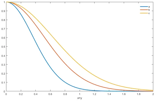
configurations. Figure7describes the behavior of the temperature distribution of the material in the diffusion
equation in two-dimensional space whenx=yandttakes various values. Figure8describes the behavior of
the temperature distribution of the material in the diffusion equation in two-dimensional space whenx=y
andt→ ∞, we observe the Gaussian profile of the temperature distribution of the material in the diffusion
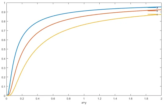
equation. Figure 9 describes the behavior of the temperature distribution of the material in the diffusion
equation in two-dimensional space whenx=y→0 andttake various values. We observe all curves increase
Int. J. Anal. Appl. 17 (2) (2019) 201
Figure 7. Surface of the temperature distribution of the material in the diffusion equation
forα→1,κ= 0.85.10−4m2/s,x=y
Figure 8. Temperature distribution of the material in the diffusion equation for α→ 1,
κ= 0.85.10−4m2/s,x=y andt→ ∞
5. Analytical Solution of the Cattaneo-Hristov Diffusion Equation
Hristov in [12] [13], stating with Cattaneo constructive relaxation with Jeffrey’s kernel proposes a new
elastic heat diffusion equation described by the Caputo-Fabrizio fractional derivative. Diffusion phenomena,
of heat or mass, are generally explained as a consequence of the conservative law by the relationships [12]
ρCp
∂T ∂t =−
∂q
∂x; q(x, t) =−k
∂T(x, t) ∂x ⇒ρCp
∂T ∂t =k
∂2T
∂x2 (5.1)
where the flux of heat is given by the following relationship
q(x, t) =−
Z t
−∞
Figure 9. Temperature distribution forα=→1,κ2= 0.85.10−4m2/s,x=y→0 andt
In this case of space independent damping the functionR(x, t) it can be represented by the Jeffrey kernel
R(t) = exp (−(t−s)/τ) where τ designs a finite relaxation term [12] [26]. Continuing the constructive
equations, the energy balance yields the Cattaneo equation defined as the following form [12]
∂T(x, t) ∂t =−
k2
τ ρCp
Z t
0
exp (−(t−s)/τ)∂T(x, s)
∂x ds (5.3)
With equation (5.3), the energy conservative equation of the internal energy result in the Jeffrey type
intero-differential equation [12] in the form
∂T(x, t) ∂t =
k1
ρCp
∂2T(x, t)
∂x2 +
k2
τ ρCp
Z t
−∞
exp (−(t−s)/τ)∂
2T(x, s)
∂x2 ds. (5.4)
Finally, using the concept of the Caputo-Fabrizio fractional derivative recently introduced in [6] and some
assumptions, see more details in [6], Hristov arrives to the complete Cattaneo-Hristov diffusion equation [12]
[13] expressed as the following form
∂T(x, t) ∂t =a1
∂2T(x, t)
∂x2 +a2(1−α) CF
0 D
α t
∂2T(x, t)
∂x2
. (5.5)
wherea1= ρCpk1 anda2= ρCpk2 withρ=const,Cp=const. The constantk1andk2represent successively the
effective thermal conductivity and the elastic conductivity. CF
0 Dtα denotes the Caputo-Fabrizio fractional
derivative, see in [6] and T represents the temperature distribution. The Dirichlet boundary conditions
considered in this paper is defined in the following form
• • •T(x,0) = 0 forx >0,
• • •T(0, t) = 1 fort >0.
The equation (5.5) is known as the entire Cattaneo-Hristov equation of transition heat diffusion equation.
Int. J. Anal. Appl. 17 (2) (2019) 203
the behavior of the heat diffusion process and the telegraph equation [1]. The second term of the
Cattaneo-Hristov equation
∂T(x, t)
∂t =a2(1−α)
CF
0 D
α t
∂2T(x, t) ∂x2
(5.6)
is known as the elastic part of the heat diffusion equation process and was subject of investigations done
by Koca et al. in [26]. In [26] Koca et al. propose analytical and numerical solutions of the elastic part of
the heat diffusion equation process described by the Caputo-Fabrizio fractional derivative. In [12], Hristov
proposes an approximation of the solution using an integral method based on a finite penetration depth.
In this section, we investigate to find the analytical solution of the complete Cattaneo-Hristov diffusion
equation (5.5). The boundary conditions considered in this paper are particular cases which we can obtain
with Cattaneo-Hristov model of diffusion. And all results found in this section can be modified when the
boundary conditions change. The method of the resolution used in the previous section to get the analytical
solution of the fractional diffusion equations in one and two-dimensional spaces doesn’t change. Before
applying the Fourier sine transform and the Laplace transform, we recall the Laplace transform of the
Caputo-Fabrizio fractional derivative given by
LCF
0 D
α
tf(t) =
sL {f(t)}(s)−f(0)
s+α(1−s) . (5.7)
To get the analytical solution of the complete Cattaneo-Hristov diffusion equation, we multiply equation
(5.5) by π2sinwxand integrating it between 0 to ∞; we obtain the following differential equation
∂Ts(w, t)
∂t = a1 2
πw−w
2T s(w, t)
+a2(1−α)CF0 Dαt
2
πw−w
2T s(w, t)
= a1
2
πw−w
2
Ts(w, t)
−a2w2(1−α) CF
0 D
α
tTs(w, t). (5.8)
whereTs(w, t) denotes the Fourier sine transform ofT(x, t). Applying the Laplace transform to both sides
of equation (5.8), we get that
¯
Ts(w, t) =
2a1w(α+ (1−α)s)
πs{(1−α)s2+ (α+ (1−α)(a
1w2+a2w2))s+a1w2α}
. (5.9)
where ¯Ts(w, t) denotes the Laplace transform ofTs(w, t). Let that λ= 1−αα with α6= 1 and then equation
(5.9) can be rewritten as follows
¯
Ts(w, t) =
2a1w(λ+s)
πs{s2+ (λ+ (a
1w2+a2w2))s+a1w2λ}
. (5.10)
The transformation (5.10) is essential in a sense we use it for every specific order. The equation (5.10) can
be rewritten as a series, and then we obtain the following relationships
¯
Ts(w, t) =
2 π
∞ X
k=0
(−1)k(a1)kw2k+1λk
λs1−(3+k)+s1−(2+k)
(s+ (λ+ (a1w2+a2)))
Let thatµ= λ+ (a1w2+a2w2), applying the inverse of Laplace transformation and using Mittag-Leffler
functions with three parameters, we get that
Ts(w, t) =
2 π
∞ X
k=0
(−1)k k! (a1)
kw2k+1λkhλt2k+2E(k)
1,3+k(−µt) +t
2k+1E(k)
1,2+k(−µt)
i
. (5.12)
Finally, we get the analytical solution of the Cattaneo-Hristov diffusion equation, by applying the inverse of
Fourier sine transform
T(x, t) = 2a1 π Z ∞ 0 wsin(wx) ∞ X k=0
(−1)k k! (a1)
kw2kλk
× hλt2k+2E1(k,3+) k(−µt) +t2k+1E1(k,2+) k(−µt)idw. (5.13)
As in the previous section, we analyze the particular case of the Cattaneo-Hristov diffusion equation obtained
whenα→1. The Laplace transform is given using the equation (5.10) by
¯
Ts(w, t) =
2 π 1 w 1 s − 1 s+a1w2
. (5.14)
Applying the inverse of Laplace transform to both sides to equation (5.14) and the inverse of Fourier sine
transform we get
T(x, t) = 2 π Z ∞ 0 sin(wx) w
1−exp(−a1w2t) dw
= 1− 2
π Z ∞
0
sin(wx)
w exp(−a1w
2t)dw
= 1−erf x
2√a1t
.
One can observe this solution is similar to the solution obtained in the classical diffusion equation. Thus
the surface described by the solution of the particular Cattaneo-Hristov diffusion equation considered above
is identical to the surface represented by the solution of the classical diffusion equation.
6. Conclusion
The complete Cattaneo-Hristov equation of the transient heat diffusion equation introduced by Hristov
was considered in this paper. The problems opened by Hristov with this new constructive equation in the
fractional diffusion equation are the problem consisting of getting the numerical solutions, the problem
con-sisting of finding the analytical solutions and the problem concon-sisting to get an approximate solutions. Hristov
proposes an estimate for the solution of the Cattaneo-Hristov diffusion equation using a finite penetration
depth, Koca and Atangana in their works suggest the analytical and the numerical solutions of the elastic
part of the heat diffusion equation process. The numerical solution of the complete Cattaneo-Hristov
equa-tion of the transient heat diffusion equaequa-tion was considered in recent works done by Alkahtani and Atangana.
This paper proposes the analytical solution of the complete Cattaneo-Hristov equation of the transient heat
Int. J. Anal. Appl. 17 (2) (2019) 205
the Laplace transform. This paper offers a useful analytical solution of the fractional diffusion equation in
two-dimensional space. Some special cases of the fractional diffusion equations were discussed and illustrated
graphically.
References
[1] B. S. T. Alkahtani and A. Atangana. A note on cattaneo-hristov model with non-singular fading memory. Therm. Sci., 21(1)(2017), 1-7.
[2] A. Atangana and D. Baleanu. New fractional derivatives with nonlocal and non-singular kernel: theory and application to heat transfer model. arXiv preprint arXiv:1602.03408, (2016).
[3] A. Atangana and JF. Gomez-Aguilar. Fractional derivatives with noindex law property: Application to chaos and statistics. Chaos Solitons Fractals, 114 (2018), 516-535.
[4] A. Atangana and I. Koca. Chaos in a simple nonlinear system with atanganabaleanu derivatives with fractional order. Chaos Solitons Fractals, 89 (2016), 447-454.
[5] L. Beghin. Fractional diffusion-type equations with exponential and logarithmic differential operators. Stoc. Proc. Appl., 128(7)(2018), 2427-2447.
[6] M. Caputo and M. Fabrizio. A new definition of fractional derivative without singular kernel. Progr. Fract. Differ. Appl., 1(2)(2015), 1-13.
[7] A. C. Escamilla, JF. G. Aguilar, L. Torres, and RF. E. Jimnez. A numerical solution for a variable-order reactiondiffusion model by using fractional derivatives with non-local and non-singular kernel. Phys. A: Stat. Mech. Appl., 491(2018), 406-424.
[8] H. Delavari, D. Baleanu, and J. Sadati. Stability analysis of caputo fractional-order nonlinear systems revisited. Nonlinear Dyn., 67(4) (2012), 2433-2439.
[9] E. F. D. Goufo. Chaotic processes using the two-parameter derivative with non-singular and non-local kernel: basic theory and applications. Chaos: An Inter. J. Nonlinear Sci., 26(8) (2016), 084-305.
[10] J. Hristov. On the atangana-baleanu derivative and its relation to the fading memory concept: The diffusion equation formulation. Trends in theory and applications of fractional derivatives with Mittag-Leffler kernel, Springer. 2019. [11] J. Hristov. Approximate solutions to fractional subdiffusion equations. Eur. Phys. J. Spect. Topics, 193(1)(2011), 229-243. [12] J. Hristov. Transient heat diffusion with a non-singular fading memory: from the cattaneo constitutive equation with
jeffrey’s kernel to the caputo-fabrizio time-fractional derivative. Therm. Sci., 20(2) (2016), 757-762.
[13] J. Hristov. Derivation of the fractional dodson equation and beyond: Transient diffusion with a non-singular memory and exponentially fadingout diffusivity. Progr. Fract. Differ. Appl, 3(4) (2017), 1-16.
[14] J. Hristov. Multiple integral-balance method basic idea and an example with mullins model of thermal grooving. Therm. Sci., 21(2017), 1555-1560.
[15] J. Hristov. The non-linear dodson diffusion equation: Approximate solutions and beyond with formalistic fractionalization. Math. Nat. Sci., 1(1) (2017), 1-17.
[16] J. Hristov. Fourth-order fractional diffusion model of thermal grooving: integral approach to approximate closed form solution of the mullins model. Math. Model. Nat. Phenom. 13(1)(2018), 6.
[17] J. Hristov. Integral-balance solution to nonlinear subdiffusion equation. Front. Fract. Calcu., 1(2018), 70.
[19] J. Hristov. Integral balance approach to 1-d space-fractional diffusion models. Math. Meth. Eng., (2019), 111-131, Springer. [20] J. Hristov. A transient flow of a non-newtonian fluid modelled by a mixed time-space derivative: An improved
integral-balance approach. Math. Meth. Eng., (2019), 153-174, Springer.
[21] F. Jarad and T. Abdeljawad. A modified laplace transform for certain generalized fractional operators. Res. Nonlinear Anal., (2)(2018), 88-98.
[22] F. Jarad, E. Ugurlu, T. Abdeljawad, and Dumitru Baleanu. On a new class of fractional operators. Adv. Diff. Equa., (1)(2017), 247.
[23] H. Jordan. Steady-state heat conduction in a medium with spatial non-singular fading memory derivation of caputo-fabrizio spacefractional derivative from cattaneo concept with jeffrey’s kernel and analytical solutions. Therm. Sci., 21(2) (2017), 827-839.
[24] U. N. Katugampola. A new approach to generalized fractional derivatives. Bull. Math. Anal. Appl, 6(4)(2014), 115. [25] A. A. Kilbas, M Rivero, L Rodriguez-Germa, and JJ Trujillo. Caputo linear fractional differential equations. IFAC Proc.
39(11) (2006), 52-57.
[26] I. Koca and Abdon Atangana. Solutions of cattaneo-hristov model of elastic heat diffusion with caputo-fabrizio and atangana-baleanu fractional derivatives. Therm. Sci., 21 (2017), 2299-2305.
[27] L. Li, J. G. Liu, and L. Wang. Cauchy problems for kellersegel type timespace fractional diffusion equation. J. Differ. Equ., 265(3)(2018), 1044-1096.
[28] Y. Li, Y. Q. Chen, and I. Podlubny. Mittagleffler stability of fractional order nonlinear dynamic systems. Auto., 45(8) (2009), 1965-1969.
[29] Y. Li, F. Liu, I. W. Turner, and T. Li. Time-fractional diffusion equation for signal smoothing. Appl. Math. Comp., 326 (2018), 108116.
[30] J. Losada and J. J. Nieto. Properties of a new fractional derivative without singular kernel. Progr. Fract. Differ. Appl, 1(2)(2015), 87-92.
[31] Y. Ma, F. Zhang, and C. Li. The asymptotics of the solutions to the anomalous diffusion equations. Comput. Math. Appl., 66(5)(2013), 682-692.
[32] T. Myers. Optimal exponent heat balance and refined integral methods applied to stefan problems. Int. J. Heat Mass Transfer, 53(5-6) (2010), 1119-1127.
[33] K. M. Owolabi and A. Atangana. Robustness of fractional difference schemes via the caputo subdiffusion-reaction equations. Chaos, Solitons Fractals, 111 (2018), 119-127.
[34] I. Podlubny. Fractional differential equations: an introduction to fractional derivatives, fractional differential equations, to methods of their solution and some of their applications, (1998), 198. Acad. Press.
[35] I. Podlubny. Matrix approach to discrete fractional calculus ii: Partial fractional differential equations. (2009).
[36] S. Priyadharsini. Stability of fractional neutral and integrodifferential systems. J. Fract. Calc. Appl.,7(1) (2016), 87-102. [37] Z. Ruan, W. Zhang, and Zewen Wang. Simultaneous inversion of the fractional order and the space-dependent source term
for the time-fractional diffusion equation. Appl. Math. Comput., 328 (2018), 365-379.
[38] K. M. Saad, D. Baleanu, and A. Atangana. New fractional derivatives applied to the kortewegde vries and korteweg-de vries-burgers equations. Comput. Appl. Math., 37 (2018), 52035216.
[39] Y. Salehi, M. T. Darvishi, and W. E. Schiesser. Numerical solution of space fractional diffusion equation by the method of lines and splines. Appl. Math. Comput., 336 (2018), 465-480.
Int. J. Anal. Appl. 17 (2) (2019) 207
[41] N. Sene. Lyapunov characterization of the fractional nonlinear systems with exogenous input. Fractal Fract., (2018), 2(2):17. [42] N. Sene. Solutions for some conformable differential equations. Progr. Fract. Differ. Appl., 4(4)(2018), 493-501.
[43] N. Sene. Stokes first problem for heated flat plate with atangana-baleanu fractional derivative. Chaos Soli. Fract., 117 (2018), 68-75.
[44] S. Shen, F. Liu, and V. V. Anh. The analytical solution and numerical solutions for a two-dimensional multi-term time fractional diffusion and diffusion-wave equation. J. Comput. Appl. Math., 345 (2019), 515-534.