Estimating sea-level allowances for Atlantic Canada under conditions of uncertain sea-level rise

Complex Interfaces Under Change: Sea – River – Groundwater – Lake

Proceedings of HP2, IAHS-IAPSO-IASPEI Assembly, Gothenburg, Sweden, July 2013 (IAHS Publ. 365, 2014).

16

Estimating sea-level allowances for Atlantic Canada under

conditions of uncertain sea-level rise

B. GREENAN

_{, L. ZHAI}

_{, J. HUNTER}

_{, T. S. JAMES}

_{& G. HAN}

1 Bedford Institute of Oceanography, Fisheries and Oceans Canada

[email protected], [email protected]

2 Antarctic Climate & Ecosystems Cooperative Research Centre, Hobart, Australia 3 Pacific Division, Geological Survey of Canada, Natural Resources Canada

4 School of Earth and Ocean Sciences, University of Victoria, British Columbia, Canada 5 Northwest Atlantic Fisheries Centre, Fisheries and Oceans Canada

Abstract This paper documents the methodology of computing sea-level rise allowances for Atlantic Canada in the 21st century under conditions of uncertain sea-level rise. The sea-level rise allowances are defined as the amount by which an asset needs to be raised in order to maintain the same likelihood of future flooding events as that site has experienced in the recent past. The allowances are determined by combination of the statistics of present tides and storm surges (storm tides) and the regional projections of sea-level rise and associated uncertainty. Tide-gauge data for nine sites from the Canadian Atlantic coast are used to derive the scale parameters of present sea-level extremes using the Gumbel distribution function. The allowances in the 21st century, with respect to the year 1990, were computed for the Intergovernmental Panel on Climate Change (IPCC) A1FI emission scenario. For Atlantic Canada, the allowances are regionally variable and, for the period 1990–2050, range between –13 and 38 cm while, for the period 1990– 2100, they range between 7 and 108 cm. The negative allowances in the northern Gulf of St. Lawrence region are caused by land uplift due to glacial isostatic adjustment (GIA).

Key words sea-level rise; allowances; IPCC; Atlantic Canada; tide gauge

INTRODUCTION

The selection of flood levels for adaptation planning requires an understanding of present and future sea-level rise (SLR), vertical land motion, extreme water levels (combined tide and surge), harbour seiche and wave run-up (Forbes et al. 2009). One of the difficulties in estimating future extreme water levels is the large uncertainty associated with the estimate of SLR. One approach to this issue if to compute vertical allowances based on tide gauge time series and regional projections of sea-level rise (Hunter 2012, Hunter et al. 2013). The regional projections incorporate the vertical land motion due to glacial isostatic adjustment (GIA) and sea-level fingerprinting (Hunter et al. 2013), which is the gravitationally driven redistribution of meltwater in the global ocean (Mitrovica et al. 2001, 2011, James et al. 2011). The allowances will enable SCH and RPSS sectors to carry out infrastructure planning through their normal process, which assumes no change in sea level. The allowance is the elevation increase that would maintain the same level of risk of flooding events that is assumed for their analysis under present conditions. It is important to note that the allowance approach only deals with the effect of SLR on inundation, but not on coastline recession through erosion (Ranasinghe et al. 2012).

This paper is structured as follows. The next sections explains the theory used to compute sea-level allowances, describe the statistics of extreme water sea-levels, and present the projections of regional sea-level rise. Sea-level rise allowances are then presented, followed by conclusions in the last section.

THEORY

Extreme value theory develops techniques and models for describing the unusual rather than usual, such as annual maximum sea levels (Coles 2001). The model is expressed in the form of extreme value distributions, with type I distributions widely known as the Gumbel family. The Gumbel distribution has proved very useful in analysis of annual maxima of hourly measurements of sea level in the northwest Atlantic (Bernier and Thompson 2006, Zhai et al. 2013). Some basic

Estimating sea-level allowances for Atlantic Canada under conditions of uncertain sea-level rise 17

statistics may be derived from the Gumbel distribution function to describe the likelihood of sea-level extremes, and they have the following relationship (Hunter 2012):

𝐹𝐹 = 1 − 𝐸𝐸 = exp �−𝑇𝑇_𝑅𝑅� = exp(−𝑁𝑁) = exp �−exp �𝜇𝜇−𝑧𝑧_𝜆𝜆 �� (1)

in which F is the probability that there will be no exceedence during the prescribed period T, E is the exceedence probability, R is the return period, N is the expected number of exceedences during the period T, z is the return level, µ is the location parameter, and 𝜆𝜆 is the scale parameter.

Sea-level rise (SLR) will modify the likelihood of future sea-level extremes. Because of the uncertainty in the amount of future sea-level rise, the elevation change required to maintain the same likelihood of extreme events is larger than the change in mean sea level (Hunter 2012). One common adaptation to sea-level rise is to raise the infrastructure by an amount that is sufficient to achieve a required level of precaution. Hunter (2012) describes a simple technique for estimating future allowances by combining the statistics of present extreme sea levels and projections of the rise in mean sea levels and their associated uncertainties. The overall expected number of exceedences, Nov, under sea-level rise is given by:

𝑁𝑁𝑜𝑜𝑜𝑜 = 𝑁𝑁𝑁𝑁𝑁𝑁𝑁𝑁[∆𝑧𝑧+

𝜎𝜎2 2𝜆𝜆−𝑎𝑎

𝜆𝜆 ] (2)

where ∆𝑧𝑧 is the central value of the estimated rise, σ is the standard deviation of the uncertainty in the rise and a is the amount by which a coastal asset is raised to allow for sea-level rise. N is the expected number of exceedences in the absence of sea-level rise and with the asset at its original height. The factor by which frequency of flooding events will increase with a relative sea-level rise of ∆𝑧𝑧 is given by exp (∆𝑧𝑧_𝜆𝜆). In order to ensure that the expected number of extreme events in a given period remains the same as it would without sea-level rise, we require that 𝑁𝑁𝑜𝑜𝑜𝑜 = 𝑁𝑁. Therefore the allowance, a, is given by:

𝑎𝑎 = ∆𝑧𝑧 +𝜎𝜎_2𝜆𝜆2 . (3)

STATISTICS OF EXTREME WATER LEVELS

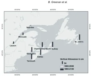
The hourly water level data for nine tide-gauge stations were downloaded from the Atlantic Zone Monitoring Program (AZMP) website (http://www.meds-sdmm.dfo-mpo.gc.ca/isdm-gdsi/azmp-pmza/sl-pm/index-eng.asp). The tide gauges measure sea level relative to land. The zero water levels at tide gauges are the local Canadian Hydrographic Service Chart Datum. These stations (Fig. 1) all have records of water levels longer than 25 years, which is needed for a satisfactory extremal analysis (Pugh 1996). The tide-gauge data are very useful for understanding present SLR and statistics of extreme water levels. In particular, the tide gauge stations in Charlottetown, Halifax and Saint John have century-long records of sea-level measurements (Table 1), providing a robust observational underpinning to the methodologies. It should be noted that the tide gauge in Saint John had siltation problems starting in 1980. The gauge was moved in 1999 and modified in 2006 (Greenberg et al. 2012).

Fig. 1 Map showing representative tide gauge stations in Atlantic Canada. Vertical allowances are shown in white for the period 1990–2050, and in black for the period 1990–2100. The scale of the black vertical bar in the legend is 54 cm.

Table 1 Summary of beginning year when tide-gauge stations were implemented, record length used for the extreme value analysis, location and scale parameters of the Gumbel distribution, and 50-year return level.

Stations Beginning

year Record length (year) Location parameter (cm) Scale parameter (cm) 50-year return level (cm)

Charlottetown 1911 87 152 16 213

Halifax 1895 94 134 10 172

North Sydney 1970 42 101 12 148

Quebec 1961 50 368 18 437

Rimouski 1984 27 265 10 304

Saint John 1896 96 428 11 470

Sept-Iles 1972 39 205 14 258

St. John’s 1935 58 109 8 141

Yarmouth 1956 46 261 10 303

Estimating sea-level allowances for Atlantic Canada under conditions of uncertain sea-level rise 19

PROJECTIONS OF RELATIVE SEA-LEVEL RISE

The derivation of the projections of relative sea-level rise in Atlantic Canada followed the methodology of Church et al. (2011) and Slangen et al. (2012), and is described in detail by Hunter et al. (2013, Appendix 1). The resultant projections are composed of terms due to: (1) the global-average sea-level rise which includes contributions due to thermal expansion, melting ice from glaciers and ice caps, Greenland and Antarctic ice sheets, and “scaled-up ice sheet discharge” (Meehl et al. 2007); (2) spatially-varying “fingerprints” to account for changes in the loading of the Earth and in the gravitational field, in response to ongoing changes in land ice (Mitrovica et al. 2001, 2011); (3) spatially-varying sea-level change due to change in ocean density and dynamics provided by atmosphere–ocean general circulation models (AOGCMS, Meehl et al. 2007); and (4) spatially-varying glacial isostatic adjustment (GIA) using the ICE-5G model (Peltier 2004) and modelling methodologies described by Kendall et al. (2005). GIA is the ongoing response of the Earth (solid surface motion and changes to the Earth’s gravitational field) to changes in surface loading caused by past changes in land ice, especially the deglaciation of the continental-scale ice sheets that commenced about 20 000 years ago.

Sea-level rise projections (5- and 95-percentile levels) were derived using the method described by Hunter et al. (2013) at 10-year intervals from 1990 to 2100 for the nine tide-gauge stations for the A1FI scenario (Neil White, CSIRO, pers. comm.), which is the IPCC SRES scenario providing the largest projected changes. In recent years, global climate trends have closely tracked the A1FI projections (Le Quéré et al. 2009). The scenario is now commonly used by decision-makers as the basis for responses to sea-level rise (Hunter 2012). Here we use the regional A1FI projections as the basis for deriving sea-level rise allowances in Atlantic Canada. While the global-average sea-level rise has been reported for six emission scenarios (B1, B2, A1B, A1T, A2, A1FI; Meehl et al. 2007), results from AOGCMs are only available for scenarios B1, A1B and A2, of which scenario A2 is the closest to A1FI. Therefore, the spatially-varying A1FI projections were derived from spatially-varying A2 projections which were scaled using ratios of global-average projections for A1FI and A2.

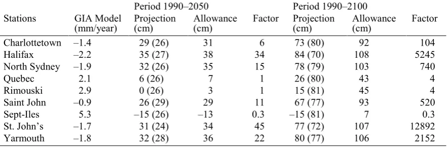
The GIA model projections in Atlantic Canada (Table 2, column 2) vary strongly spatially. It includes the effects of the redistribution of ocean water in response to gravitational changes and vertical land motion of the ocean floor (Kendall et al. 2005). Land subsidence of between –1 and –2 mm/year occurs at tide gauges along the coasts of Nova Scotia and the Gulf of Maine, whereas the land uplift is about 2 to 5 mm/year in the Gulf of St. Lawrence.

Table 2 Summary of GIA model predictions of vertical crustal motion and sea-level change, mean of the 5- and 95-percentile level of projections of sea-level rise (5- to 95-percentile range), allowances, and multiplying factors by which frequency of flooding events will increase with a sea-level rise of ∆z at tide-gauge stations.

Period 1990–2050 Period 1990–2100

Stations GIA Model

(mm/year) Projection (cm) Allowance (cm) Factor Projection (cm) Allowance (cm) Factor

Charlottetown –1.4 29 (26) 31 6 73 (80) 92 104

Halifax –2.2 35 (27) 38 34 84 (70) 108 5245

North Sydney –1.9 32 (26) 35 15 78 (79) 103 740

Quebec 2.1 6 (26) 7 1 26 (80) 43 4

Rimouski 2.9 0 (26) 3 1 15 (81) 45 4

Saint John –0.9 26 (29) 29 11 67 (77) 93 520

Sept-Iles 5.3 –15 (26) –13 0.3 –15 (81) 7 0.3

St. John’s –1.7 31 (24) 34 45 77 (72) 107 12892

Yarmouth –1.8 32 (28) 36 22 80 (77) 106 2152

level will rise between 26 to 35 cm in Scotian Shelf, Gulf of Maine and Newfoundland regions, and fall by 15 cm in Sept-Iles and remain approximately the same in the St. Lawrence Estuary for the period 1990–2050. The mean values of sea-level projections for the period 1990–2100 span from –15 to 84 cm. It is important to note that the uncertainty of the projections indicated by the 5- to 95-percentile range increases with time, and is comparable to the central values.

REGIONAL SEA-LEVEL ALLOWANCES

Following Hunter (2012), the results are presented in two different ways. Firstly, a rise of mean sea level ∆𝑧𝑧 increases the expected number of exceedences N, or reduces the return period by a factor of exp∆𝑧𝑧_𝜆𝜆, which is determined by combined effect of the Gumbel scale parameter and the mean sea-level rise. In other words, the fixed level is flooded exp∆𝑧𝑧_𝜆𝜆 more times when the mean sea level is raised by ∆𝑧𝑧.

This factor (Table 2) shows significant spatial variation for Atlantic Canada with a range of 0.3 to 45 for the period 1990–2050. The largest values of this multiplying factor are in St. John’s Newfoundland, coinciding with the smallest value of the scale parameter. The factors are small in St. Lawrence Estuary and the northern Gulf of St. Lawrence, due to a small sea-level rise and sea- level fall, respectively. While the mean sea-level rise is similar for Charlottetown and St. John’s, the multiplying factor depends only on the spatially-varying scale parameter, and shows a large difference between the two stations, being 6 and 45, respectively.

In comparison with the period 1990–2100, the number of flooding events (Table 2) will increase by a factor of 104–12892 on the Scotian Shelf, Gulf of Maine and Newfoundland, increase slightly by a factor of 4 in St. Lawrence Estuary and decrease in the northern Gulf of St. Lawrence. One way to interpret the factor of exp∆𝑧𝑧_𝜆𝜆 is that a flooding event that occurred on average every R years in the past will occur every 𝑅𝑅/exp∆𝑧𝑧_𝜆𝜆 years. For example, in St. John’s, a 50-year flooding event in the past will become an annual flooding event for the period 1990–2050 (50/45 = 1 year), and will occur every day for the period 1990–2100 (50 × 365/12892 = 1.4 day).

The other way of presenting the results is in terms of the sea-level rise allowances for a normal uncertainty distribution. The allowance is composed of two parts: the mean sea-level rise (∆𝑧𝑧) and the term 𝜎𝜎_2𝜆𝜆2 arising from the uncertainty in future sea-level rise. For the A1FI emission scenario and the period 1990–2050, the allowance (Table 2) ranges from –13 to 38 cm and is slightly greater than the mean projections of sea-level rise by 1–4 cm. For comparison, Table 2 shows that the allowance for the period 1990–2100 ranges from 7 to 108 cm and is much larger than the corresponding mean projection by 17–30 cm. This increase in the difference between the allowance and the mean projection lies in the increasing uncertainty of sea-level projections with time. The allowances for different periods are always within the 95-percentile upper limit of regional sea-level projections at all tide-gauge stations.

The sea-level allowance also shows a significant spatial variation (Fig. 1), largely affected by spatially-varying projections of sea-level rise. The allowances range from 29 to 38 cm (77 to 84 cm) at sites along the coast of Nova Scotia and Newfoundland for the period 1990–2050 (1990–2100). Sites in the Gulf of St. Lawrence have negative or small positive allowances, spanning from –13 to 7 cm (–15 to 26 cm) for the period 1990–2050 (1990–2100).

CONCLUSIONS

Estimating sea-level allowances for Atlantic Canada under conditions of uncertain sea-level rise 21

GIA and fingerprints. For the A1FI emission scenario and for the period of 1990–2050, the sea-level is most likely to rise between 26 and 35 cm at sites in the Scotian Shelf, Gulf of Maine and Newfoundland regions, to rise between 0 and 6 cm at sites in St. Lawrence Estuary, and to fall by 15 cm at sites in the northern Gulf of St. Lawrence. It should be emphasized that these are only based on the results from the nine tide gauge sites considered herein and so the range of factors for the region could be larger than stated here.

In most regions of Atlantic Canada, new infrastructure will need to be built higher to account for future sea-level rise. An attractive feature of this allowance is that it does not require that the expected number of exceedences be prescribed. The range of future allowances for 1990–2050 is between –13 and 38 cm, while the range for 1990–2100 is between 7 and 108 cm at tide-gauge sites. In the Bay of Fundy and Gulf of Maine, the vertical allowances in this region should also take account of the potential change in tidal amplitude (Greenberg et al. 2012).

Acknowledgements This work is funded by the DFO Aquatic Climate Change Adaptation Services Program (ACCASP). We would like to thank all those who participated in the 18 October 2012 workshop held at Bedford Institute of Oceanography. This is an output of the NRCan Climate Change Geoscience Program. Support from the NRCan Climate Change Impacts and Adaptation Division is gratefully acknowledged by Thomas S. James.

REFERENCES

Bernier, N. B. and Thompson K. R. (2006) Predicting the frequency of storm surges and extreme sea levels in the northwest Atlantic J. Geophys. Res., 111, C10009, doi:10.1029/2005JC003168.

Church, J. A., et al. (2011) Understanding and projecting sea level change. Oceanography 24(2), 130–143, doi:10.5670/oceanog.2011.33.

Coles, S. (2001) An Introduction to Statistical Modeling of Extreme Values. London, Berlin, Heidelberg: Springer-Verlag. Forbes, D. L., et al. (2009) Halifax Harbour extreme water levels in the context of climate change: scenarios for a 100-year

planning horizon, Geological Survey of Canada, Open File 6346, iv+22 p.

Greenberg D. A., et al. (2012) Climate change, mean sea level and high tides in the Bay of Fundy. Atmosphere–Ocean

doi:10.1080/07055900.2012.668670.

Hunter, J. (2012) A simple technique for estimating an allowance for uncertain sea-level rise. Climatic Change 113, 239–252, DOI 10.1007/s10584-011-0332-1.

Hunter, J., et al. (2013) Towards a global regionally-varying allowance for sea-level rise. Ocean Engineering

doi:10.1016/j.oceaneng.2012.12.041.

James, T. S., et al. (2011) Sea-level Projections for five pilot communities of the Nunavut Climate Change Partnership; Geological Survey of Canada, Open File 6715, 23 p.

Kendall, R., Mitrovica, J. and Milne, G. (2005) On post-glacial sea level – II. Numerical formulation and comparative results on spherically symmetric models. Geophysical Journal International 161(3), 679–706, doi:10.1111/j.1365-246X.2005.02553.x.

Meehl, G., et al. (2007) Climate Change 2007: The Physical Science Basis. Contribution of Working Group I to the Fourth Assessment Report of the Intergovernmental Panel on Climate Change, Cambridge University Press, Cambridge, United Kingdom and New York, NY, USA, chap. 10, pp 747–845.

Mitrovica J. et al. (2001) Recent mass balance of polar ice sheets inferred from patterns of global sea-level change. Nature

409(6823), 1026–1029, doi 10.1038/35059054.

Mitrovica, J., et al. (2011) On the robustness of predictions of sea level fingerprints. Geophysical Journal International 187, 729–742, doi 10.1111/j.1365-246X.2011.05090.x.

Peltier, W. (2004) Global glacial isostasy and the surface of the ice-age earth: the ICE-5G (VM2) model and GRACE. Ann. Rev Earth Planet Sci. 32, 111–149.

Pugh, D. (1996) Tides, Surges and Mean Sea-Level. John Wiley & Sons, reprinted with corrections, http://eprints.soton.ac.uk/19157/01/sealevel.pdf, Chichester, New York, Brisbane, Toronto and Singapore.

Ranasinghe, R., et al. (2012) Climate-change impact assessment for inlet-interrupted coastlines. Nature, doi: 10.1038/nclimate1664.

Slangen, A., et al. (2011) Towards regional projections of twenty-first century sea-level change based on IPCC SRES scenarios.

Climate Dynamics, doi:10.1007/s00382-011-1057-6.

Zhai, L., et al. (2013) Estimating sea-level allowances for Atlantic Canada under conditions of uncertain sea-level rise.