University of Pennsylvania
ScholarlyCommons
Publicly Accessible Penn Dissertations
2017
Managing Self-Scheduling Capacity
Kaitlin Marie Daniels
University of Pennsylvania, [email protected]
Follow this and additional works at:
https://repository.upenn.edu/edissertations
Part of the
Operational Research Commons
This paper is posted at ScholarlyCommons.https://repository.upenn.edu/edissertations/3065
For more information, please [email protected].
Recommended Citation
Daniels, Kaitlin Marie, "Managing Self-Scheduling Capacity" (2017).Publicly Accessible Penn Dissertations. 3065.
Managing Self-Scheduling Capacity
Abstract
Gig-economy platform like Uber, Lyft, Postmates, and Instacart have created markets in which independent service providers provide on-demand service to consumers. A hallmark of this arrangement is that providers decide for themselves when, where, and how much to work. In other words, the platform does not set its capacity's schedule; instead its capacity "self-schedules." This decentralization of decision making can create value for providers. The platform's challenge is then to devise a contract with its capacity that allows it to capture some of this value. I study the platform's contracting problem in three chapters. In the first, I show that the platform can benefit from allowing its providers to self-schedule. In the second, I study the platform's strategy when coordinating supply and demand across multiple states of the world. I show that the resulting dynamic pricing policy can be beneficial to consumers, despite widespread dislike of the real-world practice. I also show that, in many cases, the platform need not independently vary payments to providers to achieve near-optimal profit. Instead the platform may pay its providers a fixed percent commission on the price paid by consumers per completed service. In the final chapter, I argue that the findings above are distinct from the traditional two-sided markets literature. Though a classic two-sided market model experiences near-optimal performance of the fixed commission in many cases, the market conditions that produce poor fixed
commission performance differ between the gig-economy model and the two-sided markets model. Because the two-sided market model does not accurately predict poor gig-economy fixed commission performance, it is important to study a model tailored the gig-economy to understand gig-economy specific applications.
Degree Type
Dissertation
Degree Name
Doctor of Philosophy (PhD)
Graduate Group
Operations & Information Management
First Advisor
Gerard P. Cachon
Keywords
contract design, gig-economy, self-scheduling capacity, service operations, sharing-economy, Uber
Subject Categories
MANAGING SELF-SCHEDULING CAPACITY
Kaitlin M. Daniels
A DISSERTATION
in
Operations, Information and Decisions
For the Graduate Group in Managerial Science and Applied Economics
Presented to the Faculties of the University of Pennsylvania
in
Partial Fulfillment of the Requirements for the
Degree of Doctor of Philosophy
2017
Supervisor of Dissertation
Gerard P. Cachon, Professor of Operations, Information and Decisions
Graduate Group Chairperson
Catherine Schrand, Celia Z. Moh Professor, Professor of Accounting
Dissertation Committee
Noah Gans, Professor of Operations, Information and Decisions Ruben Lobel, Data Scientist, Airbnb
Xuanming Su, Professor of Operations, Information and Decisions
MANAGING SELF-SCHEDULING CAPACITY
c
COPYRIGHT
2017
Kaitlin Marie Daniels
This work is licensed under the Creative Commons Attribution NonCommercial-ShareAlike 3.0 License
To view a copy of this license, visit
ACKNOWLEDGEMENT
ABSTRACT
MANAGING SELF-SCHEDULING CAPACITY
Kaitlin M. Daniels
Gerard P. Cachon
TABLE OF CONTENTS
ACKNOWLEDGEMENT . . . iii
ABSTRACT . . . iv
LIST OF TABLES . . . vii
LIST OF ILLUSTRATIONS . . . viii
PREFACE . . . ix
CHAPTER 1 : Demand Response in Electricity Markets: Voluntary and Automated Curtailment Contracts . . . 1
1.1 Introduction . . . 1
1.2 Literature Review . . . 5
1.3 Consumer Behavior . . . 8
1.4 Firm’s Contract Choice . . . 10
1.5 System Welfare and Environmental Impact . . . 14
1.6 Optimal Curtailment Contracts . . . 16
1.7 Numerical Results . . . 19
1.8 Conclusion . . . 21
CHAPTER 2 : The Role of Surge Pricing on a Service Platform with Self-Scheduling Capacity . . . 24
2.1 Introduction . . . 24
2.2 Literature Review . . . 28
2.3 Model . . . 30
2.4 Contract Design . . . 35
2.6 Numerical Study . . . 44
2.7 Self-Scheduling vs. Central-Scheduling of Capacity . . . 52
2.8 Discussion . . . 54
2.9 Conclusion . . . 55
CHAPTER 3 : Distinguishing the Gig-Economy from Two-Sided Markets . . . 58
3.1 Introduction . . . 58
3.2 Model . . . 62
3.3 Gig Economy . . . 65
3.4 Two-Sided Markets . . . 67
3.5 Numerical Analysis . . . 70
3.6 Conclusion . . . 74
APPENDIX . . . 75
LIST OF TABLES
TABLE 1 : Linear Contract Parameters . . . 11
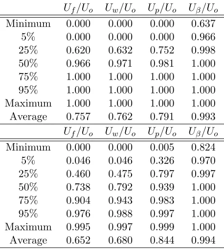
TABLE 2 : Tested parameter values. All combinations of these values constitute 14,700 scenarios. . . 45 TABLE 3 : Frequency of different versions of the fixed contract. . . 46 TABLE 4 : Relative Profitability of Suboptimal Contracts. Profit performance
of the four suboptimal contracts relative to the optimal contract in all 14,700 scenarios (left table) and in the 2,253 scenarios in which the fixed contract serves both demand states (right table). The subscripts f, w, p, β, and o to refer to the fixed, dynamic wage, dynamic price, commission and optimal contracts, respectively. . . 47 TABLE 5 : Relative Consumer Surplus with Poor Utilization. The ratio of
con-sumer surplus and number of providers with the dynamic wage, dy-namic price, commission or optimal contract to the fixed contract in the 591 scenarios with poor utilization. . . 50 TABLE 6 : Relative Consumer Surplus with Poor Service. The ratio of
con-sumer surplus and number of providers with the dynamic wage, dy-namic price, commission or optimal contract to the fixed contract in the 1,662 scenarios with poor service. . . 51
LIST OF ILLUSTRATIONS
FIGURE 1 : Structure of the Market with Curtailment Contracts . . . 4 FIGURE 2 : This figure illustrates the firm’s and the social planner’s contract
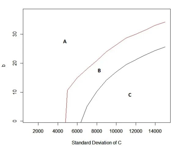
choices as functions of market price sensitivity and cost variance. In Region A ΠLA≥ΠLV and WAL≥WVL, in Region B ΠLA≥ΠLV but
WVL≥WAL, and in Region C ΠLV ≥ΠLA andWVL≥WAL. . . 15 FIGURE 3 : A comparison of contract performance for the firm’s profit . . . . 20 FIGURE 4 : A comparison of contract performance for the social welfare. . . . 21
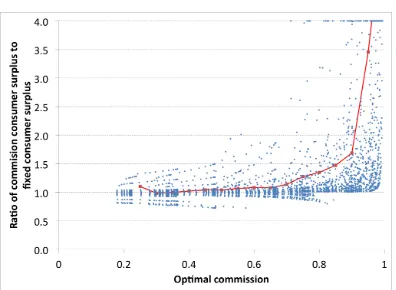
FIGURE 5 : Timeline of events . . . 30 FIGURE 6 : An example of demand and capacity rationing with a fixed contract. 36 FIGURE 7 : Relative Consumer Surplus as a Function of Commission. The ratio
of consumer surplus with the commission contract to consumer sur-plus with the fixed contract as a function of the commission earned by providers with the commission contract in the 2,253 scenarios in which the fixed contract serves both demand states. Squares indicate the average ratio for scenarios grouped by the commission contract commission in 0.05 intervals. . . 52
FIGURE 8 : Illustrative plots. All plots have µg = 1, CVg = .5, and CVf =
PREFACE
Here I study markets in which a firm relies on capacity to provide a good or service that it does not directly control. This capacity is the aggregation of individual producers or service providers who produce/serve according to their own self-interest. These individuals face non-trivial, non-constant, and private opportunity costs for the time spent produc-ing/serving through the firm, so each individual only provides capacity to the firm if his earnings from doing so exceed his opportunity cost. In other words, the firm does not set its capacity’s service/production schedule, instead its capacity “self-schedules.”
Self-scheduling arrangements are most associated with the on-demand service industry com-monly known as the gig-economy. Gig-economy firms serve as platforms that connect customers with self-scheduling service providers. Noteworthy examples include the ride-sharing platforms Uber and Lyft, the delivery platforms Postmates and Instacart, and the on-demand labor platforms TaskRabbit and Bellhops. According to Farrell and Greig (2016), between 2012 and 2015 the fraction of JPMorgan Chase account holders receiving monthly income from participation in the gig-economy grew 10-fold, constituting 1% of ac-count holders in 2015. Furthermore, the proportion of acac-count-holders having ever received income from participation in the gig-economy grew 47-fold, indicating that 4.2% of account holders worked a gig at some point during that time period (Farrell and Greig, 2016).
Providers report that their primary attraction to the gig-economy is their ability to self-schedule. A recent Benenson Strategy Group survey of Uber drivers reports that 87% of respondents partner with Uber “to be my own boss and set my own schedule” (Hall and Krueger, 2015a). The key consequence of this framework is that decentralization decision making can create value for providers. However, it does not immediately follow that this arrangement also benefits the platform or consumers.
arrangement. Second I derive a firm’s profit optimal dynamic pricing contract and de-termine its effect on consumer welfare. Finally, I illustrate the differences between the gig-economy and the traditional two-sided markets literature.
The first chapter is motivated by a setting with self-scheduling capacity that existed long before the gig-economy: the electricity market. “Curtailment contracts” in electricity mar-kets allow a firm to pay electricity consumersnot to use electricity and to sell this foregone consumption as “virtual” generation on the electricity market. In the firm’s contract with electricity consumers, it may either allow consumers to curtail their consumption as they wish (i.e. self-schedule) or it may require consumer to commit to a level of curtailment. In this context, the firm evaluates the profitability of self-scheduling in a market where the firm is a price taker and price decreases in the production of the firm. I find that the firm generally prefers self-scheduling when consumers face sufficiently varied opportunity costs and when the slope of the price curve is sufficiently small.
The second chapter is motivated by the dynamic pricing strategies used by some gig-economy firms (most notably Uber’s “Surge Pricing”). The firm chooses a pricing strategy to coordinate its self-scheduling capacity with variable demand. The firm’s profit maximiz-ing incentive structure charges consumers a demand-contmaximiz-ingent price and offers providers a demand-contingent wage. I consider the profit and consumer surplus implications of restrict-ing prices to be constant across all demand regimes and, alternatively, allowrestrict-ing demand-contingent prices but restricting wages to be a fixed percentage of prices (i.e. providers earn a fixed commission). I find that while restricting the firm to a fixed price causes significant profit loss for the firm, requiring a fixed commission generally produces near-optimal profit. I further demonstrate that consumers can benefit from demand-contingent prices due to depressed prices in low demand regimes and expanded access to service in high demand regimes.
platform happens on a much longer time scale than in the gig-economy, so the classic models ignore capacity constraints that are very relevant to the operations of the gig-economy. For example, a retailer chooses to accept American Express based on the volume of customers that carry American Express. In contrast, an Uber driver can only serve one customer at a time, so even if there are many customers demanding rides at the same time, the Uber driver only cares that he is assured a passenger. I find that these difference lead the two models to make significantly different predictions. In particular, I focus on the profitability of a fixed commission in each setting. I show that though a classic two-sided market model experiences near-optimal performance of the fixed commission in many cases, the market conditions that produce poor fixed commission performance differ between the gig-economy model and the two-sided markets model. Because the two-sided market model does not accurately predict poor gig-economy fixed commission performance, it is important to study a model tailored the gig-economy to understand gig-economy specific applications.
CHAPTER 1 : Demand Response in Electricity Markets: Voluntary and
Automated Curtailment Contracts
1.1. Introduction
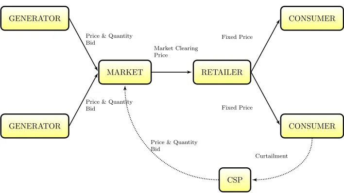
Electricity markets today suffer from a fundamental flaw: consumption does not respond to market signals. This is a result of the organization of the electricity supply chain, as illustrated in Figure 1. Conventional generators submit a menu of prices and production levels to the market’s clearinghouse, the Independent System Operator (ISO). The ISO constructs the market supply curve by ordering these bids from least to most expensive per kilowatt hour (kWh). Market demand determines the price at which all consumption is purchased, which is known as a uniform-price auction. However, consumers do not satisfy their demand by purchasing electricity on the market themselves. Instead, consumers are served by local utilities and other electricity retailers that buy on the market at the market price and sell to consumers at a fixed fee per kWh. Though the market price varies, end-consumers only experience their fixed fee, even in times of peak load. As a result, end-consumers that would otherwise be priced out of the market continue to consume, and demand can creep dangerously close to the system’s limit, threatening black- and brown-outs.
2011 the Federal Energy Regulatory Commission mandated that foregone end-consumption be treated as conventional generation during peak load events, meaning the extra supply created by curtailed consumption can be sold on the market for the full market price.1 In the next 5 years curtailment contracts, along with other demand response efforts, are projected to decrease peak demand by more than 4% 1 In the next 5 years curtailment contracts, along with other demand response efforts, are projected to decrease peak demand by more than 4%.2.
When a consumer curtails his consumption, he incurs an opportunity cost which varies based on the value of his initial consumption. For example, a residential consumer’s value of air conditioning is increasing in the ambient temperature, so his opportunity cost from curtailing his electricity is higher during a heat wave than on a normal summer day. Under a curtailment contract, the CSP calls upon contracted consumers to reduce their consumption when market conditions make selling virtual load a profitable endeavor. Typically, the CSP participates the electricity market during peak load events, caused by extreme demand or generation outages. Because consumers do not anticipate peak load events, the value of the curtailed consumption is uncertain ex ante. Furthermore, a consumer’s value of consumption is private information.
Curtailment contracts can be partitioned into two classes. Traditionally consumers relin-quish control over their curtailment decisions, allowing the CSP to remotely adjust their consumption during peak load events. We will call this an automated curtailment contract. The curtailment amount automatically imposed by the CSP is determined by the consumer in advance of any particular peak load event. Therefore, curtailment under an automated contract is determined in expectation of the consumer’s value of consumption at the time of curtailment. Technological advances in smart metering have introduced a new generation of curtailment contracts which we will call voluntary. Under the voluntary contract con-sumers decide the level of curtailment provided to the CSP at the time of the peak event.
1
FERC Order 745 - http://www.ferc.gov/EventCalendar/Files/20110315105757-RM10-17-000.pdf
The voluntary contract, therefore, allows consumers to make curtailment decisions with full knowledge of their cost.
In this paper, we study a CSP’s choice of contract class to offer a set of consumers. In practice, CSPs offer distinct contracts to different customer segments (e.g. residential, commercial). A contract is designed for a particular subset of consumers who have similar attributes. We assume that the consumers within this subset have a homogeneous value distribution of electricity consumption. For example, interior heating and cooling represents nearly a third of the residential electricity consumption in the United States 3. The value of this consumption varies as a function of temperature, which affects consumers in the same geographic area equally.
The CSP’s choice between automated and voluntary contracts echoes the trend in the service industry toward allowing service providers to self-schedule. Just as firms like Uber allow service providers to choose when and how much to work, a voluntary curtailment contract allows consumers to choose whether and how much to curtail their loads. Like electricity consumers curtailing their loads, self-scheduling service providers encounter an opportunity cost when they offer their services. The burgeoning operations literature on this topic considers providers with independent and identically distributed opportunity costs (e.g. Cachon et al. (2017), Gurvich et al. (2015), Ibrahim and Arifoglu (2015)). Curtailment contracts offer an appropriate application to extend this literature by studying a self-scheduling environment in which opportunity costs are correlated.
MARKET GENERATOR
GENERATOR
RETAILER
CONSUMER
CONSUMER
CSP Price & Quantity
Bid
Price & Quantity Bid
Market Clearing Price
Fixed Price
Fixed Price
Curtailment Price & Quantity
Bid
Figure 1: Structure of the Market with Curtailment Contracts
cost distribution, the firm’s contract decision is driven simply by the variance of cost. This application also allows us to measure the environmental effect of the CSP’s contract choice. While the profit maximizing CSP contract choice also maximizes the positive environmental impact of demand response, the incentives of the CSP and a welfare maximizing social planner are not aligned. We characterize the market and customer conditions that create this misalignment, those in which a social planner should encourage voluntary contracts even though the CSP would rather adopt the automated contract.
1.2. Literature Review
The management of non-storable goods with periodic demand, such as electricity, has long been of interest to economists. The peak load pricing literature studies capacity and pricing decisions made by a firm facing demand that periodically shifts from low to high. For a thorough review please see Crew et al. (1995). When demand is stochastic, a firm with finite capacity faces a non-zero probability that its supply will be insufficient to satisfy demand during peak load events. In the electricity setting this means that a utility will interrupt its service to a fraction of its customers. To efficiently allocate its electricity, a utility may segment the service it provides based on the reliability of the service. Many papers have been dedicated to characterizing the optimal menu of price and reliability contracts to offer under this service differentiation based on reliability. See Chao and Wilson (1987), Marchand (1974), Chao et al. (1986), Smith (1989), Oren and Doucet (1990), and Oren and Smith (1992). These contracts are the direct ancestors of the automated curtailment contracts studied in this paper. Both sets of contracts allow utilities to reduce demand to address insufficient supply. However, the incentives facing the firm in our model differ from those listed above. Previous papers have considered contracts that maximize social welfare. In contrast, our model incorporates the monetary incentives for efficient demand-side management, so our firm is purely a profit maximizer. Furthermore, previous models have assumed service delivery to be binary; a consumer’s electricity needs are either met or not. The ubiquity of smart meters today makes the question of how much electricity to curtail from a consumer both relevant and important. We incorporate this dimension by including a continuous load curtailment decision variable.
interaction with consumers resembles the curtailment contracts studied in our model. As in our model, Iyer et al. (2003) must remunerate consumers in return for their participation in the demand management program. However, unlike our model the authors do not allow the supplier to determine how best to reward consumer participation. Their reimbursement is linear and exogenous.
Our work is born of a rich literature studying demand-side management. Our key inno-vation is the introduction of the voluntary curtailment contracts and the characterization of when it should be preferred over the automated type. Both the reliability-based service differentiation literature and Iyer et al. (2003) assume that all demand management uses contracts that we consider “automated.” Specifically, service reliability is determined before service interruption and interruption is controlled by the firm. Similarly, the engineering literature on demand response has primarily focused on how to optimally activate a portfo-lio of automated load curtailment customers (see for example Goyal et al. 2013 and Taylor and Mathieu 2014). Wu and Kapuscinski (2013) show how curtailment of intermittent generation can also benefit the system by reducing uncertainty for conventional generation sources. While under reliability-based service contracts consumers may sort themselves effi-ciently given their ex-ante understanding of their value for electricity, we expect consumers to have a better understanding of their valuation at the time they wish to consume electric-ity. The automated structure affords consumers no flexibility at the time of consumption. Allowing consumers to adjust their service curtailment based on new information at the time of consumption certainly generates extra value for consumers. In the analysis that follows we will show when that extra value can also benefit the firm.
as in Eppen and Iyer (1997) and quantity flexible contracts as in Tsay and Lovejoy (1999)). Barnes-Schuster et al. (2002) show that these contracts are special cases of a larger problem in which the firm can purchase options from a supplier at a specified exercise price. The resulting chain coordinating contract is a piece-wise linear exercise price. However, flexibility is not necessarily profit improving when suppliers are not forced to comply with capacity requests from a manufacturer who has private information about demand. Cachon and Lariviere (2001) show that a manufacturer inducing capacity investment in a supplier, based on asymmetric information about demand, must perform a costly act (increase capacity requested or committed order size, lump sum transfer) to induce the appropriate capacity investment in the supplier. Similarly, suppliers in our chain are not forced to comply with capacity requests under the voluntary contract. In the analysis that follows we will show when supply flexibility is beneficial to the firm and when the firm is better off enforcing compliance.
sac-rifice reliability to achieve lower procurement cost or to allocate risk appropriately. Tomlin (2006) studies how the characteristics of the unreliable source, in terms of % uptime and expected disruption length, determine a firm’s choice between a reliable and an unreliable source with fixed procurement costs. Yang et al. (2009) investigates a firm’s willingness to pay for reliability information when a supplier’s reliability is private information. Similarly, Wang et al. (2010), Kim (2011), and Liu et al. (2010) explore a firm’s decision to invest in endeavors that will improve the reliability of its supplier. This parallels the premium we show that the firm pays to consumers under an automated contract.
1.3. Consumer Behavior
In this section we describe the behavior of a customer who has decided to participate in a contract offered by the CSP, henceforth referred to as the firm. Suppose the firm has an exogenously determined number of consumers, N, who are enrolled in the firm’s curtailment contract. Each consumer will be called upon by the firm during peak load events to reduce his energy consumption in return for payment. We would like to emphasize that the dynamics of our model are the opposite of a conventional supply chain; here the firm buys from the consumer to sell on the market instead of the other way around. In most applications the firm contracts with a pool of consumers. We characterize the time until the next event as a single period. We assume that consumers have a baseline value of curtailment, q, defined by
V(q) =−Cq2
sea-son than during an off seasea-son, and residential consumers all increasingly value their ability to turn on their air conditioners the hotter the weather is. Hence we assume that consumers are homogeneous in the value coefficient,C, and that this value coefficient varies over time. Under a curtailment contract, the firm offers each consumer incentives to alter his con-sumption pattern. These incentives are offered in response to peak load events, which we assume consumers do not predict. Furthermore, the firm does not observeC, so from both firm and consumer point of view, this quantity is uncertain. We therefore define C to be a random variable, with density g, distribution G and finite support{CL, CH}. In our model both the firm and consumers have full knowledge of the distribution of C. Whether the consumers decide their actual curtailment with full knowledge of C distinguishes the two contracts studied in this paper.
1.3.1. Linear Automated Contracts
Under the automated contract the firm offers a linear payment,w, per unit of the consumer’s load curtailment. The
firm also offers a fixed transfer per transaction,f, which may be positive or negative. When
f = 0 the firm simply offers a wholesale price contract. A consumer’s corresponding value function is
VA(q) =E[wq−Cq2+f1{q >0}].
Given knowledge of (w, f) a consumer chooses to participate in the contract and must specify the load reduction quantity,qAthat he will provide to the
his value given the payment structure:
qA= argmaxVA(q) =
w
2E[C].
1.3.2. Linear Voluntary Contracts
In contrast with the automated contract, under the voluntary contract each consumer learns the realization of C before choosing their curtailment. A consumer’s corresponding value function is
VV(q)−wq−Cq2+f1{q >0}.
In response to the firm’s offered payment, (w, f), each consumer chooses his curtailment to maximize his value:
qv = argmaxVV(q) = 1 2C.
1.4. Firm’s Contract Choice
Given the consumer behavior described above, the
firm wishes to maximize her expected profit. Under a given contract type, the lever at her disposal is the payment level (w, f). By reducing either w or f the firm lowers her cost. However, the
market will not be large enough to demonstrate higher order effects, we approximate the market price curve asP(q) =a−bq. Letqij denote consumeri’s curtailment under contract type j. We can characterize the firm’s expected profit under contract type j as
max wj,fj
Π(wj, fj) =E
"
P
N
X
i=1
qji
! N X
i=1
qji− N
X
i=1
wjqij−fj
#
s.t.Vj(qij)≥0∀i.
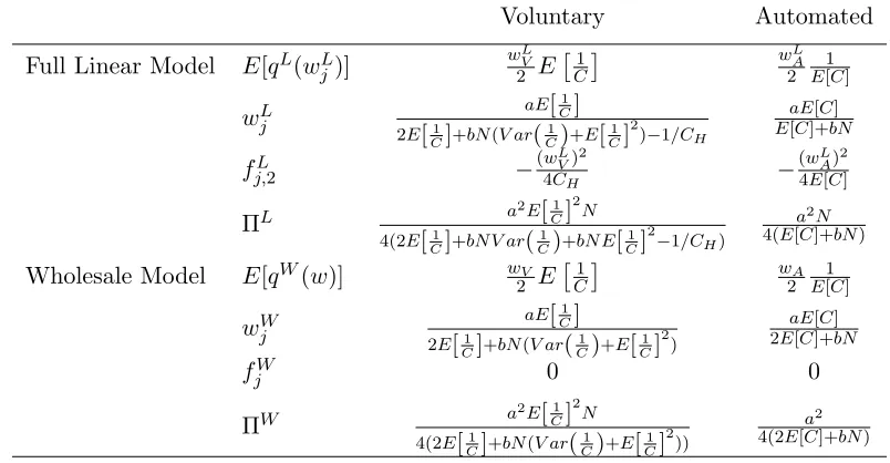
Note that qji(wj, fj) is independent offj . As a result the firm usesfA to extract all of the expected consumer surplus under the automated contract. However, because the consumer decides to participate after observing his cost under the voluntary contract, the voluntary contract only extracts all consumer surplus if the consumer’s cost achieves its highest value. The optimal payments and profits are summarized in Table 1.
Table 1: Linear Contract Parameters
Voluntary Automated
Full Linear Model E[qL(wjL)] wVL
2 E
1
C
wLA
2 1 E[C]
wLj aE[
1
C]
2E[1
C]+bN(V ar(
1
C)+E[
1
C]
2 )−1/CH
aE[C] E[C]+bN
fj,L2 −(wLV)
2
4CH −
(wAL)2 4E[C]
ΠL a
2E[1
C]
2 N
4(2E[1
C]+bN V ar(
1
C)+bN E[
1
C]
2
−1/CH)
a2N 4(E[C]+bN)
Wholesale Model E[qW(w)] wV
2 E 1 C wA 2 1 E[C]
wWj aE[
1
C]
2E[1
C]+bN(V ar(
1
C)+E[
1
C]
2 )
aE[C] 2E[C]+bN
fjW 0 0
ΠW a
2E[1
C]
2 N
4(2E[1
C]+bN(V ar(
1
C)+E[
1
C]
2 ))
a2 4(2E[C]+bN)
In Table 1 we use the superscriptL to denote quantities under the optimal contract where the fixed payment is non-zero. This is to differentiate from the special case where the fixed payment is zero, which we refer to as the wholesale contract and denote with the superscript
givenwj andfj under the voluntary contract is at least as large as the load reduction under the automated. This follows from Jensen’s inequality which requires
E[1
C]≥
1
E[C].
By Jensen’s inequality we see that the optimal unit payment wLj is no larger under the voluntary than under the automated. These two rows confirm that the voluntary contract has option value to consumers. Consumers are willing to accept smaller payments for the same load provided to the firm in exchange for the flexibility of the voluntary contract. In other words, the firm must pay a premium for a certain (reliable) supply of curtailment. We include in Table 1 the special case wholesale contract where fjW = 0 as a reference for future analysis. While many contracts currently in use follow this format, it is easy to see that ΠLj ≥ ΠWj for either the voluntary or the automated. We will focus our analysis on the two-part linear payment scheme (denoted by the superscript L), returning to use the wholesale contract as a benchmark in the numerical experiments of Section 7. Of primary interest is the fourth row in Table 1. This row describes the expected optimal profit under the voluntary and automated contracts respectively. The difference between voluntary and automated contract profit is
ΠV −ΠA=E[C]− 2
E[1/C]+ 1
CHE[1/C]
−bN c2v (1.1)
voluntary contract also causes variance in the total load curtailed, which affects the market price faced by the firm. We can conclude from (1.1) that in sufficiently sensitive markets the risk of low market price from the variance in load curtailed under the voluntary contract hurts expected revenue more than the gains from paying consumers less. Similarly, the more consumers the firm contracts, the larger the impact variance has on the load curtailed under the voluntary contract. In choosing between these contracts, the firm weighs this price risk against the lower wages per unit curtailment achieved under the voluntary contract.
To understand the role of the consumer’s distribution of C on contract performance, we must disentangle three statistics: E[C], E[1/C], and V ar(1/C). Fixing the average cost
E[C], we show in Theorem 1 the choice of contract depends on the Jensen Gap, which is the slackness of the Jensen inequality,E[1/C]−1/E[C].
Theorem 1. For a givenE[C]there exists y¯≥z¯such that
1. for all EC1≥y¯, ΠLA≤ΠLV 2. for all E1
C
≤z¯, ΠL
A≥ΠLV.
For a fixedE[C] decreasingE[1/C] decreases the Jensen Gap: a sufficiently small Jensen’s Gap favors the automated contract and a sufficiently large Jensen’s Gap favors the voluntary contract. Notice that the Jensen Gap is the difference in expected curtailment under the voluntary and automated contracts for a given unit payment. The larger this difference, the larger the payment required by the automated contract to obtain the same curtailment as the voluntary. At some point, the voluntary contract allows the firm to offer a small enough payment that the cost savings under the voluntary contract outweigh the price risk the firm must bear.
Theorem 2. For symmetric distribution G with a given mean, increasing the variance of
C increases the Jensen Gap.
partially internalizes this value through its per transaction fee, fV, causing firms to prefer voluntary contracts for sufficiently varied distributions ofC.
1.5. System Welfare and Environmental Impact
In this section, we will consider the contract choice decision from the perspective of an integrated system. Instead of maximizing profit, the centralized decision maker’s objective is to maximize system welfare, i.e. the sum of the consumer and firm surplus. Transfers between entities are no longer considered, so system welfare may be expressed as
Wj =E
"
a−b
N
X
i=1
qij
! N X
i=1
qij−CsumNi=1(qij)2
#
.
Using Table 1 yields:
WA=
a2N
4(E[C] +bN)
WV =
q2E[1/c]2N
2(2E[1/C] +bN E[1/C2]−1/C H)
− a
2E[1/C]2N(bN E[1/C2] +E[1/C]) 4(2E[1/C] +bN E[1/C2]−1/C
H)
Note that the firm extracts all consumer surplus under the automated contract so WAL = ΠLA.. We can show, however, that welfare under the voluntary contract exceeds the value of the firm’s profit. This demonstrates that consumers benefit from the flexibility of the voluntary contract. From this fact we derive the following theorem.
Theorem 3. 1. If ΠLV ≥ΠLA, then WV ≥WA.
2. If WA≥WV, then ΠLA≥ΠLV.
voluntary contract in response to low market price sensitivity and high cost uncertainty. However, in Region B the firm chooses an automated contract where the central planner prefers the voluntary contract. We conclude that a regulator may be inclined to encourage the voluntary contract in markets where the ratio of price sensitivity and cost uncertainty is not sufficient for the firm to adopt this contract.
Figure 2: This figure illustrates the firm’s and the social planner’s contract choices as functions of market price sensitivity and cost variance. In Region A ΠLA≥ΠLV and WAL≥
WVL, in Region B ΠLA≥ΠLV butWVL≥WAL, and in Region C ΠLV ≥ΠLA and WVL≥WAL.
From an environmental perspective, consider a regulator whose objective is to minimize energy consumption, which is to maximize the total load reduction delivered by the cur-tailment contract. As shown in the following theorem, in this case the firm and the social planner prefer the same contract.
Theorem 4. ΠLV ≥ΠLA if and only if E[qVL]≥E[qLA].
social planner’s incentives are aligned with those of a profit maximizing firm’s.
1.6. Optimal Curtailment Contracts
We have thus far assumed that the firm is restricted to paying the consumer linearly. While this is a common contract structure, we are interested in the firm’s optimal choice. In this section we will relax the linear payment restriction and study outcomes when the firm offers payment w(q) as a general function of q.
1.6.1. The Optimal Automated Contract
As before, the consumer determines his curtailment quantity to maximize his value from participating in the contract:
qA∗ ∈argmaxqAw(qA)−E[C]qA2.
The firm uses her understanding of the consumer’s response to the payment functionw(q) to maximize her profit:
max
w() ΠA= (a
−bqA∗)qA∗ −w(qA∗)
s.t. w(qA∗)−E[C](qA∗)2 ≥0.
Clearly the firm will choose w(qA∗) so that the participation constraint is tight; increasing
w(q∗A) hurts profit. The tightness of the participation constraint allowsw(q∗A) to be written as
w(q∗A) =E[C](q∗A)2
a maximization over induced curtailment quantities instead of over payments:
max
qA∗ ΠA= (a−bN q
∗
A)N q
∗
A−E[C]N(q
∗
A)2.
Solving the first order condition of this concave function, we find the curtailment quantity that the firm wishes to prompt from the consumer is qAO = 2(bN+aE[C]). The payment that produces this curtailment quantity is w(qOA) = E[C]2(N b+aE[C])2, which yields the optimal profit, ΠOA = 4(N ba+2NE[C]). This is the same expected firm profit produced under a linear contract where payment is the sum of a per unit payment, wA/q = EaE[C]+[CbN] , plus a fixed payment, fA = − a
2E[C]
4(E[C]+bN)2, where in this case the fixed payment is a fee paid by the consumer. This is precisely the optimal payment scheme outlined in the previous section, so we conclude that the linear automated contract achieves optimality.
1.6.2. Optimal Voluntary Contracts
Under the voluntary contract, the firm again solves:
max wV()
ΠVO= (a−bN q∗V)N qV∗ −wV(q∗V)N
s.t. wV −C(q∗V)2 ≥0 ∀C
truth-revealing mechanisms:
max wV(),qV()
EC[(a−bN qV(C))N qV(C)−wV(C)N]
s.t. wV(C)−CqV2(C)≥wV( ˆC)−CqV2( ˆC) ∀C,Cˆ (IC)
wV(C)−CqV2(C)≥0 ∀C. (PC)
Under the linear contract the firm understands how the consumer should choose qV as a function of his cost, C: the consumer’s curtailment choice is inversely proportional to his cost. The incentive compatibility (IC) constraint requires that the optimal menu preserve the firm’s understanding of the functional relationship between a consumer’s curtailment choice and his cost and hence can infer the consumer’s cost from his chosen curtailment quantity. The firm performs this profit maximization with the additional participation constraint (PC) that requires all types receive a positive payoff. The resulting payment menu and induced curtailment quantities as functions of C are outlined in the following theorem.
Theorem 5. If the distribution of −C has a non-decreasing failure rate then the optimal
contract menu is
qVO(C) = ag(C)
2 (b+C)g(C) +G(C);w
O V(C) =
Z CH
C
qVO(s)2ds+CqVO(C)2,
which yields optimal expected profit
ΠOV = a 2N
4 E
1
bN+C+Gg((CC))
. (1.2)
following section to understand how it relates to the linear contracts studied in previous sections. In particular, we will demonstrate that the expected profit of the two-part tariff is a good approximation of the profit earned under the optimal contract. We conclude that it is sufficient to study the two-part tariff to understand the benefits and disadvantages of voluntary curtailment contracts.
1.7. Numerical Results
To demonstrate the theoretical intuition established above, we report the results of a nu-merical experiment. We calibrate the market conditions of our experiment using market price data from PJM Interconnection, the Regional Transmission Organization serving the Mid-Atlantic region of the US. For simplicity, we assume a curtailment event to last 1 hour. Market payment for demand response is assumed to follow a linear model P(q) =a−bq, where a = 300$/M W and b = .03$/M W2 are estimated using PJM’s May 2013 supply curve data. Additionally, we use a case study by EnerNOC3, a CSP, to calibrate the range of consumer curtailment costs.
EnerNOC has an automated contract agreement with Four Seasons, a large produce whole-saler whose temperature-controlled warehouse requires high electricity input. Four Seasons reportedly earned $11,000 for its participation in the contract over 25 curtailment events averaging 400kW of load reduction during the winter events and 1MW of load reduction during the summer events. The case study includes no information about fixed payments, so we assume this contract is an wholesale contract for our cost calibration. Using the expres-sions for the optimal curtailment quantity under an automated contract we estimate Four Season’sE[C] to be approximately 15000$/M W2. Given the limited information about the distribution of C we assume C to be normally distributed with mean E[C] and standard deviationσ, truncated over the support [1 +1500000σ ,30001−1500000
σ ]. We varyσ to observe it’s impact on profit for EnerNOC and the welfare of the system.
3
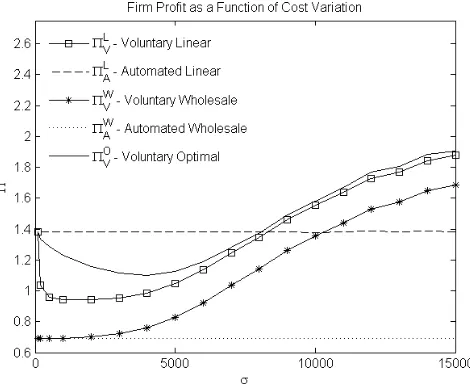
Figure 3: A comparison of contract performance for the firm’s profit
Figure 3 reports the profit performance of each contract studied above for varied values of the standard deviation of C. From Theorem 2, we know that the variance of a symmetric distribution is directly related to the Jensen gap, which affects the profit difference between contract types. Figure 3 demonstrates this result: for sufficiently high variance the voluntary profit curve crosses the automated profit curve for both the full linear and wholesale models. Notice that the two-part tariff linear voluntary profit mirrors the optimal voluntary profit. At its best the two-part tariff achieves 99.9% of the optimal profit, and the two profits are at their closest in the region in which the firm would pick a voluntary contract over an automated contract. As in Cachon and Zhang (2006), we find that the linear contract is a practical substitute for the optimal voluntary contract.
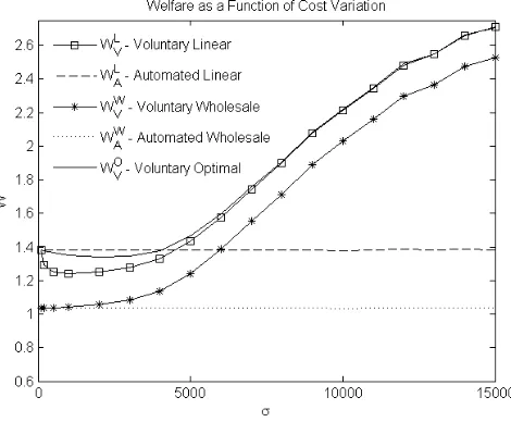
Figure 4: A comparison of contract performance for the social welfare.
Based on our assumptions about the market price of electricity and the curtailment cost of the customer, our model makes several practical recommendations. EnerNOC would be better off introducing a participation fee to extract extra surplus from Four Seasons instead of a no-fixed payment contract. For low levels of cost uncertainty, an automated contract with a two-part tariff is EnerNOC’s most profitable contract choice. For high cost uncertainty, EnerNOC earns a higher profit by offering a voluntary contract. Note that a simple linear voluntary contract is relatively close to optimal in this region.
Furthermore, our experiment suggests that firm and social planner incentives are aligned when the variance of cost is either small or large. When the standard deviation of cost is roughly between [4600,8200]$/M W2, the voluntary contract creates more welfare for the system, but EnerNOC prefers the automated one. In this region, the automated contract allows the firm to extract more surplus, therefore the social planner and the firm incentives are not aligned.
1.8. Conclusion
assume that a curtailing consumer’s load reduction is limited by a stochastic curtailment cost, which is unobserved until the curtailment event. The consumer derives value from the voluntary contract which allows the consumer to observe his curtailment cost before committing to a particular load reduction level. In contrast, the automated contract requires the consumer to commit to a load reduction level without knowledge of his cost. Critically, the firm is punished for suboptimal load delivery through changes in the market price. When deciding between these contracts the firm faces a trade off between the cost of procuring load and the price impact of the load reduction.
Comparing the performance of these two contracts we find that a firm’s and a social plan-ner’s preferences are driven both by market conditions and consumer characteristics. In markets with prices that are highly sensitive to supply, the certainty of the level of cur-tailed load delivered under the automated contract is more valuable to the firm than the reduction in the payments made to consumers under the voluntary contract. This difference in firm profits is also displayed in social welfare. It follows that firms serving as emergency reserves, when the market price curve is at its steepest, should offer automated contracts exclusively. Consumers also determine a firm’s contract choice through their cost profiles. If market price sensitivity is not too high and the curtailment cost distribution has a large Jensen’s gaps, the voluntary contract yields higher firm profit and social welfare. This result distills the contract choice intuition into a single attribute of the consumer’s cost distribution. Furthermore, we show that, for symmetric cost distributions, a firm can use the variance of cost to distinguish between customers that should be offered voluntary or automated contracts: higher variance favors voluntary contracts. As curtailment contracts become more broadly used we hope that these findings will serve as a guide for practitioners to tailor their programs to their market and their customers.
causes the firm to bear price risk, or face uncertain market price caused by the variable curtailment allowed by the voluntary contract. When the market price is sensitive and when consumers derive little value from the flexibility of the voluntary contract, the cost of this price risk outweighs the benefits of flexibility, and the firm prefers the automated contract.
This work has practical implications for regulators in the field of electricity demand re-sponse. We show that, from an environmental perspective, a deregulated market for demand response leads to the ideal contract choice (maximum electricity consumption is avoided). On the other hand, considering the economic surplus of the customer and the curtailment service provider, the firm does not always choose the welfare maximizing contract. A social planner could improve the welfare of the system by encouraging voluntary contracts in some cases in which low cost volatility or high market price sensitivity cause the firm to prefer the automated contract.
CHAPTER 2 : The Role of Surge Pricing on a Service Platform with
Self-Scheduling Capacity
2.1. Introduction
1 The rise of the “sharing economy” has transformed the way firms can deliver service to consumers. The firm no longer must centrally schedule its capacity by assigning workers to shifts. Instead, workers may act as independent service providers who determine their own work schedules, and the firm’s role becomes that of a platform which connects providers to consumers. (See Katz and Krueger (2016) for data on the growth of alternative work arrangements in the United States.) Although the platform has far less control over how many providers work at any one time, providers gain the freedom to “self-schedule” the hours they work, presumably allowing them to better integrate their work with the other activities in their lives (Hall and Krueger (2015b)). To make these new relationships viable, customers must be charged a reasonable fee and be adequately served.
Examples of relatively new platforms that feature self-scheduling capacity include Uber and Lyft for local transportation, and Postmates and Instacart for local delivery. A potential provider for one of these platforms must first make the long-term decision of whether to join the platform or not. This decision has implications for several months or years, and providers join only if they expect to earn more with the platform than with their next best alternative. If a person joins a platform as a provider, then they must make short-term decisions about when and how often to work. These decisions are made on a daily or hourly basis, so the participation decision is relevant over a much shorter time interval than the joining decision. The participation decision is based in part on the wage providers receive per service. It is also based on providers’ expectations of how likely they are to get work, which is a function of the overall level of demand and the number of providers working at that time on the platform. For example, an Uber driver may know that demand is higher on
rainy days but may also know that other drivers are more likely to drive as a consequence. What matters to the provider is the amount of demand relative to the amount of offered capacity at a particular time.
In this paper we focus on the contractual forms a monopoly platform could select to make a viable market with self-scheduling capacity. We study a stylized model with the following features: (i) there exists a large pool of potential providers, (ii) providers join the platform only if their rational expectation of their earnings from participation on the platform exceeds the stochastic opportunity cost of their next best activity, (iii) the platform sets a price for consumers, a wage paid to providers for work completed and regulates the maximum number of providers who join the platform, (iv) the platform cannot directly determine when providers work and, instead, the providers who joined the platform self-schedule their offered capacity, (v) demand is stationary but varies in predictable ways (e.g., more consumers seek transportation on a rainy evening), (vi) if the offered capacity exceeds demand, providers share the available demand equally, but if the offered capacity is less than demand, then demand is randomly rationed (i.e. all consumers are equally likely to receive the scarce service), (vii) the platform’s price and wage can depend on the current level of demand and (viii) provider’s opportunity costs are independent and identically distributed across providers and time.
prices, while the literature on dynamic wages is far less extensive, and there is no work on the interaction between dynamic prices and dynamic wages. Third, capacity decisions are made at two different time scales: providers make a “long run” decision to join the platform or not and then in the “short term” decide whether to participate or not. At the time the participation decision is made, the joining decision (and cost) is sunk.
The platform’s primary goal with the design of its contract is to maximize its profit. Doing so requires a contract that assures providers that join sufficient expected profit. However, the contract must not give providers too much of an incentive to participate, which could lead to an excess of providers, nor too little incentive, which could entice too little participation from providers to satisfy demand.
Although maximizing profit is a clear objective for the platform, it is not the platform’s only concern. A number of controversies have emerged with this new business model. Some people believe providers are not adequately compensated because they are not given bene-fits and rights associated with being employees (Isaac and Singer (2015), Scheiber (2015)). Others worry that customers are unfairly discriminated against as a result of dynamic pric-ing (Kosoff (2015), Stoller (2014)). Consequently, with a view towards potential litigation and regulation, a platform should be concerned with both provider and consumer welfare. In particular, it is important to understand the degree to which there is a tension between maximizing the platform’s profit and the surplus earned by the other relevant stakeholders, the providers and consumers.
the constraint of a fixed commission, i.e., a fixed ratio between the two. The commission contract is used in practice; for example Uber offers its drivers a fixed 80% commission in most markets (Huet (2015)). It has been argued that this constraint may substantially lower the platform’s profit (Economist (2014)). Finally, the platform’s optimal contract dynamically adjusts both prices and wages without the constraint of a fixed commission. A closed form solution for the best version of each of these contracts is unavailable, but we analytically determine how to determine the best form of each contract with a single dimensional search over a bounded space. In addition, we are able to analytically determine conditions under which a commission contract is optimal for the platform. Via numerical analysis over the set of feasible and plausible parameters, we compare profits, consumer surplus and provider surplus across all five contracts. Those results are consistent with the analytical results derived from a special case of the model.
2.2. Literature Review
Our work is primarily connected to three domains in the existing literature: research on capacity and pricing, revenue management models, and recent papers on peer-to-peer plat-forms and self-scheduling capacity. For simplicity and consistency, we refer to the various components in other papers using the terms relevant for our model. For example, the “platform” is the organization responsible for designing the market, “providers” generate capacity, “dynamic prices” are demand-contingent payments from consumers to the plat-form in exchange for service, and “dynamic wages” are demand-contingent payments from the platform to providers.
Several papers study competition among multiple providers and establish that competition can lead to excessive entry (e.g. Mankiw and Whinston (1986)) and a platform should discourage competition to mitigate the losses in system value due to this issue (e.g. Bernstein and Federgruen (2005), Cachon and Lariviere (2005)), but those papers do not consider dynamic wages or prices.
A set of papers considers peak-load pricing, the practice of charging higher prices during peak periods of demand (e.g. Gale and Holmes (1993)). The primary motivation of peak-load pricing is to increase revenue by shifting demand from the peak period to the off-peak period. We do not incorporate this capability into our model. For example, consumers in need of transportation during a rainy evening are unable to postpone their need to a time with better weather.
periods (importantly) have predictably higher demand than others for a given price.
There is a considerable literature on “two-sided markets” in which platforms earn rents by creating a market for buyers and sellers to transact (e.g., a game console maker as the platform between game developers and consumers). These papers tend to focus on which side of the market the platform charges based on the various externalities within the system but they do not consider dynamic demand (e.g., Rochet and Tirole (2006)).
Peer-to-peer service platforms have attracted significant academic interest; e.g. Kabra, Belavina, and Girotra (2015), Hong and Pavlou (2014), Snir and Hitt (2003), Moreno and Terwiesch (2014), and Yoganarasimhan (2013). Those papers investigate how to subsi-dize different market players to accelerate the growth of a peer-to-peer platform, whether consumers have geographic preferences over providers, the influence of platform design on provider quality, and how provider reputation impacts the market. We do not explore those issues: our providers are ex-ante homogeneous and do not build reputations. Fraiberger and Sundararajan (2015) investigate the interaction between ownership and sharing on a peer-to-peer marketplace, a dynamic that is not addressed in our model. Cohen et al. (2016) use Uber transaction data to measure the amount of consumer surplus generated given the im-plementation of surge pricing, but they do not estimate a counterfactual consumer surplus level with other contractual forms.
There is modeling and empirical work on the competition between peer-to-peer service mar-ketplaces and existing markets: Einav, Farronato, and Levin (2015), Zervas, Proserpio, and Byers (2016), Seamans and Zhu (2013), Cramer and Krueger (2016), and Kroft and Pope (2014). We do not directly consider the competition between the platform and incumbents.
are homogeneous, so careful matching does not provide a benefit.
Closest to our work are papers on self-scheduling capacity. Ibrahim and Arifoglu (2015) considers a model in which the platform chooses the number of providers and providers are either assigned by the platform to work in one of two different periods or they self select which of the two periods they work in. Unlike in our model, the platform can directly control the number of providers in the system. Taylor (2016) and Bai et al. (2016) study queuing systems in which a platform creates a market for service where arrivals of consumers and servers are endogenously determined based on decisions to seek and provide service respectively. Their models do not consider dynamic prices or wages, and the number of potential providers is exogenous (i.e., capacity decisions are made on a single, short-term, time scale). Gurvich, Lariviere, and Moreno (2015) studies a model in which a platform directly chooses the number of available providers, the wage for each provider who chooses to work, and a cap on the number of providers who are allowed to work: given the platform’s prevailing wage, more providers may want to work than the platform wants. They do not include dynamic pricing - in all versions of their model the platform selects a single price. They also do not impose an earnings constraint for providers. Instead, they impose an exogenous minimum wage. In our model providers decide whether to join the platform based on rational expectations of future earnings.
2.3. Model
Figure 5: Timeline of events
providers then decides whether to join the platform or not. We refer to this as the “joining” decision. This period represents the providers’ long-term decision. With a ride-sharing platform such as Uber, period 1 would represent a provider’s decision to sign up for Uber instead of Postmates, for example. The second period represents the short-term decisions to work on the platform or not. We refer to this as the “participation” decision. For example, once on the platform, providers for Uber must decide whether to offer their service during a particular day or even a particular hour. Consequently, the participation decision is relevant over a much shorter time interval than the joining decision. Hence, the provider expects to make many of these short-term decisions. For simplicity, we collapse these decisions into a single period.
In period 1 a provider incurs an opportunity cost,c1,for joining the platform and in period 2 the provider can earn a profit from participation on the platform. Hence a provider joins in period 1 only if the provider expects to earn in period 2 at least c1. All providers share the same opportunity cost, so either all are willing to join or none are. Our model approximates a market with a deep pool of potential providers and a highly elastic supply curve: if expected earnings are less thanc1, then the number of interested providers drops substantially, but if greater thanc1, then there is an ample number of interested providers.
not exist a finitecsuch that G(c) = 1. In section 2.5 we consider a simplified version of the model in which the participation is fixed across all providers.
The demand level is the second type of uncertainty. Demand occurs only in period 2 and it can be either “high” or “low”. For example, for a ride-sharing platform, “high” demand could be a rainy evening on a holiday weekend, whereas “low” demand could be a warm Wednesday evening. The platform and the providers can anticipate in period 1 that demand can be either high or low, but they only learn the actual state of demand at the start of period 2, after their joining decision but before their participation decision. Thus, providers make their joining decision before either uncertainty is resolved, but they make their participation decision after observing both demand and participation cost. Note, while each provider observes their own c2, the platform does not observe each provider’s participation cost, so only demand uncertainty is resolved for the platform.
The platform faces a linear demand curve with an uncertain intercept. To be specific, demand for the platform’s service is Dj = (aj−bpj)+, where pj is the price charged to consumers, b is a constant, and the demand state can either by low or high,aj ∈ {al, ah}, where al < ah. Letfj,j ∈ {l, h} be the probability of statej demand, wherefl+fh = 1. Each participating provider can serve up to a single unit of demand in period 2. The parameterb has no impact on the qualitative results, sob= 1 is assumed throughout.
At the start of period 1 the platform announces the terms of trade for providers joining the platform. The terms consist of (i) an upper bound,N,on the number of providers who can join (e.g. Uber imposes a cap on the total number of drivers that can operate in a city), (ii) a price charged to consumers in each demand state,pj,and (iii) a wage paid in each demand state to each provider for service, wj. We say that the platform uses demand-contingent, or dynamic, prices if pl 6= ph. The platform can also choose a single price no matter the demand state, i.e. pl=ph. The same applies for wages.
the capacity of participating providers. In that case demand is randomly rationed: some demand is not served while all participating providers serve one unit of demand. Alter-natively, it is possible that capacity exceeds demand. In that case capacity is rationed: participating providers utilizes only a portion of their capacity. To be specific, let φj be a provider’s utilization in demand stateaj, where φj is the fraction of capacity offered by the participating providers used to serve demand. When demand is rationed, φj = 1, whereas when capacity is rationed, φj <1.
A participating provider earns revenueφjwj in period 2. All providers (who joined in period 1) with participation costφjwj or lower choose to participate, while providers unfortunate to have high participation costs choose not to participate. We require that providers make maximizing decisions based on rational expectation regarding their earnings. (See Farber (2015) and Chen and Sheldon (2015) for evidence that taxi drivers and Uber providers respectively make decisions based on rational expectations to maximize their return.) Thus, assumingN providers join the platform in period 1, in equilibrium
φj =
1 N G(wj)≤aj−pj aj−pj
N G(φjwj) aj −pj ≤N G(wj)
Note that in the second case with capacity rationing, i.e. aj −pj ≤ N G(wj), a recursive relationship determines the equilibrium utilization. This equilibrium utilization exists and is unique.
Let πj be a provider’s expected profit conditional on joining for a given demand state aj, wagewj, and price pj:
πj = (wjφj−Ec2[c2|c2 ≤wjφj])G(wjφj) =
Z wjφj
0
Let Π be a provider’s expected profit from joining the platform:
Π(p, w, N) = X j∈{l,h}
Z wjφj
0
G(c)dc
fj
If c1 ≤ Π(p, w, N), then all potential providers attempt to join the platform, but the platform’s imposed cap of N limits the number that actually join to the N. However, if Π(p, w, N)≤c1, then no providers join. Hence, for the platform to function, it must offer terms such that c1 ≤Π(p, w, N). Throughout we assume that such terms are offered and henceN providers join the platform.
The platform’s objective is to choose price, wage, and recruitment to maximize its expected profit subject to the (already mentioned) constraint that providers are willing to join the platform:
max
w,p,N U(p, w, N) =
X
j∈{l,h}
(pj−wj)φjN G(φjwj)fj
s.t. c1 ≤Π(p, w, N)
It is helpful for our analysis to implicitly define four parameters, w0, w00, ¯φl, and c1:
Rw0
0 G(c)dc=c1;
Rw00
0 G(c)dcfh =c1;
Rφ¯lw
0 G(c)dcfl+
Rw
0 G(c)dcfh=c1; c¯1 =
P
j∈{l,h}
Raj
0 G(c)dcfj
The first,w0, is the smallest wage that induces providers to join when they can assume that they are assured to be paid w0 in either demand state in equilibrium. The second, w00, is similar to w0, except this is the lowest wage that induces providers to join when they are assured to receivew00payment in the high demand state and no payment in the low demand state. (Ifal≤p,then there are no customers to serve in the low demand state.) The third,
¯
system (i.e., ifc1 < c1 then a provider wouldn’t join the platform even if she were the only provider on the platform and the platform allowed her to keep all of the possible profit). Asc1 < c1 means this market cannot function, we assumec1 < c1 throughout.
Beside its own profit, the platform may have an interest in consumer and provider sur-plus, especially if the platform’s practices are potentially controversial, thereby motivating negative publicity, lawsuits, or government regulation. We measure consumer surplus un-der a linear stochastic demand in a similar fashion to Cohen, Lobel, and Perakis (2015):
S =P
j∈{l,h}0.5 min((aj −pj)2,(aj−pj)N G(φjwj))f(aj). Consumer surplus decreases in the prices charged and increases in the number of consumers served. The latter depends on the number of providers that join the platform, N, and the fraction of those recruited providers that decide to participate. Provider surplus increases in the number of recruited providers and in those providers’ expected earnings. If each provider earns exactlyc1 con-ditional on joining (as is shown in each of the contracts we consider), then total provider surplus isc1N.
2.4. Contract Design
We focus on five contract designs that vary by the amount of flexibility given to the platform to adjust its prices and wages in response to observed demand in period 2. A closed form solution for the platform’s best version of each contract is unavailable, but the following five theorems indicate that the platform’s best contract within each design can be found via a single dimensional search over a bounded interval (even though each contract involves up to five decisions: a price and wage for each demand state and the number of providers to allow on the platform). Proofs are available in the appendix.
2.4.1. Fixed Contract
inefficien-cies: demand rationing and capacity rationing. With demand rationing, the offered wage is too low to induce enough providers to participate relative to realized demand, leaving some customers without service. With capacity rationing, the offered wage is too high because too many providers participate relative to realized demand. For a given contract, it is pos-sible that demand is rationed in the high demand state and capacity is rationed in the low demand state, as is illustrated in Figure 6. In the low demand state, N G(φlw) providers participate, which exceeds demand,Dl=al−p. In the high demand state,N G(w) providers participate, all are allocated a customer, butDh−N G(w) customers do not receive service, even though the number of providers on the platform, N, may be adequate to serve all demand.
Figure 6: An example of demand and capacity rationing with a fixed contract.
The fixed contract may not be able to earn a positive profit (given c1 < c1), but if it does so, then Theorem 6 describes the best fixed contract for the platform, which can be divided into two types: (i) the platform serves both demand states, or (ii) the platform only serves high demand. There are two extreme versions of serving demand in both states. In the first, which we refer to as thepoor service version, capacity matches low demand, meaning that there is no capacity rationing and providers are fully utilized in all states. However, while all customers are served in the low demand state, in the high demand state ah−al of demand is lost. In the second version, which we refer to as the poor utilization version, capacity matches high demand. Customers are fully served in either state, but in the low demand state too many providers participate, chasing too little demand, leading to capacity rationing.
Theorem 6. Conditional on earning a positive profit, the best fixed contract has one of the
1. The platform serves both demand states. In particular, w∈[w0,min(al, w00)],
p= max (al+w)/2, G(w)al−φ¯lG( ¯φlw)ah
/ G(w)−φ¯lG( ¯φlw)
there is demand rationing only in the high state ( i.e. N = (al−p)/(φlG(φlw))), there is capacity rationing only in the low state (i.e. φl= ¯φl≤1 and φh = 1), and each provider’s joining constraint is binding, i.e. c1 = Π(p, w, N).
2. The platform serves only high demand. In particular, w = min{w00, ah}, al < p = (ah+w)/2, N = (ah−p)/G(w), and participating providers are fully utilized, i.e. φh= 1.
2.4.2. Dynamic Wage Contract
Theorem 7. Conditional on earning a positive profit, the best dynamic wage contract has
one of the following two characteristics:
1. The platform serves both demand states. In particular,
c1=
Z wl
0
G(c)dcfl+
Z wh
0
G(c)dcfh
p= max
ahG(wl)−alG(wh)
G(wl)−G(wh)
,min
al,
al 2 +
fhG(wh)wh+flG(wl)wl 2(G(wh)fh+G(wl)fl)
there is demand rationing only in the high state ( i.e. N = (al−p)/G(wl)), there is no capacity rationing, i.e. φl =φh = 1, and each provider’s joining constraint is binding, i.e.
c1 = Π(p, w, N).
2. The platform serves only high demand. In particular, wh = min{w00, ah}, p = (ah+
wh)/wh, N = (ah−p)/G(wh), and participating providers are fully utilized, i.e. φh= 1.
2.4.3. Dynamic Price Contract