Globalization and Wage Polarization
∗
Guido Cozzi
†Giammario Impullitti
‡(University of St. Gallen)
(University of Nottingham)
July 18 2015
Abstract
In the 1980s and 1990s, the US labour market experiences a remarkable polarization
along with fast technological catch-up, as Europe and Japan improve their global
inno-vation performance. Is foreign technological convergence an important source of wage
polarization? To answer this question, we build a multi-country Schumpeterian growth
model with heterogeneous workers, endogenous skill formation and occupational choice.
We show that convergence produces polarization through business stealing and increasing
competition in global innovation races. Quantitative analysis shows that these channels
can be important sources of US polarization. Moreover, the model delivers predictions on
the US wealth-income ratio consistent with empirical evidence.
∗We thank the Editor, Philippe Aghion, and two anonymous referees for their comments. We would also like to thank Ufuk Akcigit, Tiago Cavalcanti, David Hemous and seminar
par-ticipants at the Bank of Portugal, Cambridge, Durham, EUI Florence, IAE Barcelona, IIES
Stocklhom, Konstanz, NBER SI, SED Warsaw, Rome Sapienza and Uppsala. A previous
ver-sion of the paper circulated under the title “Globalization, Wage Polarization, and the Unstable
Great Ratio.”
†School of Economics and Political Science, University of St. Gallen. Email: [email protected].
‡School of Economics, University of Nottingham. Email:
JEL Classification: F16, J31, O33
Keywords: wage polarization, heterogeneous workers, wealth-income ratio, en-dogenous technical change, international technology competition, personal service sector.
1
Introduction
The US labour market has experienced a radical polarization of employment and wages in the
last decades. In the 1980s and 1990s, both wages and employment shares at the tails of the
skill distribution have grown steadily. Workers in the middle of the distribution instead have
faced stagnant wages and shrinking employment share (Acemoglu and Autor, 2011). Recent
empirical work has shown that also the wealth to income ratio has been increasing steadily since
the mid-1970s in the US (Piketty and Zucman, 2014). Here, we make an explorative attempt
to assess the role of globalization, in the form of fiercer foreign technological competition, in
shaping these important developments of the US economy.
In the years of expanding labour market polarization, the US economy became increasingly
globalized. The massive reduction in trade barriers and the diffusion of technologies across
countries’ borders allowed foreign firms, mostly from Japan and Europe, to challenge US
tech-nological leadership. The geography of techtech-nological leadership, measured as countries’ share
of innovation inputs and outputs, shows remarkable changes between the mid-1970s and the
late 1980s. As the distribution of leadership moved from drastically skewed toward the US, to
a more equal global playing field, clear convergence patterns can be observed in the share of
patents, patent citations and R&D spending. The share of foreign patents in the US Patent
Office, was about one third in 1977 and grew to about one half ten years later. The US share
of global industrial R&D declined from about 50 percent in 1979 to 39 percent in 1995. Most
of this technological catching-up was due to a massive acceleration in Japanese innovation
ac-tivity, although some European countries, such as Germany and France, played a major role in
Did the acceleration of foreign technological competition in the 1980s contribute to the
polarization of the US labour market? To answer this question we construct a quality
lad-der growth model (Aghion and Howitt, 1992, and Grossman and Helpman, 1991) with two
asymmetric countries and heterogeneous workers. Firms compete for global market leadership
investing in quality-improving innovation. Schumpeterian competition for innovation allows
successful innovators to replace incumbents. The asymmetry between countries is represented
by a technology gap in innovation: firms in the leading country have a better innovation
tech-nology in all sectors of the economy. There are three occupations: innovation, production, and
services: innovation workers are employed in the production of new ideas to improve the quality
of the goods. Blue collar, production workers, are employed in the manufacturing of goods.
Service sector workers provide personal services that allow their employer to save working time.
Workers have heterogeneous ability and can acquire working skills through education.
Educa-tional attainment allows workers to become skilled and work in innovation activities. Workers
who do not acquire education can work as production workers or in service occupations.
In equilibrium, the following allocation of abilities to occupations is obtained: workers with
high innate ability become skilled and hire service sector workers, those with intermediate ability
work in production occupations and finally, those at the bottom of the ability distribution work
in personal service occupations. Reductions in the technology gap has the following effects on
the leading economy: First, as foreign firms start innovating more efficiently, they obtain quality
leadership in more sectors, thereby stealing market shares from firms in the leading country
and reducing the demand of production workers. This business-stealing effect reduces wages
of production workers in the leading economy. Second, the reduction in the technology gap
makes it harder for domestic firms to innovate in the global economy, thus pushing them to
devote more labour resources to innovation. This global competition effect triggers an increase
in the demand for skilled workers. Via these two channels, increasing foreign competition
generates more polarization in the leading economy’s labour market: the wage of skilled workers
relative to that of production workers increases, thereby raising inequality at the top of the skill
thus reducing inequality at the bottom of the distribution. The increase in the demand and
wages of service sector workers is a by-product of rising inequality at the top of the distribution.
As skilled labour time becomes more valuable, skilled workers demand more personal services
in order to free time to devote to their highly remunerative job.
Another key prediction of our model is the positive link between foreign technological
com-petition, innovation, and the wealth-income ratio. The business-stealing and the global
compe-tition effect of foreign technological catching up increase the value of innovation in the global
economy. In our Schumpeterian economy, the value of innovation is determined by the value
of the leading firm in each product line, and aggregate wealth consists in the sum of the
mar-ket values of all leading firms. Hence, our model establishes a natural connection between
international competition, innovation and the dynamics of the wealth-income ratio.
In an extended version of the model, we allow for a more general technology where skilled and
unskilled workers are employed in production and innovation with different factor intensities,
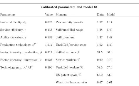
we introduce iceberg trade costs, and we specify the workers’ ability distribution. We then
calibrate this generalized model and use it to explore the link between the technology gap,
labour market polarization and the wealth-income ratio quantitatively. In our two-country
world, the US is the leading economy and the rest of the world represents the foreign country.
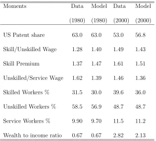
The technology gap between countries is calibrated to reproduce the distribution of patents in
the US Patent Office. A closure of the innovation technology gap reproduces a sizable part of
the convergence in US and foreign patent shares shown in the data between 1980 and 2000,
along with a non-negligible share of wage and jobs polarization: our model can replicate about
10% of the increase in inequality at the top of the distribution, 16% of the increase in the skill
premium and about 18% of the decrease in inequality at the bottom observed between 1980
and 2000. Finally, the decline in the technology gap generates a striking increase in the US
wealth-income ratio, reproducing about two thirds of the change documented by Piketty and
Zucman (2014).
The recent empirical evidence on labour market polarization in the US has triggered a
simple “task-based” model with capital-skill complementarity formalizing the so-called
”rou-tinization” hypothesis. This hypothesis posits that technological change complements skilled
tasks, replaces routine tasks, and is neutral to service occupations. Hence technology affects
the wage structure through a postulated factor bias. We propose a complementary approach
according to which polarization is driven by the factor intensity of innovation rather than the
factor bias of technological progress. Moreover, Autor and Dorn treat technological progress
and the supply of skills as exogenous.1 We complement their analysis by endogenizing both
technological change and skill formation, as well as by exploring the key role of globalization.
In our economy, the increase in the demand and wages of service sector workers relative to
other unskilled tasks comes from a general equilibrium market mechanism: foreign competition
raises inequality at the top of the distribution, thereby inducing skilled workers to demand
more personal services and devote more time to their highly paid jobs. This mechanism finds
direct empirical support in Mazzolari and Ragusa (2013) who, using US city-level data, show
that the increase in the top wages bill can explain about one-third of the growth of employment
of non-college workers in low-skill personal services in the 1990s.
Finally, our paper is also related to the literature on globalization and wage inequality. A
large body of work has studied the effects of trade liberalization on wage inequality across
work-ers with different skills when technology is constant (e.g. Epifani and Gancia, 2008, Burstein
and Vogel, 2010), or when technology is endogenous and interacts with trade in shaping the
wage structure (e.g. Dinopoulos and Segerstrom, 1999, and Acemoglu, 2003). We depart from
this literature along two main lines: first, while existing papers focus on economies with two
skills and explain the evolution of the skilled-unskilled wage gap, the skill premium, we work
in environments with a continuum of skills allocated to different occupations which allows us
to study inequality in several parts of the wage distribution. Second, we move from a widely
studied dimension of globalization, trade liberalization, to the less explored channel of
cross-1Hemous and Olsen (2014) embed the routinization hypothesis into a fully-fledged dynamic
model of directed technical change and show that technological progress can generate phases
country technological catch up. A small emerging literature has started to analyze the effects
of foreign technological catching up on growth and welfare (e.g. Eaton and Kortum, 2007, Hsie
and Ossa, 2011, Impullitti, 2010, Akcigit, Ates, and Impullitti, 2014). Our paper contributes
to this line of research studying the effects of foreign catching up on the structure of wages,
employment, and on the evolution of the wealth to income ratio.2
2
Stylized facts
In this section, we discuss some key facts providing the motivation for the paper as well as
empirical support for the quantitative analysis.
Wage polarization. Since the early 1980s, the US has shown a remarkable increase in labor
market polarization. Autor and Dorn (2013) document a non-monotonic change in employment
and wages along the skill distribution. Working with Census IPUMS and American Community
Survey data, they rank 318 occupations in all US nonfarm employment by skill level using the
average wages of workers in each occupation. Their results show that employment changes in
the period 1980-2005 have an inverted U-shaped pattern. Employment in the middle of the
skill distribution declines substantially, while the tails show a steady and somewhat puzzling
increase. Digging deeper into the occupational structure of these changes they document that
most of the increase in employment and wages in the lower tail can be attributed to one group of
occupations that they name service occupations. These are low-education occupations
involv-ing carinvolv-ing, assistinvolv-ing and entertaininvolv-ing other people, such as, cleaners, janitors, security guards,
food service workers, gardeners, home health aides, hairdressers, beauticians, and recreation
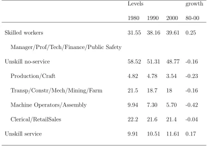
occupations. Table 1 below shows the employment dynamics for three groups of occupations.
Skilled workers include the occupations at the top of the skill distribution. Unskilled workers
outside service occupations comprises a low-educated occupational group including production
and crafts jobs, operative and assembly occupations, transportation, construction, mechanical,
2Impullitti (2015), analyses the effects of foreign competition on the skill premium and on
mining, clerical and retails sales jobs. The third group includes the service occupations
de-scribed above. The data show a strong increase in the employment share of skilled workers,
which grew by 25% between 1980 and 2000. Similarly, the employment share of service
occu-pations increased by about 17% in the 1980-2000 period. On the other hand, the employment
Table 1: Employment Share by Major Occupation Groups: 1980-2000
Levels growth
1980 1990 2000 80-00
Skilled workers 31.55 38.16 39.61 0.25
Manager/Prof/Tech/Finance/Public Safety
Unskill no-service 58.52 51.31 48.77 -0.16
Production/Craft 4.82 4.78 3.54 -0.23
Transp/Constr/Mech/Mining/Farm 21.5 18.7 18 -0.16
Machine Operators/Assembly 9.94 7.30 5.70 -0.42
Clerical/RetailSales 22.2 21.6 21.4 -0.04
Unskill service 9.91 10.51 11.61 0.17
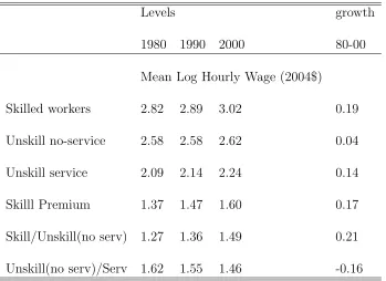
Table 2: Mean Real Hourly Wages by Major Occupation Groups: 1980-2000
Levels growth
1980 1990 2000 80-00
Mean Log Hourly Wage (2004$)
Skilled workers 2.82 2.89 3.02 0.19
Unskill no-service 2.58 2.58 2.62 0.04
Unskill service 2.09 2.14 2.24 0.14
Skilll Premium 1.37 1.47 1.60 0.17
Skill/Unskill(no serv) 1.27 1.36 1.49 0.21
Unskill(no serv)/Serv 1.62 1.55 1.46 -0.16
Table 2 shows the levels and changes in wages for the three groups of occupations in the
same period. We can see a substantial increase in wages of skilled workers and a smaller but
negligible increase in service occupations’ wages. The wages of unskilled workers in
non-service occupations instead exhibit virtually no change. Focusing on the relative changes across
these groups, we can look at the dynamics of the gap between the top and the middle of the
distribution and that between the middle and the bottom. The first gap is represented by
the ratio of skilled over unskilled (non-service) wages, which shows a 21% increase up to 2000.
The second gap is the ratio between the wages of unskilled workers outside of personal service
occupations and those of service workers. This ratio declines by 16 percentage points up to
2000. We also compute a more standard measure of inequality, the skill premium, defined as
the average wage of skilled workers over of the average wage of all unskilled workers, including
service sectors workers.3 In line with inequality at the top of the distribution, the skill premium
shows a remarkable increase after 1980.
The wealth to income ratio. Piketty and Zucman (2014) report that the wealth to income
ratio in the US rose from slightly above 350% in 1980 to 450% in 2000. The wealth of a nation
is defined as the sum of domestic capital and net foreign assets. In the US, the foreign asset
position in those years is negligible, hence the wealth to income ratio and domestic capital to
income ratio coincide. For this reason, they use the terms wealth-income and capital-income
ratio interchangeably. Capital in the data is the sum of agricultural land, housing, the value
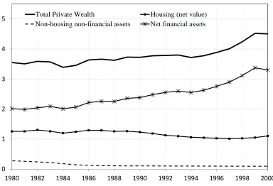
of financial assets net of liabilities and the value of net non-financial assets. Figure 2 shows
the evolution of private wealth and its components in the period we are analyzing. As we can
see, financial wealth is the driving force of the increasing wealth to income ratio, while housing
wealth (net of mortgages) and non-financial assets, which include tangible capital, are fairly
constant. 4
3The average unskilled wage is obtained using the employment shares of the unskilled (no
service) and service occupation workers as weights.
4Non financial assets include produced tangible capital and non-produced tangible capital.
fixed assets: buildings and structures, machinery and equipment, cultivated biological resources,
Figure 1: Composition of Private Wealth, 1980-00, % National Income
0 1 2 3 4 5
1980 1982 1984 1986 1988 1990 1992 1994 1996 1998 2000
Total Private Wealth Housing (net value) Non-housing non-financial assets Net financial assets
About two thirds of financial assets are accounted for by corporate wealth. In Figure 2,
we report the two measures of corporate wealth constructed by Piketty and Zucman (2014).
The first measure is the equity value, which is the market value of the firm, and the second is
the net worth, which is the “book value” of the firm which comes from a perpetual inventory
method-based estimates of tangible assets. The difference between the two measures is the
Figure 2: Corporate Wealth, 1980-00, % National Income
0 0.5 1 1.5 2 2.5 3
1980 1982 1984 1986 1988 1990 1992 1994 1996 1998 2000
Net worth Equity Value Equity/Net Worth (Tobin Q)
Both measures of corporate wealth exhibit a striking increase in the period of interest. The
book value rises from 150% of income in 1980 to 220% in 2000, while the equity value from
67% in 1980 skyrockets to 280% in 2000.
International technological competition. During this period of increasing wage
polariza-tion and fast growing wealth-income ratio, the US experienced increasing foreign technological
competition. The data show a global convergence pattern in several measures of innovation
performance. The US, the undisputed technological leader in the post-World War II period,
was progressively challenged by Japan and European countries in the late 1970s and 1980s.
Figure 3, shows the stark convergence in patent shares in the US Patent office; in 1977 about
two thirds of patents came from American firms, while ten years later only one half of patents
had US origins. Most of the convergence takes place in the 1970s and 1980s, while the following
Figure 3: Share of US and Foreign Patents in US Patent Office
0.3 0.35 0.4 0.45 0.5 0.55 0.6 0.65 0.7
1975 1980 1985 1990 1995 2000 2005
Foreign share US share
This convergence in patenting activity did not happen because of a slowdown in US
patent-ing but it is due to a stark acceleration in foreign patents. The number of foreign patents grew
by about 60% between 1977 and 1988, while US patents did not show any sensible change in
those years. This increase is mainly driven by Japan, whose share rose from 9% in 1977 to
about 20% in 1988. Along these lines, Akcigit, Ates, and Impullitti (2014) show that a similar
trend can be seen in patent citations. Disaggregating at the level of technology classes, they
document a convergence trend in global patenting also at the micro/sectorial level. Together
with convergence in innovation output (patents), recent research has also highlighted similar
patterns for global innovation inputs. Impullitti (2010) documents a strong convergence in
private R&D spending between the US and a group of fast growing advanced economies in the
1970s and 1980s.
3
The model
In this section, we present the baseline model and use it to analyze the interaction between
globalization, innovation and the occupation and wage structure.
3.1
Households
Consumption. The economy is populated by two regions with the same population and
preferences. In both regions, households are heterogeneous in their abilities to acquire skills.
At birth, members draw their ability θ ∈ [0,1] from a distribution Γ(θ). Households have
identical preferences for a continuum of consumption goods ω ∈ [0,1], and each is endowed
with a unit of labour or study time whose supply generates no disutility. Household of type θ
is modelled as dynastic family that maximizes intertemporal utility
U = Z ∞
0
N(0)e−(ρ−n)tlnuθ(t)dt, (1)
where population is specified according to N(t) = N(0)ent, with initial population N(0)
ρ > n. The utility per person is given by
uθ(t)≡ Z 1 0
jmax(ω,t)
X
j=0
λjdθ(j, ω, t)
η−1
η dω η η−1
, (2)
where dθ(j, ω, t) is the per member quantity of good ω ∈ [0,1] of quality j ∈ {0,1,2, ...}
purchased by a household of ability θ at timet ≥0. A new vintage of good ω yields a quality
λ times that of the previous vintage, with λ > 1. Different versions of the same good ω
are regarded by consumers as perfect substitutes after adjusting for their quality ratios, and
jmax(ω, t) denotes the maximum quality in which the good ω is available at time t. Parameter
η∈[1,∞) is the elasticity of substitution across varieties, which allows for gross substitutability
across varieties.
At each point in time, households choose the quantity purchased of each gooddθ(j, ω, t) in
or-der to maximize (2) subject to the per period expenditure constraintR1
0 dθ(j, ω, t)p(j, ω, t)dω=
cθ(t), where cθ(t) is planned time t consumption expenditure. Notice that the household will
be purchasing in each line only the product with the lowest price per unit of quality. Hence,
household’s demand for each product is:
dθ(j, ω, t) =cθ(t)
q(ω, t)P(t)η−1
p(j, ω, t)η , (3)
whereq(ω, t) =λ(η−1)jmax(ω,t)
represents the quality of goodω andP(t) is a general price index,
defined as:
P(t) = Z 1
0
q(ω, t)p(jmax(ω, t), ω, t)1−ηdω
1−1η .
Notice that the quality of the demanded version of a variety, q(ω, t), positively affects its
quantity, while negatively affecting the overall price index. Given the optimal allocation of
expenditures across different product lines at a given moment t in (3), households choose
the intertemporal allocation of consumption maximizing (1) with respect to the intertemporal
yields
·
cθ(t)
cθ(t)
=r(t)−ρ, (4)
the standard Euler equation for consumption.
Supply of skills and personal services. Individuals are finitely-lived members of
infinitely-lived households, being continuously born at rate βn and dying at rate δ, with βn−
δ = n > 0; V > 0 denotes the exogenous duration of their life5. They choose to acquire
education and become skilled, if at all, at the beginning of their lives;and for the duration of
their schooling period, denoted TH < V, the individual cannot work. We assume agents have
heterogeneous innate abilities drawn from a cumulative distribution function Γ(θ).
In country K = D (domestic), F (foreign) an individual with ability θ decides to acquire
education if the expected wage income is larger than that of working as unskilled, that is:
Z t+V
t
e−Rtsr(τ)dτθwK
L(s)ds≤ Z t+V
t+TH
e−Rtsr(τ)dτmax (θ−γ
H,0)wKH(s)ds, (5)
where wLK and wkH are the wage per unit of abilities of the unskilled and skilled workers,
respectively. Parameter 0 < γH < 1 establishes a threshold ability requirement so that an
agent with ability θ > γH is able to accumulate θ−γH units of skills after schooling, while a
person with ability below γH gains no skills from education. Parameter γH can be interpreted
as a fixed cost of education in terms of the skilled wage. We will here focus on steady-state
analysis, in which all variables grow at constant rate andwL,wH, andcθ are all constant. From
the Euler equation (4) we obtain r(t) = ρ at all dates. Equation (5) yields the cutoff ability
level θ0K above which agents acquire education:
wK H
wK L
=σ1
θK
0
θK
0 −γH
, (6)
with σ1 ≡
eρV −1
/ eρ(V−TH)−1 > 1. Notice that, since 0 < γ
H < 1, we have that an
5It is easy to show that the above parameters cannot be chosen independently, but that
they must satisfy δ =n/(enV −1) and β =nenV/ enV −1
in order for the number of births
increase in the relative skilled wagewK
H/wKL reduces the ability cutoff to acquire education θ0K.
Each unskilled individual can work either in production occupations or as a personal
ser-vice worker. Personal serser-vices allow people to spend less time on house chores, baby-sitting,
transportation, and other activities, which would otherwise detract time from other kinds of
activities, such as production and innovation occupations. Since in this model individuals do
not have a desire for leisure, we can assume that each hour saved thanks to service workers
will be used to work more. We will also posit that there is an upper bound, normalized to 1,
of the extra work made possible by personal services.6 Moreover, each unit time of personal
service provides its employer, who must be a different person, 1− extra time for work, with
0 < < 1. This implies that in equilibrium, unskilled workers of same or lower ability levels
will not demand services, because it would cost wKL to obtain an extra labour time which pays
wK
L (1−).
A high skilled worker of generic abilityθ finds it profitable to buy personal services from an
unskilled worker of abilityθ0, if at the cost of θ0wK
L they can obtain an additional wage income
wK
H(1−)θ ≥ θ 0wK
L. The lowest possible θ at which hiring a personal service is worthwhile in country K, denoted θK
HS, and the higher possibleθ
0 supplied by the unskilled, denoted θK LS, must equalize the service cost and employer’s economic benefit, that is:
θKLSwKL =wKH (1−)
θKHS−γH
. (7)
The mass of service workers must be equal to the mass of skilled workers employing them,
Γ(θKLS) = 1−Γ(θKHS). (8)
Plugging equation (8) into (7) and solving forθK LS gives
θKLS(θHSK )≡Γ−1 1−Γ(θHSK ) = w
K H
wK L
(1−)
θKHS−γH
, (9)
which since Γ−1(.) is monotonically increasing, givesθK
HS as a decreasing function of the relative skilled wage, and thereforeθK
LS as an increasing function of the relative skilled wage. Intuitively, a higher relative remuneration of skilled occupations increases the demand for service
occupa-tions. Hence, invoking (6), we can write, dθHSK /dθ0K >0 and dθKLS/dθ0K <0.
The fraction of the population opting out of education determines the per capita supply
of unskilled labour LK ≡ e
θK
LΓ(θ0K), where θeKL = RθK0
0 θdΓ(θ)/Γ(θ
K
0 ) is the average ability of a
generic unskilled worker. Notice that dLK/dθK
0 =θ0K > 0, the supply of unskilled workers, is
increasing in θK
0 . Intuitively, a higher relative skilled wage reduces the cutoff ability to acquire
education θK
0 , thereby reducing the share of unskilled workers. A fraction 1−Γ(θK0 ) of the
population decides to attain education and the skilled workforce is represented by the subset
of these agents that as of date thave completed their schooling period, that is individuals born
between t−V and t−Tr. The per capita supply of skilled labour in efficiency units at time t
is then
HK =θeKH
1−Γ(θK0 ) Z t−T r
t−V
βnN(0)ensds=eθKH
1−Γ(θK0 )φ, (10)
with 0< φ≡ en(V−Tr)−1/ enV −1<1 and
e
θKH = (2−) Z 1
θK HS
(θ−γH)
dΓ(θ) 1−Γ(θK
0 )
+ Z θKHS
θK
0
(θ−γH)
dΓ(θ) 1−Γ(θK
0 )
(11)
is the average ability of educated workers, which takes into account that above the cutoff θK HS
workers get and extra 1−working time from hiring service workers. Using (11) we derive
dHK/dθK0 =−
(1−)dθ K HS dθK 0 + 1
(θ0K−γH)Γ0(θ0K)φ <0,
hence the supply of skills is decreasing in θK
0 .
3.2
Production
In each country, firms can hire unskilled workers to produce consumption good,ω ∈[0,1],under
unskilled wage rate iswK
L and we setwLF = 1, so that the unskilled foreign wage is the numeraire of this economy. Assuming instantaneous price competition, Bertrand equilibrium implies that
in each industry only the product with the highest quality is produced. Quality leaders in each
sector are challenged by followers that employ skilled workers to discover the next top-quality
product. In this model, as typical of quality ladder frameworks, a patent expires as soon as
the next top-quality product is invented. Successful innovation yields global market leadership,
which is protected by a perfectly enforceable patent law.
We assume that the technologies to produce goods one quality ladder below the top are
obsolete and diffuse freely. This assumption allows foreign successful innovators to become
global market leaders.7 We allow for international trade in goods, but we do not consider
multinational companies in this model. In addition, while allowing for perfect patent protection,
we rule out an international market for patent royalties. Therefore, in our model, only domestic
firms can produce and export the goods patented in the country. Finally, we do not consider
international trade in assets.
As will become clearer in the next sections, as a consequence of the technology gap between
the two countries, country D has global market leadership in a wider range of sectors, which
drives up the demand for its manufacturing labour. For this reason, in all our equilibria the
unskilled wage in countryDwill be higher than that of countryF, that iswLD > wLF. Since both
domestic and foreign followers operate with the same technology, and foreign unskilled labour
is cheaper, domestic followers are not an effective competitive threat. Moreover, we assume
that the quality jump λ is not high enough that each top-quality producer firm can maximize
7Without this assumption if a leader experiences successive innovations, followers will be
pushed out of the market permanently. The assumption of immediate diffusion of the old
production technology is discussed in Glass (1997) and widely used both in North-North models
of trade and growth (e.g. Dinopoulos and Segerstrom, 1999), and in North-South models (Glass,
profits unconstrained in both markets8. Thus the price of a top-quality good in a sector ω is
pK(jmax(ω, t), ω, t) = λwLF(t) =λ >1. (12)
Notice that this implies that wD
L ≤ λwFL, because otherwise country D firms would lose all markets and unskilled jobs9. This ”narrow gap” case (Grossman and Helpman, 1991) allows
for equilibrium product-cycle trade (Vernon, 1966) with global market leadership shifting from
domestic to foreign firms as the latter innovate and viceversa. Although the foreign region has
a cost advantage in production, equilibrium guarantees that the wage gap is not so large that
a foreign follower can price a domestic leader out of the market without innovating.
From demand (3), we conclude that the demand for each product ω is
N(t)(cD(t) +cF(t))q(ω, t)P(t) η−1
p(j, ω, t)η =d(ω, t) , (13)
where cK(t) = R1
0 c
K
θ (t)dθ is average per capita expenditure. Notice that under the pricing condition (12) the price index becomes, P(t)η−1 =λη−1
/Q(t), whereQ(t) = R01q(ω, t)dω is the
average quality in the economy. Therefore, using (13) and dropping time indexes for notational
simplicity, we can write:
d(ω) = N(c
D +cF)q(ω)
λQ , forω ∈[0,1]. (14)
Since supply and demand of goods are equal in equilibrium, the stream of monopoly profits
accruing to domestic quality leaders is πD
n(ω) =N(cD +cF)q(ω) λ−wLD
/λQ, and the profit
of the foreign leader is πF(ω) = N(cD +cF)q(ω) (λ−1)/λQ.
8Cases in which this does not hold can be easily handled, with no qualitative change in the
results.
9This includes those in the service sector, because innovation would stop - due to lack of
3.3
Global innovation races and the value of a firm
In each industry, firms employ skilled workers to discover the next top-quality version of their
products. The arrival rate of innovation in industry ω at timet is I(ω, t), which is the sum of
the Poisson arrival rate of innovation produced by all firms targeting productω. The innovation
technology available to a firm i in region K for innovation in sector ω is
IiK(ω, t) =
AKhKi (ω, t)HXK((ω,tω,t)) −α
X(ω, t) , (15)
where hK
i (ω, t) is labor input in innovation by firm i, in industry ω, and X(ω, t)>0 measures the degree of complexity of innovation, α is a positive congestion parameter, and HK(ω, t) = P
ih K
i (ω, t) and IK(ω, t) = P
iI K
i (ω, t) are the total skilled labour and the total innovation rates in sectorωrespectively. This technology implies that each firm’s instantaneous probability
of success is a decreasing function of the total domestic labour resources devoted to innovation
in an industry. A possible interpretation of this property is that when firms increase
innova-tion inputs in a sector, the probability of duplicative innovainnova-tion effort also increases, thereby
reducing the probability that any single firm discovers the next vintage of goods. Therefore,
the sector-specific negative externality in innovation technology produces decreasing returns to
innovation at the industry level. Moreover, (15) implies that this negative externality is also
region-specific.10
Notice that equation (15) implies IK(ω, t) = AK HK(ω, t)/X(ω, t)1−α
. The
complex-ity index X(ω, t) is introduced to avoid the counterfactual prediction of the first generation
innovation-driven growth models that the size of a region affects its steady-state growth (Jones,
10There is strong empirical evidence on the nonlinearity of the relationship between innovative
activity of a country (measured using patent data) and its R&D investment. Working with a
large sample of US firm-level data, Hall et al. (1986) find an elasticity of patents to R&D of
0.5. The evidence surveyed in Kortum (1993) suggests point estimates for the patent/R&D
elasticity in the range 0.1 - 0.6. More recently, Blundell et al. (2002) find a long-run elasticity
1995). We eliminate the strong scale effect by assuming
X(ω, t) = q(ω, t)
Q(t)φ1 (16)
with 0< φ1 <1. Therefore, the more advanced the good relative to the average quality the more
difficult a further innovation. Moreover, even for an average quality good (i.e. if there exists an
ω such that q(ω, t) =Q(t)), the higher the average quality itself the more difficult innovation
(in this caseX(ω, t) =Q1−φ1
t ), which incorporates Jones (1995) increasing complexity argument to rule out the strong scale effect. Equation (16) implies that, log-differentiating the difficulty
index between quality jumps in the sector, its evolution obeys ˙X(ω, t)/X(ω, t) =−φ1Q˙(t)/Q(t).
Each innovating firm chooses the labour resources devoted to innovation hK
i in order to maximize its expected discounted profits. Free entry into innovation races drives profits to
zero, yielding
vK(ω, t)
IK(ω, t)
AK
1−−αα AK
X(ω, t) =w K
H(t), (17)
where vK(ω, t) is the value of a firm in sector ω and country K. This condition states that
the cost of one unit of skilled labour employed in innovationwKH must be equal to its benefits,
represented by the marginal product of labor in innovation AK LK(ω, t)/X(ω, t)−α
/X(ω, t)
times the prize for a successful innovationvK(ω, t). Notice that, despite the leaders and followers
having the same production and innovation technology, the free entry condition implies that
we can compute the equilibrium focusing only on the followers’ innovation.11
Efficient financial markets channel savings into innovative firms that issue a security paying
the new monopoly stock market value if they win the race and zero otherwise. Since there is
a continuum of industries, and simultaneous and independent innovation races, consumers can
perfectly diversify away risk: the expected rate of return of a stock issued by a firm is equal to
the riskless rate of return r(t). It is easy to show that this leads to the following stock market
11This is the celebrated Arrow effect (see Cozzi, 2007), introduced by Aghion and Howitt
value of a firm:
vK(ω, t) = π
K(ω, t)
r(t) +I(ω, t)−v·K(ω, t)/vK(ω, t)
, (18)
where I(ω, t) denotes the worldwide Poisson arrival rate of an innovation that will destroy the
monopolist’s profits in industryω. This is the Schumpeterian rate ofcreative destruction, which
implies that the expected value of a patent is decreasing in the total innovation of the industry.
Substituting for the value of the firm from (18) into (17) and using (15) to express the amount
of skilled workers in terms of the innovation rate we obtain the following conditions
πK(ω, t)
r(t) +I(ω, t)−v·K(ω, t)/vK(ω, t)
IK(ω, t)
AK
1−−αα AK
X(ω, t) =w K
H(t), for ω∈[0,1] andK =D, F. (19)
These conditions, together with the Euler equation, summarizes the utility maximizing
house-hold choice of consumption, savings, and education, and the profit maximizing choice of
pro-duction and innovation. Innovation arrival rates determine the evolution of the average quality
of goods in the economy Qt. Finally, in all industries, firms from both regions compete in
in-novation. Hence global innovation in each sector isI(ω, t) =ID(ω, t) +IF(ω, t), whereID(ω, t)
and IF(ω, t) are domestic and foreign innovation.
Assumption 1 (Technology Gap). AD > AF.
We introduce a gap between the two countries in terms of the innovation technology
pa-rameter A. Since goods ω ∈ [0,1] are symmetric (same technologies, both in production
and innovation, and enter the utility function symmetrically), the only source of structural
asymmetry between the two countries is the difference between their innovation productivity.
Since there is no sectorial heterogeneity in this economy, we can write, ID(ω, t) = ID(t) and
IF(ω, t) = IF(t) for all ω. In a steady state, the per industry probabilities of innovation per
unit of time will be constant over time, which allows us to drop time indexes and write ID and
IF. DifferentiatingQ with respect to time, it is straightforward to prove that:
g = Q˙
Q = λ
η−1−1
The growth rate of aggregate quality is proportional to the global arrival rate of innovation.
3.4
Labour markets
The production technology specified above implies that the demand for unskilled workers is
equal to the total production of goods in each national economy plus the total demand for
personal services. The unskilled labour market clearing condition is
Γ(θ0K)−(1−Γ(θHSK )) e
θKM = (c
D+cF)
λ q
K, (21)
where θeKM = RθK0
θK LS
θKdΓ(θ)/ Γ(θK
0 )−Γ(θLSK )
is the average ability of unskilled workers
em-ployed in production. The left-hand side is the supply of unskilled workers in
manufactur-ing in efficiency units. The right-hand side is the demand for unskilled workers. We define
qK =QK/Q, as the share of sectors with country K0s leadership, where QK =R
BKq(ω)dω is the average quality of the sectors in which country K has global leadership (BK is the measure
of these sectors), and qD +qF = 1 by construction.12
The market clearing condition for skilled workers is
e
θKH(1−Γ(θK0 )φ=
IK
AK
1/(1−α)Z 1
0
X(ω)
N dω=
IK
AK
1/(1−α)
x , (22)
where we define x = Q1−φ/N = R1
0 X(ω)dω/N, which is the aggregate difficulty index of
innovation normalized by population. The left-hand side is the domestic supply of skilled
labour (per capita) from (10), and the right-hand side is the domestic demand for skilled
workers obtained after integrating equations (15) and (16).
12At any point in time BD ∪BF = [0,1]; that is, each sector is either monopolized by a
country D firm or by a country F firm. The measure of such sets is qD, respectively qF,
with qD +qF = 1. Notice that each BK changes over time as firms of different countries
alternate their market leadership, but in the steady state its measure is constant. Moreover,
˙
Wage Inequality. Since our main aim is to analyze the link between the technology gap
and wage inequality, we need to specify the measures of inequality we want to focus on. The
education choice and demand for service sector workers partition the worker/ability space as
follows. Skilled workers are those whose abilities lie in θKHS,1, who hire unskilled workers to
perform personal services and therefore have extra time and income, and those, with ability in
[θK
0 , θKHS), who do not hire unskilled workers for performing personal services. The unskilled workers with ability in (θK
LS, θK0 ] work in the manufacturing sector, while those in
0, θK
LS
work
in services. Hence, the average wage of skilled workers is the skilled wage per unit of skills
wD
H times the average skill level of educated workers, ˜wHD =wDHθeDH. Similarly, the average wage of the unskilled workers employed in production and the average wage of the service sector
workers are
˜
wDL =wDLθeMD =wDL Z θ0D
θD LS
θ dΓ(θ)
Γ(θD
0 )−Γ(θDLS)
, ˜wSD =wLDθeDS =wDL Z θDLS
0
θ dΓ(θ)
Γ(θD
0 )−Γ(θLSD )
(23)
respectively. We will mainly focus on two wage gaps: the skilled/unskilled (production) workers
gap and the unskilled (production)/service workers gap,ωH = ˜wHD/w˜DL andωS = ˜wDS/w˜LD, both
depending on the relative wage and on the relative average ability of workers.
4
Steady-State Equilibrium
A balanced growth path for this economy is an equilibrium in which per capita consumption
cK, innovation IK, the share of industries with a domestic leader qD, wages wK
H and wKL, and the ability cutoffs θK
HS and θ0K are constant, while the average quality of goods Q grows at a
constant rate. Since wages and sectorial innovation probabilities are constant in steady state,
the free entry condition (17) and (16) imply that v·K(ω)/vK(ω) = X· (ω)/X(ω) = −φ
1Q/Q˙ ,
for K = D, F and for all ω ∈ [0,1]. Since skill thresholds θ0D and θF0 are constant, from
(22) also Q1−φ1/N has to be constant, which implies that ˙Q/Q = n/(1−φ
·
X(ω)/X(ω) = nφ1/(1−φ1). As a consequence, (20) implies that
ID+IF = n
(1−φ1) (λη−1−1)
. (24)
Equation (24) dictates a long-term restriction on innovation rates based on the relative
qual-ity index and the sector sizes, thereby generalizing the ”semi-endogenous growth” restrictions
highlighted by Jones (1995). Quite interestingly, (24) shows that our version of increasing
com-plexity allows some degree of endogeneity in the composition of innovation rates across sectors
and countries. Per capita expenditure is constant in steady state, thus the Euler equation (4)
yieldsr =ρ.
In steady state, the free entry conditions in innovation (19) take the following general form:
(cD +cF) λ−wD L
ρ+ID +IF + nφ1
1−φ1
λ AD 1 x ID AD −α
1−α
= wHD, (25)
(cD +cF) (λ−1)
ρ+ID +IF + nφ1
1−φ1
λ AF 1 x IF AF −α
1−α
= wHF, (26)
where we have the expressions for profits specified above. Moreover, the share of industries
with countryK leadership is,
qK = Q K
Q = IK
ID +IF. (27)
To close the model we need to specify the national budget constraints. Consumption
expen-diture plus savings in each country equates national income, which is the value of the labour
income (wages of unskilled and skilled workers) plus firm profits:
cD+wDHHD = YD =
cD+cF
λ w
D L +
cD +cF
λ λ−w
D L
qD +wHDHD, (28)
cF +wFHHF = YS = "
cD +cF
λ +
cD+cF
λ (λ−1)
#
1−qD
+wHFHF, (29)
where, since saving is equal to innovation spending, it appears both as an expenditure and
of personal service workers, because they are paid by their employers (the skilled workers) in
order to earn additional skilled wages. Using trade balance cFqD = cDqF and simplifying the
expressions above we can write national saving as
SD = YD−cD =cFqD −cDqF +wHDHD =wDHHD, (30)
SF = YF −cF =cDqF −cFqD +wHFHF =wFHHF. (31)
Moreover, equations (28) and (29) are not independent, and they lead to
cD cF =
qD
1−qD. (32)
The steady state equilibrium system is characterized by 13 unknownscD, cF, ID, IF,wD L,wDH,
wF
H, θ0D, θ0F, θDHS, θHSF , qD, x, and 13 equations (6), (9), (21), (22), (24) ,(25), (26), (27), and (32). Below we analyze its key properties.
5
Analytical Results
The goal of this section is to characterize some key equilibrium properties of the model. All
proofs of propositions can be found in the online Appendix.13 We start with the following:
Proposition 1 In the steady state equilibrium, which always exists and is unique, country D
has leadership in a larger share of sectors (qD > qF) and higher unskilled wages (wD
L >1) than country F.
The higher productivity of innovation, AD > AF, renders the domestic country more
inno-vative (ID > IF), and its firms obtain market leadership in a larger range of sectors (qD > qF),
which sustains a high demand for production workers and guarantees them higher wages than
in the rest of the world (wDL > 1). The next proposition derives some comparative statics
13The online appendix can be found on the Review’s web site, and on
results with respect to a technological catch up by country F, modelled as an increases in AF
given AD.
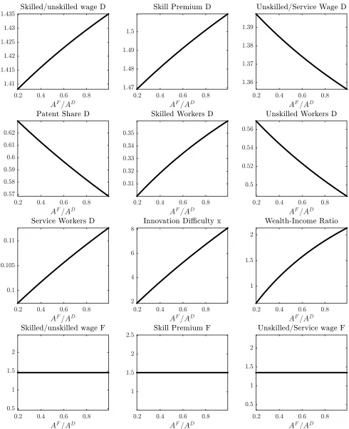
Proposition 2 A reduction in the innovation technology gap AD/AF produces the following
effects:
i. The domestic unskilled wage wD
L decreases, the relative skilled wage wDH/wLD increases
along with the fraction of the population acquiring education (lower θD
0 ).
ii. The fraction of sectors monopolized by domestic firms qD decreases.
iii. The fraction of the domestic labour force employed in personal servicesθD
LS increases and
the fraction of labour force employed in production decreases.
iv. It is harder to innovate successfully in the global economy: the innovation difficulty index,
x, increases.
v. Foreign skill and wage structure does not experience any change.
The effect of foreign technological competition on the skill and wage structure of the
domes-tic country works through two different channels: the international business-stealing channel
and the global competition channel. In providing the key economic intuitions, we focus on the
link between changes in the technology gap and changes in the relative wage of skilled workers.
As shown in section 3.1, the relative wage wHD/wDL is the key variable that determines the
whole wage and skill structure.
International business stealing. A reduction in the technology gap increases the
rela-tive innovation intensityIF/ID, thereby reducing the share of sectors with domestic leadership
qD. This is the business-stealing effect, typical of Schumpeterian models, in an open economy
environment with two innovating asymmetric countries. As foreign innovation technology
im-proves, foreign firms obtain global leadership in more sectors; as a consequence, production
shifts away from the home market, thereby leading to lower labour demand and lower wages
for unskilled production workers. Hence, a reduction in wLD directly leads to higher relative
triggering an increase in the incentive to innovate and in the demand for skilled workers which
further increases the relative skilled wage.14
Global competition effect. Better foreign innovation technology generates an increase
in the demand for skilled workers in the domestic country through its effect on the difficulty of
innovation. As foreign innovation becomes relatively more productive, the relative innovation
intensity IF/ID increases. Due to the technology gap, country D innovates more than F,
and since innovation technology (15) has decreasing returns at the country level, an increase
in IF/ID raises global innovation efficiency leading to higher innovation and growth. In our
semi-endogenous Schumpeterian growth model, steady-state quality growth is pinned down by
population growth: combining (24) and (20) we obtain the steady-state growth rate,
g = Q˙
Q = n
1−φ1
. (33)
The growth-enhancing effect of a lower international technology gap can then only be temporary,
and fades away in the long run due to the increase in the innovation difficulty index. Equilibrium
condition (24) implies that in steady state, domestic innovation ID decreases to exactly offset
the increase in foreign innovation.15 The skilled labour market clearing condition (22) tells us
then that, due to the increase in innovation difficulty, the domestic country is forced to devote
more labour resources to innovation, and this triggers an increase in skilled wages.16 We name
this the global competition effect: stronger foreign competition for innovation makes it harder
14Recall that the markup for country D firms is λ/wD L −1
/λ.
15Recall that our numeraire is the foreign unskilled wage, hence a reduction in ID must be
interpreted as a decline in domestic innovation rate measured in terms of foreign unskilled
wages.
16The skilled labour market clearing condition (22) can be written as H(θD
0 ) =
ID/AD1/(1−α)
x, where H(θD
0 ) is the supply of skilled workers. A reduction in AD/AF
re-duces θD
0 , thereby increasing H(θD0 ) - since dH(θ0D)/dθ0D < 0. For the market to clear, the
increase in the supply of skilled workers must be matched by an equivalent increase in the
for domestic firms to innovate in the global economy, thus forcing them to devote more (skilled)
labour to innovation.
Finally, because of the increase in the relative skilled wage wDH/wLD, skilled workers’ time
becomes more valuable, thus increasing the demand for service sector workers. The higher
demand, in turns, attracts more unskilled workers into service occupations, thereby increasing
the ability cutoff θD
LS. Since more people acquire education and become skilled (θD0 is lower)
and more unskilled workers choose to be employed in service occupations (θD
LS is higher), the share of unskilled workers in production shrinks.
As shown in the appendix, the equilibrium ability cutoff to acquire education for country
F can be obtained in closed form as a function of parameters, θ0F ≡θ¯0F(n, ρ, λ, η, φ1, φ, σ), and
is independent on innovation efficiency parametersAD and AF. Sinceθ0F is the key variable to
determine the wage structure, if changes in the relative innovation efficiency do not affect this
cutoff, labor market polarization remains unchanged. To interpret this result, recall that in this
economy the competitive fringe pinning down the equilibrium pricing of firms is represented
by the foreign country unit cost of production, the unskilled wage wF
L,which is our numeraire. As discussed above, a reduction in the technology gap AD/AF reduces the unskilled wage in
country D, increases the profits of its firms, boosting innovation and the demand for skilled
labor. In country F this mechanism does not operate: since the competitive fringe is foreign
unit cost, the markup of foreign firms is (λ−1)/λ, which implies that their profits are not
affected by the reduction in the technology gap. As a consequence, the business-stealing effect
does not lead to any change in the demand for skills, leaving the wage structure unaltered. In
the extended model that we use for quantitative analysis, we show that in the presence of trade
costs there exists a parameterization allowing the unit cost of both countries to potentially
represent the competitive fringe. Under this parameterization the neutrality result discussed
here breaks down, and changes in the technology gap affect polarization in both countries.
Finally, notice that the global competition effect on the wage structure is not operative either:
the increase in the difficulty index, which could potentially increase the demand for skills, is
In order to keep the analysis tractable and derive the final set of properties of our model, we
now assume that abilities are distributed uniformly. This assumption allows us to move from
predicting the effects of changes in the technology gap on the relative wages per units of skills,
to predicting the effects on average wages at the top, the middle, and the bottom of the skill
distribution.
Proposition 3 Under a uniform distribution of abilities, Γ(θ0K) = θ0K, a reduction in the
innovation technology gap AD/AF widens wage polarization in the domestic country:
i. The wage of average skilled workers relative to that of average unskilled production
work-ers, w˜DH/w˜LD, increases.
ii. The average wage of service sector workers relative to that of unskilled production workers,
˜
wD
S/w˜DL, increases.
As shown in Proposition 2, a reduction in the innovation technology gap increases the
rela-tive wage of skilled workerswD
H/wLF. This effect produces changes in the average ability of skilled and unskilled workers that can potentially offset its impact on the average skilled/unskilled
wage ratio ˜wD
H/w˜DL. On the one hand, as more people acquire education (lowerθD0 ), the average
quality of skilled workers eθDH declines. On the other hand, a lowerθ0D reduces the quality of
un-skilled workers employed in production while a higherθD
LS has the opposite effect. The relative strength of these forces determines the changes in the average quality of workers eθDH/eθDL. The
result above shows that, under uniform ability distribution, the overall effect of a reduction in
the technology gap on wage inequality in the upper tail of the skill distribution is positive.
Changes in the wage of service relative to production workers, ˜wD
S/w˜LD, are pinned down by the effects on the average quality of workers in these different occupations, as the wage per
unit of skills is the same for all unskilled workers. The increase in the cutoff, θD
LS,following the decline in the technology gap, increases the average quality of service workers, θeSD, but has an
ambiguous effect on the average quality of production workers, as we saw above. With uniform
ability distribution, the overall effect of lower technology gap on the relative service sector wage
by a reduction in the innovation technology gap increases wage polarization, benefiting skilled
workers and damaging workers in the middle of the skill distribution more than those at the
bottom.
5.1
Globalization and the wealth-income ratio: a Schumpeterian
view
Besides the predictions on the evolution of personal wage inequality, which tracks wage
differ-ence across individuals, our theory has implications for a different dimension of inequality, the
wealth to income ratio. The data reported in Figure 1 show that the increase in the wealth to
income ratio in the last decades is essentially due to the rise of financial assets, with housing
and non-financial assets being substantially constant. More than two thirds of financial assets
are represented by equities, the market value of corporations. Since the stock market value
of firms is the core engine of growth in the Schumpeterian framework, our model is a good
candidate to interpret the observed changes in the wealth-income ratio by linking them to the
dynamics of international technological competition.
In our model, country D’s aggregate wealth, denoted WD, coincides with the stock market
value of all the profit-generating firms in the economy, WD = ˜vDqD where ˜vD is the market
value of a generic monopolistic firm.17 As in the classical Schumpeterian theory (Aghion and
Howitt, 1992), the innovation free-entry condition (19) equates the expected value of a new
patent to the unit cost of innovation, here represented by the wage of a skilled labour unit. If
we multiply both sides by the share of skilled workers in the economy HD and use (22), the left
hand side becomes the aggregate value of the flow of new patents and the right side the flow of
savings in the economy, as shown in (30), ˜vDID =wD
HHD. Since by (24) and (33) ID =qDgλ¯,
17The value of a generic monopolistic quality leader is
˜
vD ≡ (c
D +cF) λ−wD L
ρ+(1−φ n
1)(λη−1−1) +
nφ1
1−φ1
we can write
˜
vDqD
| {z }
Wealth
gλ¯= wHDHD
| {z }
Savings
, (34)
where ¯λ = (λη−1 −1)−1 and g given by (33) are constant. The budget constraint (30) implies
that savings are SD = wD
HHD, and expressing aggregate savings SD as the product of the ‘endogenous’ marginal propensity to save multiplied by GDP, SD = sDYD, transforms (34)
into:
˜
βD ≡ W D
YD =
sD
gλ¯. (35)
This allows us to obtain the following result:
Proposition 4 A reduction in the innovation technology gapAD/AF raises countryD’s wealth
to national income ratio β˜D.
The economic intuition is the following. Since in our semi-endogenous growth model the
long-run growth rate is constant, the wealth to income ratio increases only if saving increases.
As aggregate saving equals total investment in innovation, and the incentive to innovate is
dictated by the market value of firms, the corporate wealth to income ratio is strictly increasing
in innovation. Faster innovation in our economy has only transitional effects on growth which
lead to persistently higher levels of saving and of the wealth-income ratio. Since in our model
a reduction in the technology gap increases the demand for skilled workers and innovation
spending in the leading country, it will also boosts the wealth to income ratio along with wage
polarization.
We can conclude that, our model captures the salient stylized facts of the US labour market
reported in Tables 1 and 2 and Figure 2, together with the evolution of the distribution of
global patents shown in Figure 3.
6
Quantitative analysis
In order to take the model to the data we generalize it along two dimensions. First, we remove
Secondly, we assume away free trade introducing trade barriers in the form of iceberg costs. We
then calibrate the parameters of the model to match some key statistics of the data discussed
in section 2, compute the numerical solution using the calibrated parameters and explore the
effects of our dimension of globalization on wage polarization and the wealth-income ratio.
Generalizations. We generalize the technology of our economy allowing skilled and unskilled
workers to be employed in both production and innovation. The production technology is
defined by the unit cost function,
ZK(wKL, wKH) = 1/zK wLKβ wHK1−β, for K =D, F.
We assume that the unit production cost in countryF is the numeraire, that isZF(wF
L, wHF)≡1. The innovation technology is described by the unit cost function
FK(wKL, wHK;AK)X(ω) = 1/AKX(ω) wLKϕ wHK1−ϕ, K =D, F,
where the difficulty index X(ω) = q(ω)/Qφ is the same as in the benchmark model. As
in the previous sections the technology gap is captured assuming AD > AF. The
country-specific production technology parameterzK is introduced for generality, and will not play any
particular role besides that of contributing to the numerical fit of the model in the calibration.
Assumption 2. (Factor Intensity): FHK/FLK > ZHK/ZLK: innovation is the skill intensive
activity. With the Cobb-Douglas technologies above, the factor bias of innovation is pinned
down by assuming β > ϕ.18
This assumption implies less extreme factor intensity compared to the baseline model. As we
will show, qualitatively it does not change the basic mechanisms: an increase in the incentive to
18This assumption guarantees a strictly concave transformation curve between the production
of goods and innovation probabilities. Any parameter configuration wih β 6= ϕ would avoid
a linear transformation curve. The upside is that we do not need the congestion externality
innovate will still increase the relative demand for skilled workers, and a reduction in a country’s
share of leadership will still reduce the relative demand for unskilled workers. Quantitatively,
factor intensity parameters β and ϕwill be important to determine the size of these changes.
We also introduce trade barriers in the form of iceberg costs. Firms need to ship τ > 1
units of goods in order to sell one unit abroad. In the presence of trade costs, the ”narrow gap”
assumption becomes τ ZD(wD
L, wDH)/λ < ZF(wFL, wHF) < ZD(wLD, wDH). As in the basic model, this allows quality leaders in country D to overcome a higher production cost by supplying a
higher quality good. Trade costs complicate the optimal pricing of firms compared to the basic
model. The optimal price choice of country F firms selling their product domestically (that
is, in country F market) pFd, and the optimal pricing of country D0s exporting firms (that is, selling in country F market) pDx leads to the same limit pricing,
pFd =λZF(wLF, wFH) =λ =λZF(wFL, wHF) = pDx.
In fact, in both cases, the limit price is anchored to the quality jump, λ, times the unit cost
of the world competitive fringe, which is country F0s production cost ZF = 1. Slightly more complex is the optimal strategy of firms selling in country D. In case ZD(wD
L, wDH) > τ, the relevant competitive fringe would still be countryF firms able to enter with the previous version
of the good. Then the optimal price choice of countryDfirms selling their product domestically
(that is, in country D market) pD
d and the price choice of country F exporting firms (that is, selling in country D market) pF
x yield the same limit pricing,
pDd =τ λZF(wFL, wHF) = τ λ=τ λZF(wLF, wFH) =pFx.
If instead ZD(wD
L, wDH) < τ, the relevant competitive fringe in country D market would be country D firms able to enter with the previous version of the good. Consequently, the
optimal price choice of country D firms selling their product domestically and of country F
exporting firms leads to the same limit pricing, pDd = λZD(wDL, wHD) = pFx. Finally, the two
pricing strategies coincide in the case ZD(wD