1
Efficient Binary Symbiotic Organisms Search Algorithm
Approaches for Feature Selection Problems
2
, Farhad Soleimanian Gharehchopogh
1Hekmat Mohmmadzadeh
Urmia,
Departent of Computer Engineering, Urmia Brach, Islamic Azad University,
1,2
IRAN.
Abstract
Feature selection is one of the main data preprocessing steps in machine learning. Its goal is to reduce the number of features by removing extra and noisy features. Feature selection methods must consider the accuracy of classification algorithms while performing feature reduction on a dataset. Meta-heuristic algorithms are the most successful and promising methods for solving this issue. The symbiotic organisms search algorithm is one of the successful meta-heuristic algorithms which is inspired by the interaction of organisms in the nature called Parasitism Commensalism Mutualism. In this paper, three engulfing binary methods based on the symbiotic organisms search algorithm are presented for solving the feature selection problem. In the first and second methods, several S-shaped and V-shaped transfer functions are used for binarizing the symbiotic organisms search algorithm, respectively. These methods are called BSOSS and BSOSV. In the third method, two new operators called BMP and BCP are presented for binarizing the symbiotic organisms search algorithm. This method is called EBSOS. The third approach presents an advanced binary version of the coexistence search algorithm with two new operators, BMP and BCP, to solve the feature selection problem, named EBSOS. The proposed methods are run on 18 standard UCI datasets and compared to base and important meta-heuristic algorithms. The test results show that the EBSOS method has the best performance among the three proposed approaches for binarization of the coexistence search algorithm. Finally, the proposed EBSOS approach was compared to other meta-heuristic methods including the genetic algorithm, binary bat algorithm, binary particle swarm algorithm, binary flower pollination algorithm, binary grey wolf algorithm, binary dragonfly algorithm, and binary chaotic crow search algorithm. The results of different experiments showed that the proposed EBSOS approach has better performance compared to other methods in terms of feature count and accuracy criteria. Furthermore, the proposed EBSOS approach was practically evaluated on spam email detection in particular. The results of this experiment also verified the performance of the proposed EBSOS approach. In addition, the proposed EBSOS approach is particularly combined with the classifiers including SVM, KNN, NB and MLP to evaluate this method performance in the detection of spam emails. The obtained results showed that the proposed EBSOS approach has significantly improved the accuracy and speed of all the classifiers in spam email detection.
Keywords: Efficient Binary Symbiotic, Feature selection, Classification, Optomization.
2
1. Introduction
In real-world problems, the existence of datasets with high dimensionality and also useless and extra data has made the process of analyzing these data challenging. Feature selection is one of the preprocessing steps in machine learning which can remove useless and irrelevant features from a dataset and find the ultimate subset of important features which leads to the better performance of machine learning algorithms[1, 2]. In fact, feature selection is an important and common method in data mining and machine learning for dimensionality reduction by eliminating irrelevant and redundant information from the dataset for achieving the optimal feature subset which leads to an increase in the speed and accuracy of classification algorithms[2, 3]. However, obtaining the optimal feature subset is posed as a complex optimization problem and conventional methods are unable to solve this problem. In fact, the goal of feature selection is finding a set of m features from the full set of n features which improves the performance of the learning algorithm in terms of learning speed or classification accuracy.
Until now, two frameworks, including search-based feature selection and correlation-based feature selection, have been proposed for solving the feature selection problem efficiently[2]. Search strategy and evaluation criterion are the two key components in the first set of methods. The search strategy specifies how the solution is generated for an optimal feature subset. Each generated solution is evaluated using a specified criterion. Of course, in this strategy, search methods try to work better in later iterations and the subset generation and evaluation process are repeated until a stopping criterion is met. Unlike the first set of methods, in the second set, the abundance, relationship, and correlation between features are used for identifying
3 Original feature set
Subset generation
Subset evaluation using learning algorithm
Performance measure
a
Original feature set
Feature subset selection
Classification algorithm Performance measure
b
S al ie nt f e at ur e s ubs et s e le c tion S al ie nt fe at ure s ubs etFig. 1. Action diagram (a) wrapper approach (b) filter approach[5].
The researchers have found out[4-9] that coating-based methods obtain better results compared to filter-based methods because they utilize the classification algorithm in their evaluation model. Coating models take advantage of meta-heuristic algorithms. Of course, nowadays, metaa-heuristic algorithms have proven themselves useful for most complex computational and optimization problems. These efficient and reliable methods are for finding near-optimal solutions with a reasonable computational cost. Of course, most of these algorithms are inspired by the behavior of creatures, animals’ hunting, or nature[10, 11]. At the beginning of meta-heuristic algorithm generations, they use exploration to generate new solutions and try to gradually decrease exploration as the generation comes closer to its end. On the other hand, they use exploitation to generate new solutions around the solutions they have already discovered. Therefore, meta-heuristic algorithms use the two exploration and exploitation operations to prevent being trapped in a local minimum and converge to the target.
4
to present a coating-based method for moving in the binary space. Furthermore, in the third method, two new operators called BMP and BCP were presented for making the advanced binary version of the symbiotic organisms search algorithm called EBSOS. In the EBSOS approach, our goal is to apply some changes to the structure of the operators of the symbiotic organisms search algorithm based on various new operators while keeping the rules present in the base symbiotic organisms search algorithm. In this method, of course, we have tried for exploration and exploitation to be upheld.
In the rest of this paper, binary versions of various meta-heuristic algorithms are reviewed in section 2. In section 3, the fundamental concepts of the symbiotic organisms search algorithm and its steps are explained in detail. In section 4, the three proposed binary approaches based on the symbiotic organisms search algorithm are presented. In section 5, the efficiency and performance of the proposed approaches will be tested. In the final section of the paper, the overall conclusion and future work will be presented.
2. Previous Work
In this section, we will review the papers about feature selection. Of course, we have comprehensively described the methods of transforming continuous meta-heuristic algorithms to binary in table 1. and described the differences and operators of our proposed methods in the end as well. Since our proposed method is a coating-based method, we will mostly review papers which are coating-based and have used different transfer functions. In 2013, a particle swarm algorithm based on two V-Shaped and S-shaped transfer functions was presented by Mirjalili et al.[12]. The proposed method was run on 2005 benchmark functions and the results of the proposed method were promising compared to other methods. In another research in 2013, a binary cuckoo search algorithm was presented for feature selection[13]. In this study, only the S-shaped transfer function was used for transforming the continuous space to binary. Finally, the proposed method was run on two datasets which showed that the proposed method performs better than base binary algorithms like binary bat algorithm, binary particle swarm, binary firefly algorithm, and binary gravitational search algorithm.
Table 1: Investigating some research on the problem of feature selection with binary continuous space conversion methods
Suggested method for conversion Meta-heuristic algorithm
Authors Reference
V-shaped S-shaped
Particle swarm optimization
(Mirjalili & Lewis, 2013) [12]
S-shaped
Cuckoo search algorithm
(Rodrigues et al., 2013)
[13]
V-shaped S-shaped
Bat algorithm
(Mirjalili, Mirjalili, & Yang, 2014)
[14]
S-shaped Crossover
Grey wolf optimization
(Emary, Zawbaa, & Hassanien, 2016b)
[8]
V-shaped S-shaped Crossover
Ant lion optimization
(Emary, Zawbaa, & Hassanien, 2016a
5
Crossover Mutation
Whale optimization algorithm
(Mafarja & Mirjalili, 2018)
[15]
Types of-V-shaped Types of-S-shaped
Binary salp swarm algorithm
(Faris et al., 2018)
[6]
V-shaped S-shaped
Butterfly optimizationalgorithm
(Arora & Anand, 2019)
[4]
V-shaped S-shaped Crossover
Mutation
Grasshopper optimisation algorithm
(Mafarja et al., 2019)
[1]
Types of-V-shaped Types of-S-shaped New Operator(BCP) New operator(BMP)
Crossover Mutation
Symbiotic Organisms Search This Article
-
In[14], a binary bat algorithm based on two V-shaped and S-shaped transfer functions was presented by Mirjalili et al. in 2014. Experiments were carried out on 22 benchmark functions and the results showed that the binary bat algorithm performed significantly better compared to the genetic and particle swarm algorithms. Also, the proposed algorithm performed better in real-world problems as well.
In 2016, two binary grey wolf optimization approaches were presented for feature selection[8]. In the first approach, the composition operator is used for updating the operators of the grey wolf optimization algorithm. In the second approach, the sigmoidal function is used to move the grey wolf optimization algorithm in the binary space and finally, random thresholding is carried out to convert the solutions to binary. To evaluate and compare the proposed and other methods, 18 different datasets from the UCI repository were used. The simulation results indicated the superiority of the first method more. Also, in another research, a binary ant lion algorithm was presented for feature selection[7]. In this research, two types of approaches were studied for binarizing the binary ant lion algorithm. In the first approach, the composition operator was used and in the second approach, the S-shaped and V-shaped transfer functions were used. The experiments we applied on 21 datasets and the results showed that the proposed algorithm based on the composition operator has presented acceptable results.
6
were presented in this study as well. In the first approach, eight binary transfer functions are used for converting the continuous version of the Salp swarm algorithm to binary. In the second approach, the composition operator was used to replace the ordinary operator and increasing the exploration behavior of the algorithm in addition to the transfer functions. Finally, different tests verify the superiority of the proposed algorithms.
In the most recent research in 2019, Arora and Anand presented two binary approaches to the impulse optimization algorithm[4]. In the first approach, the S-shaped transfer function is used to
transform the continuous space to binary while in the second approach, the V-shaped transfer function is used for transforming the continuous space to binary. To evaluate and compare the performance of the proposed algorithms, more than 21 datasets from the UCI repository were used. Experimental results showed that the approach based on the S-shaped transfer function performs better than the V-shaped transfer function. In addition, the proposed method has performed better compared to other algorithms in terms of improving the classification accuracy. In another research, two different approaches of the Grasshopper Optimization Algorithm were presented by Mafarja et al. for solving the feature selection problem[1]. The first approach is based on the Sigmoid and V-shaped transfer functions and are named BGOA-S and BGOA-V respectively. The second proposed approach combines the best obtained solutions and also a mutation operator is utilized for increasing the exploration phase in the BGOA algorithm. Finally, the second approach is called BGOA-M. the proposed methods were evaluated using 25 standard UCI datasets and compared to 8 coating-based meta-heuristic approaches and six well-known filter-based methods. Test results show the advantage of BGOA and BGOA-M methods compared to other similar techniques.
As seen in table 1, researchers have used different meta-heuristic algorithms for solving binary problems, including feature selection, and in most studies, it is tried to use transfer or transform functions in the main procedures of each meta-heuristic algorithm to move them in the binary space. In some versions, they have only used an S-shaped transfer function while in others, they have used only the V-shaped transfer function. Of course, in some studies, both the S-shaped and V-shaped functions have been used for presenting the binary version of meta-heuristic algorithms[4, 16, 17]. Of course, in different studies, different versions of the S-shaped and V-shaped functions are used simultaneously. Finally, some researchers have used the mutation and crossover operators for presenting the binary version of meta-heuristic functions[4, 16, 17]. However, each one of the S-shaped and V-S-shaped functions might have its advantages and one might outperform the other in an algorithm depending on the procedures of the algorithm. Also, the mutation and crossover operators can be suitable operators for transforming continuous meta-heuristic algorithms to the binary version. However, if its exploration and exploitation are not tuned correctly, it will lead to the poor performance of the considered algorithm and occasional premature or slow convergence. Therefore, in our proposed method, we have considered the symbiosis search as the proposed method, which is a powerful algorithm for solving optimization problems, and used a different version of the S-shaped and V-shaped functions simultaneously for moving in the binary search space. In addition, in the third method, two new operators called BMP and BCP are presented for binarizing the symbiosis organisms search algorithm.
7
In this section, we will briefly study the symbiotic organisms search algorithm. The readers can use references[18, 19] for more reading and advantages and limitations. The symbiotic organisms search algorithm is a meta-heuristic inspired by the opposition of organisms presented by Cheng and Prayogo in 2014 for solving optimization problems[19]. This algorithm starts working with an initial population called the ecosystem. In this ecosystem, a group of organisms is randomly generated in the search space and each organism is considered a solution for solving the optimization problem. Each one of the solutions or organisms has a fitness attributed to it. Furthermore, there are no parameters in this algorithm for tuning exploration and exploitation and this is done automatically. Also, since it uses optimal solutions of the current neighbor and the global solution through two commensalism and mutualism steps, it has good exploitation[18].
The main point in this algorithm is the way new solutions are generated. New solution generation is done by emulating the relationship or interaction of two organisms in the ecosystem. In this algorithm, the most prevalent or popular symbiosis relationship between two organisms in the environment is simulated which includes mutualism, commensalism, and parasitism. Figure 2. presents the most common symbiosis relationships in the environment, i.e. mutualism, commensalism, and parasitism.
(a): Mutualism (b): Commensalism (c): Parasitism
Fig. 2. Three main stages of symbiotic[18]
In figure 2., the main three steps of symbiosis are presented. In the mutualism step, both the organisms profit while in commensalism, only one organism profits but not the other. Finally, in the parasitism state of life, one organism profits while the other one gets harmed. In the following, first, the flowchart of the symbiosis organisms search algorithm is presented in figure 3. Then, each step of the algorithm is described comprehensively.
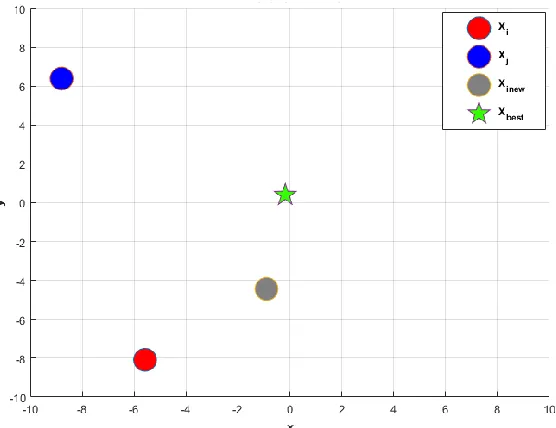
Mutualism Stage: in this stage, two organisms start a relationship and both will profit from this relationship. The relationship between bees and flowers can be mentioned which is presented in figure 2. part (a). In this step of the symbiotic organisms search algorithm, two organisms called Xi and Xj are chosen from the ecosystem on random and both organisms profit or update according to equations 1 and 2.
( 1 )
𝑋𝑖𝑛𝑒𝑤= 𝑋𝑖+ 𝑟𝑎𝑛𝑑 × (𝑋𝑏𝑒𝑠𝑡− 𝑀𝑢𝑡𝑢𝑎𝑙_𝑉𝑒𝑐𝑡𝑜𝑟 × 𝐵𝐹1)
( 2 )
8
( 3 )
𝑀𝑢𝑡𝑢𝑎𝑙_𝑉𝑒𝑐𝑡𝑜𝑟 =𝑋𝑖+ 𝑋𝑗 2
In equations 1 and 2, 𝐵𝐹1 and 𝐵𝐹2 represent the profit coefficient of the two organisms and each organism’s profit might be different than the other. Therefore, in this algorithm, 𝐵𝐹1 and 𝐵𝐹2 are determined randomly between 1 and 2. Also, rand is a random vector of numbers between zero and one. 𝑀𝑢𝑡𝑢𝑎𝑙_𝑉𝑒𝑐𝑡𝑜𝑟, the mutual vector, represents the relationship between organisms Xi and Xj. Also, Xbest represents the best organism in the ecosystem.
Commensalism Stage: in this stage, two organisms start a relationship and one of the organisms will profit from this relationship while the other one is not affected at all. The relationship between sticky fish and sharks can be mentioned which is presented in figure 2. part (b). In this step of the symbiotic organisms search algorithm, two organisms name Xi and Xj are chosen from the ecosystem on random and organism Xj is updated according to equation 4.
( 4 )
𝑋𝑖𝑛𝑒𝑤= 𝑋𝑖+ 𝑟𝑎𝑛𝑑(−1.1) × (𝑋𝑏𝑒𝑠𝑡− 𝑋𝑗)
In equation 4, rand is a random vector of numbers between -1 and 1 while Xbest represents the best organism in the ecosystem.
Parasitism Stage: in this stage, two organisms enter a relationship where one of the organisms profits from this relationship while the other is damaged by it. The relationship between the Malaria disease which is transmitted to humans by Malaria mosquitos which is presented in figure 2. part (c). In the symbiotic organisms search algorithm, an organism 𝑋𝑗 is chosen on random and like the Malaria mosquito, it acts like a parasite by creating an artificial parasite “Parasite-Vector”. The parasite is created in the space by the multiplication of organism 𝑋𝑗. Parasite-Vector tries to replace
9
Number of organisms (eco_size), initial ecosystem, termination criteria, num_iter=0, num_fit_eval=0, max_iter, max_fit_eval
num_iter=num_iter+1; i = 1
Identify best organism (Xbest)
Mutualism Phase
CommensalismPhase
ParasitismPhase
i = eco_size?
Terminal Condition?
End
yes
yes No
No
i = i + 1
Start
Ecosystem Initialization
Fig. 3. Flowchart of the SOS algorithm[18, 20]
4. Proposed Method
10
most successful transfer functions from the continuous to the binary state. In addition, we will present a different version by making some modifications to the structure of the symbiotic organisms search algorithm procedures. In this version, some new operators are used. In the rest of this section, we describe the proposed method in three different subsections. In section 4.1, a binary version of the symbiotic organisms search algorithm based on the Sigmoid function will be presented. In this approach, four different functions are used for moving the symbiotic organisms search algorithm in the binary space. Finally, after experiments, an S-shaped function is considered as the transfer function from the continuous space to the binary space. In section 4.2, a binary version of the symbiotic organisms search algorithm based on the V-shaped function will be presented. In this approach, four different V-shaped functions are presented for moving the symbiotic organisms search algorithm in the binary space. Finally, after some experiments, a V-shaped function is used as the final transfer function between the continuous and binary space. In section 4.3, a different binary version based on altering the procedures of the symbiotic organisms search algorithm will be presented which uses new operators presented to improve the exploration and exploitation of the proposed algorithm. Finally, in section 4.4, a valid multi-objective function is presented for feature reduction and improving the classification accuracy.
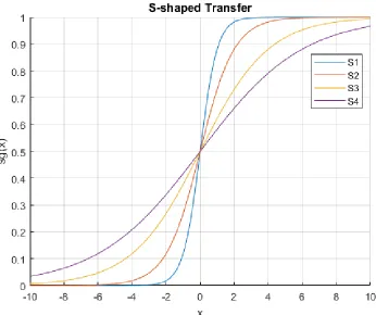
Fig. 4. Graphical representation of the S-shaped transfer function types
4.1 Binary Symbiotic Organisms Search Algorithm based on the S-shaped base function (BSOSS)
11
Sigmoid or S-shaped function[4, 12, 21] is a transfer function which has been proven to be effective for transforming the continuous space to binary by many researchers. We used four well-known functions for binarization as well. These famous Sigmoid functions are presented in table 2 along with their formula. Also, the graphical state of these four functions is presented comprehensively in figure 4.
Table 2: Types of Sigmoid Transfer Function Function
name
Transfer function
Transfer function in coexistence search algorithmS1 𝑠𝑔(𝑥) = 1
1 + e−2𝑥 𝑠𝑔(𝑆𝑂𝑆𝑖
𝑑(𝑡)) = 1
1 + e−2𝑆𝑂𝑆𝑖𝑑(𝑡)
S2 𝑠𝑔(𝑥) = 1
1 + e−𝑥 𝑠𝑔(𝑆𝑂𝑆𝑖
𝑑(𝑡)) = 1
1 + e−𝑆𝑂𝑆𝑖𝑑(𝑡)
S3 𝑠𝑔(𝑥) = 1
1 + e(−𝑥2)
𝑠𝑔(𝑆𝑂𝑆𝑖𝑑(𝑡)) =
1
1 + e(−
𝑆𝑂𝑆𝑖𝑑(𝑡) 2 )
S4 𝑠𝑔(𝑥) = 1
1 + e(−𝑥3)
𝑠𝑔(𝑆𝑂𝑆𝑖𝑑(𝑡)) = 1 1 + e(−
𝑆𝑂𝑆𝑖𝑑(𝑡) 3 )
Therefore, in the BSOSS approach, four S1, S2, S3, and S4 transfer functions are used for transforming the continuous symbiotic organisms search algorithm to the binary form. In table 2, 𝑆𝑂𝑆𝑖𝑑 is the continuous value of solution 𝑖 among the population of the symbiotic organisms search algorithm in dimension 𝑑 at iteration 𝑡. According to the output obtained from figure 4., it is seen that the output of four shaped functions are continuously between 0 and 1. After using four S-shaped functions, thresholding is carried out and the best case in meta-heuristic algorithms is to use a random function for thresholding. Finally, in the S-shaped functions, an organism can be updated in the next iteration using equation 5.
( 5 ) 𝑆𝑂𝑆𝑖𝑑(𝑡 + 1) = {
0𝑖𝑓𝑟𝑎𝑛𝑑(0.1) < 𝑠𝑔(𝑆𝑂𝑆𝑖𝑑(𝑡))
1𝑖𝑓𝑟𝑎𝑛𝑑(0.1) ≥ 𝑠𝑔(𝑆𝑂𝑆𝑖𝑑(𝑡))
In equation 5., 𝑆𝑂𝑆𝑖𝑑 is the position of solution 𝑖 in the population at iteration 𝑡 in dimension 𝑑 of the symbiotic organisms search algorithm. Also, 𝑟𝑎𝑛𝑑(0.1) is a number between zero and one from a uniform distribution. According to this equation, all the solutions present in the symbiotic organisms search algorithm will be transformed to binary. In the following, we added four S-shaped functions to the symbiotic organisms search algorithm as presented in the pseudo-code in figure 5.
BSOSS Algorithm
01: Define S-Shaped Transfer function S1,S2,S3,S4 according to Table(2)
02: Determining initial parameter
03: Generate an ecosystem Xi (i=1... EcoSize) with random Xi∈ random 0,1
04: Calculate Objective function according to Equations (10) 05: Select one S-Shaped Transfer[1]
12 07: For i = 1:EcoSize
08: Find the 𝑋𝑏𝑒𝑠𝑡in the ecosystem 09: % Mutualism Phase
10: Randomly select X𝑗 (Xj ≠ Xi)
11: Determine 𝑀𝑢𝑡𝑢𝑎𝑙_𝑉𝑒𝑐𝑡𝑜𝑟 and 𝐵𝐹1 ,𝐵𝐹2
12: calculation 𝑋𝑖𝑛𝑒𝑤 and 𝑋𝑗𝑛𝑒𝑤according to Equations (1) and (2)
13: Convert Continuous(𝑋𝑖𝑛𝑒𝑤) to Binary(𝐵𝑋𝑖𝑛𝑒𝑤) using transfer S-shaped according to Equations (5) and
Table(2)
14: Convert Continuous(𝑋𝑗𝑛𝑒𝑤) to Binary(𝐵𝑋𝑗𝑛𝑒𝑤) using transfer S-shaped according to Equations (5) and
Table(2)
15: Replace 𝑋𝑖 with 𝐵𝑋𝑖𝑛𝑒𝑤(if 𝐵𝑋𝑖𝑛𝑒𝑤gives better fitness) and 𝑋𝑗 with 𝐵𝑋𝑗𝑛𝑒𝑤(if 𝐵𝑋𝑗𝑛𝑒𝑤gives better
fitness)
13: %Commensalism Phase
16: Randomly select Xj (Xj ≠ Xi)
17: calculation 𝑋𝑖𝑛𝑒𝑤 according to Equation (4)
18: Convert Continuous(𝑋𝑖𝑛𝑒𝑤) to Binary(𝐵𝑋𝑖𝑛𝑒𝑤) using transfer S-shaped according to Equations (5) and
Table(2)
19: Replace 𝑋𝑖 with 𝐵𝑋𝑖𝑛𝑒𝑤(if 𝐵𝑋𝑖𝑛𝑒𝑤gives better fitness)
20: % Parasitism Phase
21: Randomly select Xj (Xj ≠ Xi)
22: Generate Parasite_Vector from organism Xi
23: Convert Continuous(Parasite_Vector ) to Binary using transfer S-shaped according to Equations (5) and
Table(2)
24: Replace 𝑋𝑗 with BParasite_Vector (if BParasite_Vectorgives better fitness)
25: end for
26: Save 𝑋𝑏𝑒𝑠𝑡 in each iteration 27: End while
28: Print 𝑋𝑏𝑒𝑠𝑡
Fig. 5. Pseudo-code of BSOSS approach
In figure 5., the pseudo-code of the BSOSS approach based on four S-shaped functions is presented. According to line (01) of the pseudo-code, first, each transfer function is defined in the simulation environment. Then, setting the parameters and generating the initial population is done randomly in lines (02:03). In line (04), the definition of the target feature selection function defined in subsection 4.3 is implemented. In line (05), one of the S-shaped transfer functions gets selected for transforming the continuous space to binary. In lines (06:28), the main loop of the BSOSS approach which includes mutualism, commensalism, parasitism, and binarization phases is run. In lines (12:13, 18, and 23), new changes are made so that two 𝑋𝑖𝑛𝑒𝑤 and 𝑋𝑗𝑛𝑒𝑤 solutions are transformed to
the binary space before being evaluated by the target function and two new solutions 𝐵𝑋𝑖𝑛𝑒𝑤 and
𝐵𝑋𝑗𝑛𝑒𝑤 are created. In line (18), 𝑋𝑖𝑛𝑒𝑤 generated in the commensalism step is transformed to the
binary space before being evaluated by the target function and the new solution called 𝐵𝑋𝑖𝑛𝑒𝑤 is
13
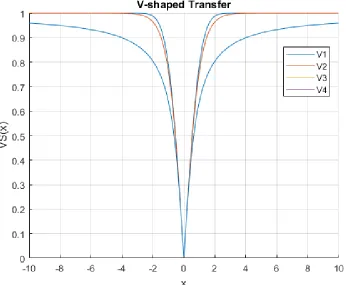
Fig. 6.Graphical view of the V-shaped transfer function types
4.2 Binary Symbiotic Organisms Search Algorithm Based on the V-shaped Transfer Function (BSOSV)
In this section, the new BSOSV approach consisting of multiple V-shaped transfer functions is presented for binarizing the symbiotic organisms search algorithm for solving the feature selection problem. The Tan hyperbolic or V-shaped function is another transfer function for binarizing meta-heuristic algorithms presented by Rashedi et al. in 2010[22] and has been approved by many researchers[1, 10, 12, 22]. In this paper, we used four well-known V-shaped functions for binarization. These four famous V-shaped functions are presented in table 3. along with their equations. Also, the graphical state of these functions is comprehensively presented in figure 6.
Table 3: V-shaped transfer function types
Function name
Transfer function
Transfer function in coexistence search algorithmV1 𝑉𝑆(𝑥) = |erf(√𝜋
2 x)| 𝑉𝑆(𝑆𝑂𝑆𝑖
𝑑(𝑡)) = |erf(√𝜋
2 𝑆𝑂𝑆𝑖
𝑑(𝑡))|
14
V3 𝑉𝑆(𝑥) = | 𝑥
√1 + 𝑥2| 𝑉𝑆(𝑆𝑂𝑆𝑖
𝑑(𝑡)) = || 𝑆𝑂𝑆𝑖𝑑(𝑡)
√1 + 𝑆𝑂𝑆𝑖𝑑(𝑡)2
||
V4
𝑉𝑆(𝑥)
= |2
𝜋𝑎𝑟𝑐 tan( 𝜋 2𝑥)|
𝑉𝑆(𝑆𝑂𝑆𝑖𝑑(𝑡)) = |2
𝜋𝑎𝑟𝑐 tan( 𝜋 2𝑆𝑂𝑆𝑖
𝑑(𝑡))|
In the BSOSV approach, four V1, V2, V3, and V4 transfer functions are used for transforming the continuous symbiotic organisms search algorithm to the binary form. We will act the same way for this transfer function as we did for the S-shaped transfer function where after applying four V-shaped transfer functions, thresholding takes place. Finally, in the V-V-shaped functions, an organism can be updated in the next iteration using equation 6.
( 6 ) 𝑆𝑂𝑆𝑖𝑑(𝑡 + 1) = {
0𝑖𝑓𝑟𝑎𝑛𝑑(0.1) <𝑉𝑆(𝑆𝑂𝑆𝑖𝑑(𝑡))
1𝑖𝑓𝑟𝑎𝑛𝑑(0.1) ≥𝑉𝑆(𝑆𝑂𝑆𝑖𝑑(𝑡))
All the details of equation 6. are like equation 5. with only the difference that we will use the V-shaped transfer function here. Later, we added the four V-V-shaped functions to the symbiotic organisms search algorithm as presented by the pseudo-code in figure 7.
BSOSV Algorithm
01: Define V-Shaped Transfer function V1,V2,V3,V4 according to Table(3)
02: Determining initial parameter
03: Generate an ecosystem Xi (i=1... EcoSize) with random Xi∈ random 0,1
04: Calculate Objective function according to Equations (10) 05: Select one S-Shaped Transfer{V1,V2,V3,V4}
06: while (t < MaxIt)
07: For i = 1:EcoSize
08: Find the 𝑋𝑏𝑒𝑠𝑡in the ecosystem 09: % Mutualism Phase
10: Randomly select X𝑗 (Xj ≠ Xi)
11: Determine 𝑀𝑢𝑡𝑢𝑎𝑙_𝑉𝑒𝑐𝑡𝑜𝑟 and 𝐵𝐹1 ,𝐵𝐹2
12: calculation 𝑋𝑖𝑛𝑒𝑤 and 𝑋𝑗𝑛𝑒𝑤according to Equations (1) and (2)
13: Convert Continuous(𝑋𝑖𝑛𝑒𝑤) to Binary(𝐵𝑋𝑖𝑛𝑒𝑤) using transfer V-shaped according to Equations (6) and
Table(3)
14: Convert Continuous(𝑋𝑗𝑛𝑒𝑤) to Binary(𝐵𝑋𝑗𝑛𝑒𝑤) using transfer V-shaped according to Equations (6) and Table(3)
15: Replace 𝑋𝑖 with 𝐵𝑋𝑖𝑛𝑒𝑤(if 𝐵𝑋𝑖𝑛𝑒𝑤gives better fitness) and 𝑋𝑗 with 𝐵𝑋𝑗𝑛𝑒𝑤(if 𝐵𝑋𝑗𝑛𝑒𝑤gives better
fitness)
13: %Commensalism Phase
16: Randomly select X𝑗 (Xj ≠ Xi)
17: calculation 𝑋𝑖𝑛𝑒𝑤 according to Equation (4)
18: Convert Continuous(𝑋𝑖𝑛𝑒𝑤) to Binary(𝐵𝑋𝑖𝑛𝑒𝑤) using transfer V-shaped according to Equations (6) and
Table(3)
19: Replace 𝑋𝑖 with 𝐵𝑋𝑖𝑛𝑒𝑤(if 𝐵𝑋𝑖𝑛𝑒𝑤gives better fitness)
15 21: Randomly select X𝑗 (Xj ≠ Xi)
22: Generate Parasite_Vector from organism Xi
23: Convert Continuous(Parasite_Vector ) to Binary using transfer V-shaped according to Equations (6) and Table(2)
24: Replace 𝑋𝑗 with BParasite_Vector (if BParasite_Vectorgives better fitness)
25: end for
26: Save 𝑋𝑏𝑒𝑠𝑡 in each iteration 27: End while
28: Print 𝑋𝑏𝑒𝑠𝑡
Fig. 7. BSOSV approach pseudo-code
In figure 7., the pseudo-code of the BSOSV approach based on four V-shaped functions is presented. Description of this pseudo-code is similar to the pseudo-code of the BSOSS approach with the difference that in this approach, four V-shaped functions including V1, V2, V3, and V4 are used for transforming the continuous symbiotic organisms search algorithm to the binary form.
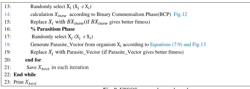
4.3 Efficient Binary SOS (EBSOS)
In this part, the Efficient Binary Symbiotic Organisms Search algorithm is presented. In this paper, we have named this approach EBSOS. In this approach, some major changes have been applied to transform the mutualism, commensalism, and parasitism steps from the continuous form to the binary form. Transforming the mutualism step from continuous to binary is so that first, the binary mutual vector (BMV) is presented and then, the binary for of the mutualism step along with its changes and pseudo-code is named BMP. Transforming the commensalism step from the continuous form to the binary form is such that organism Xi follows two general rules in this step. In the first rule, organism Xi moves more toward Xbest and in the second rule, organism Xi takes solution Xj into consideration and in this step, a new operator called BCP is defined. Transforming the parasitism step from continuous to the binary form is such that first, solution Xi is considered as the Parasite_Vector. Then, some dimensions of Parasite_Vector are chosen on random and these random indices are saved in idx_random. Finally, entries in these random indices are refilled with random numbers in [0, 1]. In the following, each new step of the algorithm is described in detail and its equations are presented. Also, the pseudo-code is presented in figure 8.
EBSOS Algorithm
01: Determining initial parameter
02: Generate an ecosystem Xi (i=1... EcoSize) with random Xi∈ random 0,1 03: Calculate Objective function according to Equations (10)
04: while (t < MaxIt)
05: For i = 1:EcoSize
06: Find the 𝑋𝑏𝑒𝑠𝑡in the ecosystem 07: % Mutualism Phase
08: Randomly select X𝑗 (Xj ≠ Xi)
09: Determine 𝐵𝑖𝑛𝑎𝑟𝑦𝑀𝑢𝑡𝑢𝑎𝑙_𝑉𝑒𝑐𝑡𝑜𝑟(𝐵𝑀𝑉) and 𝐵𝐹1 ,𝐵𝐹2 according to Fig.9
10: calculation 𝑋𝑖𝑛𝑒𝑤 and 𝑋𝑗𝑛𝑒𝑤according to Binary Mutualism Phase(BMP) Fig.10
11: Replace 𝑋𝑖 with 𝐵𝑋𝑖𝑛𝑒𝑤(if 𝑋𝑖𝑛𝑒𝑤gives better fitness) and 𝑋𝑗 with 𝑋𝑗𝑛𝑒𝑤(if 𝑋𝑗𝑛𝑒𝑤gives better
fitness)
16 13: Randomly select Xi (Xj ≠ Xi)
14: calculation 𝑋𝑖𝑛𝑒𝑤 according to Binary Commensalism Phase(BCP) Fig.12 15: Replace 𝑋𝑖 with 𝐵𝑋𝑖𝑛𝑒𝑤(if 𝐵𝑋𝑖𝑛𝑒𝑤gives better fitness)
16: % Parasitism Phase
17: Randomly select X𝑗 (Xj ≠ Xi)
18: Generate Parasite_Vector from organism Xi according to Equations (7:9) and Fig.13 19: Replace 𝑋𝑗 with Parasite_Vector (if Parasite_Vectorgives better fitness)
20: end for
21: Save 𝑋𝑏𝑒𝑠𝑡 in each iteration 22: End while
23: Print 𝑋𝑏𝑒𝑠𝑡
Fig. 8. EBSOS approach pseudo-code
4.3.1 Changing the Assistance Stage From continuous to binary Mode
In this step, two organisms enter a relationship they will both profit from. The mutual vector is the first thing that needs to change in this step so that it is usable for the binary problem. Here, we first define the mutual vector such that it contains all the mutual points. Then, non-mutual points are chosen randomly from either one of 𝑋𝑖 or 𝑋𝑗 solutions. This operation is called the Binary Mutual Vector (BMV) and is presented in detail in figure 9.
0
1
1
1
0
0
0
0
0
1
1
1
0
0
1
0
1
1
1
0
0
0
1
0
Fig. 9. Reciprocal vector in binary mode (BMV)
According to figure 9, the new BMV operator is used for creating the mutual vector in the binary form. The next step is using 𝐵𝐹1 and 𝐵𝐹2 for creating or improving new solutions. In this step, we have considered 𝐵𝐹1 and 𝐵𝐹2 as the composition coefficients of the mutual vector with Xbest. This way, values of 𝐵𝐹1 and 𝐵𝐹2 determine the amount of composition with Xbest in the binary form. Finally, after obtaining the mutual vector and combining it with the best solution, new solutions
X𝑖𝑛𝑒𝑤 and X𝑗𝑛𝑒𝑤 are sometimes randomly affected by the new vector. Overall, we defined a new BMP operator in this step and we have presented it in the pseudo-code in figure 10.
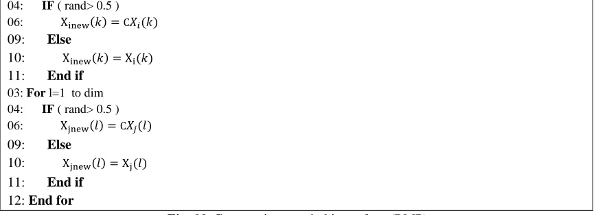
Binary Mutualism Phase: BMP
01:Xj= Randomly select X𝑗 (Xj ≠ Xi)
02:𝐵𝑀𝑉= calculation Mutual_Vector according to Fig.9 03: C𝑋𝑖= HybridBMV(𝐵𝑀𝑉. 𝑋𝑏𝑒𝑠𝑡. 𝐵𝐹1)
17 04: IF ( rand> 0.5 )
06: Xinew(𝑘) =C𝑋𝑖(𝑘)
09: Else
10: Xinew(𝑘) = Xi(𝑘)
11: End if 03: For l=1 to dim 04: IF ( rand> 0.5 ) 06: Xjnew(𝑙) =C𝑋𝑗(𝑙)
09: Else
10: Xjnew(𝑙) = Xj(𝑙)
11: End if
12: End for
Fig. 10. Cooperation step in binary form(BMP)
As seen in figure 10, first, organism X𝑗 is chosen randomly and then, organism X𝑖 and X𝑗 are combined with organism X𝑏𝑒𝑠𝑡 according to 𝐵𝐹1 and 𝐵𝐹2 and create two new solutions called 𝑐𝑋𝑖 and 𝑐𝑋𝑗. These two solutions will cause fundamental changes in organisms 𝑋𝑖 and 𝑋𝑗. Since we face the binary space in the new BMP operator, 𝑋𝑖𝑛𝑒𝑤 will use solution 𝑐𝑋𝑖 with a 50 percent chance. Otherwise, it uses solution 𝑋𝑖. Also, 𝑋𝑗𝑛𝑒𝑤 will use solution 𝑐𝑋𝑗 with a 50 percent chance and otherwise, it will use solution 𝑋𝑗. Of course, we have used a new suitable function for the binary form which is presented in figure 11.
01: Function HybridBMV(BMV,Xbest,BF) 02: n=dim(BMV);
03:Xnew=empty array(1,n); 04: For k=1:n
05: IF(rand<BF) 06: Xnew (k)=Xbest (k); 07: else
08: Xnew (k)=BMV(k); 09: End IF
10: End For
11: End Function
Fig. 11. New suitable function HybridBMV to combine function by BF
As presented in figure 11, in the first line, the best solution function gets the intended mutual vector and BF or profit from the input. Then, it tries to use the best solution and the binary mutual vector (BMV) to create new solutions according to BF. In line 4, the condition is set according to BF where the higher BF is, the new solution will use the best solution more. Otherwise, it uses the binary mutual vector (BMV) to create new solutions. Of course, variable BF here is between zero and one.
4.3.2 Transforming the commensalism step from continuous to binary
In this step, two organisms begin a relationship where one organism profits from this relationship and the other one is not affected by it. In the continuous form of mutualism, it is tried for organism
-18
1 and 1 adds more random moves to this step. We ran the continuous form of the SOS algorithm on MATLAB software. A sample solution along with its movement is depicted in figure 12.
Fig. 12. An example of the Xi movement in the food phase
As seen in figure 12, organism Xi follows two general rules. In the first rule, organism Xi moves more towards Xi while in the second rule, organism Xi considers solution Xj at the same time. We considered these rules in the binary commensalism step as well and defined them as a new operator called BCP. This operator is presented in the new pseudo-code in figure 13.
Binary Commensalism Phase: BCP 01:Xj= Randomly select X𝑗 (Xj ≠ Xi)
02:Xbest= Find the 𝑋𝑏𝑒𝑠𝑡in the ecosystem
03: For k=1 to dim 04: IF ( rand> 0.5 )
06: Xinew(𝑘) = Xbest(𝑘)
07: ElseIf ( rand> 0.5 ) 08: Xinew(𝑘) = Xj(𝑘) 09: Else
10: Xinew(𝑘) = Xi(𝑘) 11: End if
12: End for
Fig. 13. Binary Commensalism Phase (BCP)
As seen in figure 13, a random organism Xj is selected on random first. Then, organism Xi improves using this organism Xjand Xbest according to the two specified rules. In this new BCP operator, since we are faced with the binary space, the new solution uses Xbest with a 50 percent chance. Otherwise, it might stay unchanged with a 50 percent chance or it uses solution Xj.
19
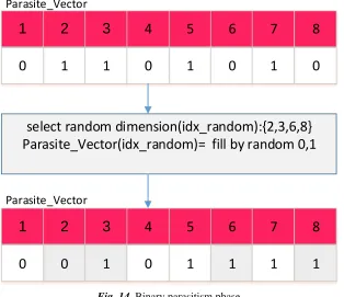
In the continuous symbiotic organisms search algorithm, the parasite or Parasite_Vector is created in the space by the multiplication of organism 𝑋𝑖. Parasite_Vector tries to replace 𝑋𝑗 in the ecosystem. Our binary version works similar to the continuous form but with the difference that Parasite_Vector grows in the binary space and tries to choose a random number between zero and one and leads to fundamental changes in the Prasite_Vector. To understand the parasitism step better, we have depicted it as figure 14.
2
3
1
4
5
6
7
8
1
1
0
0
1
0
1
0
2
3
1
4
5
6
7
8
0
1
0
0
1
1
1
1
Parasite_Vector
select random dimension(idx_random):{2,3,6,8}
Parasite_Vector(idx_random)= fill by random 0,1
Parasite_Vector
Fig. 14. Binary parasitism phase
In figure 14, first, solution 𝑋𝑖 is considered as the Prasite_Vector. Then, some dimensions of Parasite_Vector are chosen randomly and these random indices are saved in idx_random. Finally, entries corresponding to these random indices are replaced with random numbers in the [0, 1] interval. In this example, assuming we have a vector of dimension 8, indices 2, 3, 6, and 8 are chosen randomly and saved in idx_random. Finally, the binary parasitism phase can be defined as follows using equation 9:
( 7 )
Parasite − Vector = 𝑋𝑖
( 8 )
idxrandom= select random dimension(Parasite − Vector)
( 9 )
Parasite − Vector(idxrandom) = random0.1(1. size(idxrandom))
Furthermore, in this section, we have used the mutation operator to increase the exploration in the proposed approach which is applied to Parasite_Vector at the final step in order to achieve a better result.
20
The multi-objective function proposed for balancing the number of selected features in each solution (minimum) and classification accuracy (maximum) is presented in this section. This objective function is used in equation 10 for evaluating a solution in meta-heuristic algorithms.
𝐹𝑖𝑡𝑛𝑒𝑠𝑠 = 𝛼𝛾𝑅(𝐷) + 𝛽
|𝑅|
|𝑁| (10)
Where 𝛼𝛾𝑅(𝐷) represents the classification error of a classifier and |R| shows that the selected subset is multi-linear. Also, |N| is the number of all features available in the dataset while parameter α is the importance of classifier quality and parameter β is the length of the subset. The values of these two parameters are calculated according to α ∈ [0, 1] and β = (1 -α) which were adopted from research[7]. In this research, the initial value of α is considered to be 0.99. therefore, the value of β will be 0.01. Most researchers[9, 15, 23-25] use the simplest classification method, i.e. KNN[26]. We used this classifier for defining the objective function in the feature selection problem as well.
4 Evaluation and Results
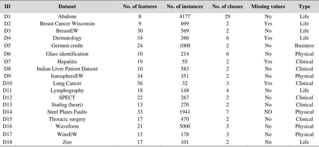
In this section, we have evaluated the proposed BSOSS, BSOSV, and EBSOS methods. All the tests in this section were run in MATLAB software on a system with a X GHz Core i5 processor and 8 gigabytes of RAM. To evaluate the proposed method, 18 feature selection datasets from the UCI[27] repository are used. The features of each dataset are comprehensively presented in table 4. Also, base algorithms like genetic algorithm[28], binary bat algorithm[29], binary particle swarm algorithm[30], binary flower pollination algorithm[31], binary grey wolf algorithm[8], binary dragonfly algorithm[32], and binary chaotic crow search algorithm[33] will be used for comparison with the final proposed approach (EBSOS).
Table 4. Dataset description
ID Dataset No. of features No. of instances No. of classes Missing values Type
D1 Abalone 8 4177 29 No Life
D2 Breast Cancer Wisconsin 9 699 2 Yes Life
D3 BreastEW 30 569 2 No Life
D4 Dermatology 34 366 6 Yes Life
D5 Germen credit 24 1000 2 No Business
D6 Glass identification 10 214 6 No Physical
D7 Hepatitis 19 55 2 Yes Clinical
D8 Indian Liver Patient Dataset 10 583 2 No Clinical
D9 IonosphereEW 34 351 2 No Physical
D10 Lung Cancer 56 32 3 Yes Clinical
D11 Lymphography 18 148 4 No Life
D12 SPECT 22 267 2 No Clinical
D13 Statlog (heart) 13 270 2 No Clinical
D14 Steel Plates Faults 33 1941 7 NO Physical
D15 Thoracic surgery 17 470 2 No Clinical
D16 Waveform 21 5000 3 No Physical
D17 WineEW 13 178 3 No Physical
21
In the rest of this section, we will first compare the methods based on the S-shaped function which are named S1, S2, S3, and S4 and then choose one of them which works better than the others as the final method based on the S-shaped function. Then, we will first compare the methods based on the V-shaped function called V1, V2, V3, and V4 and we will choose the one which works better than the others as the final method based on the V-shaped function. finally, we will compare the BSOSS, BSOSV, and EBSOS approaches. In the end, we will choose a method as the final approach and compare it to other methods. In addition to this, in the last section, we will present an applied study on an email span dataset to further evaluate the performance of the proposed algorithm.
5.1 Evaluation of S-shaped methods
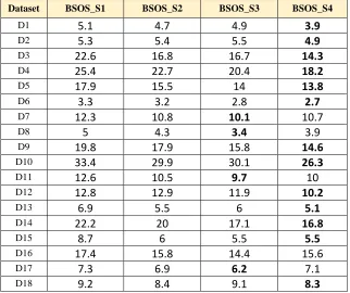
In this section, four S-shaped methods including S1, S2, S3, S4 are implemented on 18 datasets and the results are compared, and finally an S-shaped method is selected to compare the three approaches proposed in section (5-3). In these tests, the iterations and population are 50 and 10, respectively. We evaluate four S-shaped methods including S1, S2, S3, S4 in terms of mean feature number, classification accuracy and objective function convergence rate. In Table 5, four S-shaped methods including S1, S2, S3, S4 are shown in terms of the mean number of features.
Table 5: Comparison of four S-shaped methods based on the criterion of mean number of features
Dataset BSOS_S1 BSOS_S2 BSOS_S3 BSOS_S4
D1 5.1 4.7 4.9 3.9
D2 5.3 5.4 5.5 4.9
D3 22.6 16.8 16.7 14.3
D4 25.4 22.7 20.4 18.2
D5 17.9 15.5 14 13.8
D6 3.3 3.2 2.8 2.7
D7 12.3 10.8 10.1 10.7
D8 5 4.3 3.4 3.9
D9 19.8 17.9 15.8 14.6
D10 33.4 29.9 30.1 26.3
D11 12.6 10.5 9.7 10
D12 12.8 12.9 11.9 10.2
D13 6.9 5.5 6 5.1
D14 22.2 20 17.1 16.8
D15 8.7 6 5.5 5.5
D16 17.4 15.8 14.4 15.6
D17 7.3 6.9 6.2 7.1
22
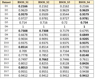
Table 5 shows the four methods based on the S-shaped transfer function in terms of the mean number of selected features with iteration number of 50. This experiment shows that the S4 performs best in terms of the average number of selected features, and the S3 sometimes does. But the S1 and S2 models have a relatively modest performance. In Table 6, four S-shaped methods including S1, S2, S3, S4 are presented in terms of accuracy criteria.
Table 6: Comparison of four S-shaped methods in terms of classification accuracy
Dataset BSOS_S1 BSOS_S2 BSOS_S3 BSOS_S4
D1 0.2166 0.2162 0.2162 0.2166
D2 0.9629 0.9629 0.9629 0.9629
D3 0.9579 0.9509 0.9544 0.9579
D4 0.9727 0.9781 0.9727 0.9781
D5 0.714 0.716 0.72 0.734
D6 1 1 1 1
D7 0.7308 0.7308 0.7179 0.6795
D8 0.6678 0.6781 0.6815 0.6849
D9 0.9034 0.9091 0.9205 0.9205
D10 0.9375 0.9375 0.9375 0.9375
D11 0.8514 0.8514 0.8378 0.8378
D12 0.709 0.7015 0.7164 0.7313
D13 0.7778 0.7852 0.7778 0.8148
D14 0.7497 0.7662 0.7446 0.7611
D15 0.8012 0.8255 0.8128 0.8426
D16 0.8013 0.7868 0.7888 0.7788
D17 0.9551 0.9551 0.9551 0.9438
D18 0.9412 0.9412 0.9412 0.9412
Table (6) shows the results associated with four methods which are based on the S-shaped transfer function in terms of classification accuracy with iteration 50. The test shows that the S4 is the best in terms of classification accuracy, and the S1 also performs better. However, the S2 and S3 models exhibit relatively poor performance in classification accuracy. Based on the results of feature selection and classification accuracy, it can be said that the S4 is the best model for both feature selection and classification accuracy. But other models have lost their performance in terms of accuracy and average selection. As a result, the S2 model is chosen as the final V-shaped approach.
5.2 Evaluation of V-shaped methods
23
Table 7: Comparison of four S-shaped methods based on the criterion of mean number of features
Dataset BSOS_V1 BSOS_V2 BSOS_V3 BSOS_V4
D1 4.8 4.4 4.5 4.3
D2 6.1 6.1 6.9 5.9
D3 16.6 17.2 15.8 18.3
D4 20.5 21.9 17.3 21.6
D5 13.9 12.8 13.6 11.5
D6 6.2 7 3.4 6.8
D7 9.3 9.3 7.9 10.9
D8 5.6 4.5 6.2 4.2
D9 16.6 16.5 16.8 19.5
D10 28.2 27.8 28.9 33.9
D11 9 10 9.8 8.8
D12 11.9 10.4 10.9 12.9
D13 7.1 7.1 7 6.2
D14 17.2 17.7 17.3 19.4
D15 7.2 7.1 8.7 8.7
D16 16.5 16.7 10.4 18.1
D17 6.5 6.5 6.7 6.2
D18 9.4 9.3 7.1 10.3
The results obtained based on Table (7) for comparing four V-shaped methods in terms of mean number of features show that the V4 and V3 models are the best in terms of the average number of selected features. Of course, the S1 and S2 models have shown average performance. The following four V-shaped methods including V1, V2, V3, V4 are compared in terms of accuracy criteria and their results are shown in Table (8).
Table 8: Comparison of four S-shaped methods in terms of classification accuracy
Dataset BSOS_V1 BSOS_V2 BSOS_V3 BSOS_V4
D1 0.2217 0.2217 0.219 0.2217
D2 0.9629 0.9629 0.9486 0.9657
D3 0.9439 0.9368 0.9158 0.9509
D4 0.9563 0.9672 0.7213 0.9454
D5 0.704 0.684 0.706 0.674
D6 0.9813 0.9813 0.972 0.9813 D7 0.6154 0.6026 0.5641 0.6154
D8 0.6849 0.6986 0.6644 0.7021
D9 0.9205 0.9034 0.8693 0.9148
D10 0.875 0.875 0.875 0.875
D11 0.7568 0.7568 0.6486 0.7973
D12 0.7388 0.7239 0.6045 0.7164
D13 0.7481 0.8011 0.6593 0.7407
D14 0.8074 0.7312 0.6375 0.8074
D15 0.8638 0.8255 0.8213 0.834
24
D17 0.9326 0.9213 0.9326 0.809
D18 0.9804 0.9804 0.9412 1
The results associated with four methods based on the V-shaped transfer function in terms of classification accuracy (Table 8) show that the V4 model is the best in terms of classification accuracy criteria and then the S1 model is the best in terms of classification accuracy criteria. However, the S2 and S3 models have a relatively modest performance. Based on the results of feature selection and classification accuracy, it can be said that the S4 is the best model for both feature selection and classification accuracy, and on the other hand, the S2 model performs better in feature selection, but in terms of accuracy, the S1 model has also performed better in classification accuracy, but has lost performance in terms of feature selection. At the end, the model S3 exhibits moderate performance. In Figures 14 to 16, the results of each transfer function convergence rate are shown.
5.3 Comparison and evaluation of three proposed approaches (BOSS, BSV, EBSOS)
In this section, we examine three proposed approaches BSOSS, BSOSV and EBSOS in detail. In this paper, the S4 transfer function is used in the BSOSS approach which is based on the BSOSS function regarding the section (1.5) tests results, and also the V4 transfer function is used in the BSOSV approach which is based on the BSOSV function regarding the results of section (2.5) as the final method. The purpose of this experiment is to compare the three proposed approaches and select one final method as the proposed approach for the next section, namely one of the proposed approaches BSOSS, BSOSV, and EBSOS as one of the proposed methods to compare with other meta-heuristic methods in Section (4-5). The following three approaches are compared in terms of the criterion of mean number of features and their results are presented in Table 9. Population number and iterations are set to 10 and 60, respectively.
Table 9: Comparison of the three proposed approaches BOSS, BSSV, BESOS in terms of mean number of features
Dataset BSOSS BSOSV EBSOS BEST Approaches
D1 6 6 6 ☐ BSOSS☒ BSOSV☒ EBSOS
D2 5.5 5.5 5 ☐ BSOSS☐ BSOSV☒ EBSOS
D3 14.7 15.2 9 ☒ BSOSS☐ BSOSV☒ EBSOS
D4 19 20.3 15 ☐ BSOSS☐ BSOSV☒ EBSOS
D5 13.4 13.1 11 ☐ BSOSS☐ BSOSV☒ EBSOS
D6 4.5 4.3 3 ☐ BSOSS☐ BSOSV☒ EBSOS
D7 7.8 9.2 6.7 ☐ BSOSS☐ BSOSV☒ EBSOS
D8 4.5 3.9 4 ☐ BSOSS☒ BSOSV☐ EBSOS
D9 15.9 16.9 13 ☐ BSOSS☐ BSOSV☒ EBSOS
D10 24.2 27.6 18 ☐ BSOSS☐ BSOSV☒ EBSOS
D11 10.2 11.8 8 ☐ BSOSS☐ BSOSV☒ EBSOS
D12 8.5 11.5 5.1 ☐ BSOSS☐ BSOSV☒ EBSOS
D13 6.1 5.8 7 ☐ BSOSS☒ BSOSV☐ EBSOS
D14 16.2 17.6 11.9 ☐ BSOSS☐ BSOSV☒ EBSOS
25
D16 15 15.8 14 ☐ BSOSS☐ BSOSV☒ EBSOS
D17 6 6 6 ☒ BSOSS☒ BSOSV☒ EBSOS
D18 9.6 10.8 8 ☐ BSOSS☐ BSOSV☒ EBSOS
The results of the three proposed approaches in terms of the mean number of features presented in Table (9) show that the EBSOS approach performed the best in terms of feature selection, with 18 datasets able to perform 83% more successfully than the other two approaches. Of course, in addition to feature selection, the classification accuracy criterion should also be considered, which is compared with the three proposed approaches in terms of classification accuracy and the results are shown in Table (10).
Table 10: Comparison of the three proposed approaches BOSS, BSSV, BESOS in terms of classification accuracy
Dataset BSOSS BSOSV EBSOS BEST Approaches
D1 0.2198 0.2169 0.2198 ☒ BSOSS☐ BSOSV☒ EBSOS
D2 0.9657 0.9657 0.9657 ☒ BSOSS☒ BSOSV☒ EBSOS
D3 0.9509 0.9474 0.9649 ☐ BSOSS☐ BSOSV☒ EBSOS
D4 0.9617 0.9508 0.9836 ☐ BSOSS☐ BSOSV☒ EBSOS
D5 0.706 0.704 0.726 ☐ BSOSS☐ BSOSV☒ EBSOS
D6 0.9907 0.9813 0.9907 ☐ BSOSS☒ BSOSV☐ EBSOS
D7 0.6923 0.641 0.7436 ☐ BSOSS☐ BSOSV☒ EBSOS
D8 0.6986 0.6781 0.7021 ☐ BSOSS☐ BSOSV☒ EBSOS
D9 0.8807 0.858 0.9205 ☐ BSOSS☐ BSOSV☒ EBSOS
D10 0.875 0.875 0.875 ☒ BSOSS☒ BSOSV☒ EBSOS
D11 0.8514 0.8378 0.8784 ☐ BSOSS☐ BSOSV☒ EBSOS
D12 0.6493 0.6269 0.7388 ☐ BSOSS☐ BSOSV☒ EBSOS
D13 0.7852 0.7333 0.8222 ☐ BSOSS☐ BSOSV☒ EBSOS
D14 0.7508 0.7106 0.9907 ☐ BSOSS☐ BSOSV☒ EBSOS
D15 0.834 0.8255 0.8383 ☐ BSOSS☐ BSOSV☒ EBSOS
D16 0.7864 0.7804 0.7956 ☐ BSOSS☐ BSOSV☒ EBSOS
D17 0.9551 0.9213 0.9663 ☐ BSOSS☐ BSOSV☒ EBSOS
D18 1 1 1 ☒ BSOSS☒ BSOSV☒ EBSOS
26
27
Fig. 16. Comparison of the three proposed approaches in terms of objective function convergence on dataset D10: D18
The results of the three proposed approaches in terms of the objective function convergence in Figures (15) and (16) show that the EBSOS approach has been able to achieve objective function convergence goals in addition to the features accuracy and average. From the results obtained in terms of criteria of accuracy and average number of selected features as well as the convergence of the objective function EBSOS approach proves its remarkable superiority in two other ways and can be selected as a final method for comparison with other algorithms. In section (4.5) we compared the EBSOS approach with more benchmarks with powerful meta-algorithms including GA, BBA, BPSO, BFPA, BGWO, BDA, BCCSA. All experiments confirm the remarkable superiority of the EBSOS approach in most statistical criteria.
28
In this section, the proposed EBSOS approach is implemented on 18 datasets with other meta-heuristic algorithms such as GA, BBA, BPSO, BFPA, BGPA, BGWO, BDA, BCCSA, and then, are compared in terms of average feature selection criteria, classification accuracy, objective function convergence as well as Statistical criteria including best, worst, average and standard deviation. In this section, the experiments in iterations 40 and 80 are intended to compare the algorithms with fewer and more iterations. In all experiments in this section, the population is also considered 10. In the following, the proposed EBSOS approach is compared with other meta-heuristic algorithms in terms of statistical criteria and other criteria in iteration 40, and its results are shown in Tables 11 to 12 and Figures 17 and 18.
Table 11: Comparing the proposed EBSOS approach with other meta-heuristic algorithms in terms of statistical criteria with iteration number of 40
Dataset cirita GA BBA BPSO BFPA BGWO BDA BCCSA EBSOS
D1
Best 0.7798 0.7902 0.7857 0.7852 0.7905 0.7798 0.7903 0.7798
Mean 0.7798 0.8279 0.7894 0.7963 0.7937 0.7915 0.7903 0.7798
Worst 0.7798 0.8412 0.8179 0.8087 0.8042 0.7949 0.7903 0.7798
Std 0 0.0102 0.0101 0.007 0.0049 0.0035 0 0
D2
Best 0.0338 0.0378 0.0321 0.035 0.0378 0.0321 0.0497 0.0321
Mean 0.0338 0.1341 0.0389 10.057 0.0402 0.0364 0.0497 0.0321
Worst 0.0338 0.2596 0.0678 100 0.0445 0.0734 0.0497 0.0321
Std 0 0.074 0.0142 31.6027 0.002 0.013 0 0
D3
Best 0.0488 0.072 0.054 0.0647 0.0512 0.0454 0.0612 0.0415
Mean 0.0536 0.1217 0.056 0.0774 0.0516 0.0656 0.0612 0.0413
Worst 0.0564 0.1593 0.0651 0.0894 0.0518 0.0829 0.0612 0.0415
Std 0.0037 0.0302 0.0044 0.008 0.0002 0.0117 0 0.0002
D4
Best 0.0332 0.0537 0.0372 0.0543 0.0383 0.0323 0.0555 0.0198
Mean 0.0333 0.2375 0.0448 0.1327 0.0403 0.0591 0.0555 0.0198
Worst 0.0335 0.3862 0.0696 0.2006 0.0549 0.1459 0.0555 0.0198
Std 0.0001 0.0851 0.0125 0.0579 0.0051 0.0323 0 0
D5
Best 0.3103 0.3238 0.2869 0.3151 0.2945 0.2948 0.3405 0.2814
Mean 0.3156 0.3891 0.292 0.3509 0.2981 0.3006 0.3405 0.2814
Worst 0.3163 0.4828 0.3297 0.3773 0.3044 0.321 0.3405 0.2814
Std 0.0019 0.042 0.0133 0.0209 0.0045 0.0099 0 0
D6
Best 0.0123 0.0143 0.0123 0.0133 0.0123 0.0123 0.0143 0.0113
Mean 0.0123 0.4505 0.0138 0.2678 0.0135 0.0203 0.0143 0.0113
Worst 0.0123 0.6959 0.0215 0.4944 0.0143 0.0318 0.0143 0.0113
Std 0 0.2398 0.0028 0.1787 0.0006 0.006 0 0
D7
Best 0.3083 0.3469 0.3083 0.3601 0.321 0.3083 0.385 0.2306
Mean 0.3083 0.4584 0.3085 0.4252 0.328 0.3656 0.385 0.2306
Worst 0.3083 0.5235 0.3088 0.5003 0.386 0.4611 0.385 0.2306
Std 0 0.039 0.0003 0.0506 0.0204 0.0528 0 0
D8
Best 0.2742 0.3091 0.2786 0.3037 0.2908 0.2661 0.3169 0.2661
Mean 0.2742 0.4017 0.2792 0.3564 0.2992 0.302 0.3169 0.2661
Worst 0.2742 0.6181 0.2844 0.3789 0.3091 0.3766 0.3169 0.2661
Std 0 0.0803 0.0018 0.0183 0.0072 0.0405 0 0
D9
Best 0.1063 0.1089 0.1048 0.1299 0.1006 0.0986 0.1237 0.0811
Mean 0.1126 0.1546 0.1133 0.1569 0.1023 0.1385 0.1237 0.0797
Worst 0.1178 0.1826 0.1326 0.1684 0.106 0.151 0.1237 0.0876
Std 0.0051 0.0153 0.0092 0.0077 0.0025 0.0085 0 0.0071
D10
Best 0.1892 0.1289 0.1894 0.1291 0.1291 0.1271 0.1901 0.064
Mean 0.1895 0.3804 0.2019 0.3032 0.1355 0.2945 0.1901 0.0641
29
Std 0.0001 0.0457 0.0261 0.0639 0.0196 0.0773 0 0
D11
Best 0.1511 0.2447 0.165 0.1923 0.2475 0.1527 0.2464 0.1115
Mean 0.1671 0.3784 0.1745 0.3348 0.2479 0.2131 0.2464 0.1115
Worst 0.1789 0.5496 0.2581 0.4582 0.248 0.2876 0.2464 0.1115
Std 0.0078 0.0783 0.0294 0.0628 0.0003 0.0403 0 0
D12
Best 0.2562 0.2853 0.2484 0.2889 0.258 0.241 0.3005 0.2327
Mean 0.2806 0.3981 0.2607 0.3633 0.2631 0.3006 0.3005 0.2327
Worst 0.2862 0.4608 0.2922 0.4104 0.2723 0.3657 0.3005 0.2327
Std 0.0093 0.053 0.02 0.0306 0.0068 0.0457 0 0
D13
Best 0.2165 0.2011 0.2018 0.2319 0.2092 0.1945 0.2458 0.1945
Mean 0.2165 0.382 0.2108 0.3717 0.2169 0.2203 0.2458 0.1945
Worst 0.2165 0.4628 0.2613 0.4029 0.2246 0.3199 0.2458 0.1945
Std 0 0.0533 0.0201 0.0295 0.0081 0.0444 0 0
D14
Best 0.2597 0.3757 0.2523 0.3667 0.3748 0.0172 0.3362 0.2495
Mean 0.2597 0.3984 0.2716 0.403 0.3771 0.1779 0.3362 0.2495
Worst 0.2597 0.4074 0.4 0.4123 0.3945 0.409 0.3362 0.2495
Std 0 0.009 0.0458 0.0066 0.0061 0.1568 0 0
D15
Best 0.1506 0.1409 0.1409 0.1748 0.1409 0.1396 0.1783 0.1396
Mean 0.1628 0.3112 0.1858 0.2163 0.1416 0.1927 0.1783 0.1396
Worst 0.1657 0.5706 0.4497 0.2771 0.1421 0.5285 0.1783 0.1396
Std 0.0046 0.1365 0.0988 0.03 0.0003 0.1216 0 0
D16
Best 0.2112 0.2347 0.2139 0.2312 0.2113 0.2096 0.2242 0.2114
Mean 0.212 0.3281 0.2177 0.2637 0.2149 0.2159 0.2242 0.2114
Worst 0.2185 0.39 0.249 0.3277 0.2177 0.2285 0.2242 0.2114
Std 0.0023 0.04 0.011 0.0328 0.002 0.0079 0 0
D17
Best 0.0506 0.0483 0.0269 0.0587 0.0618 0.0372 0.0936 0.0253
Mean 0.0506 10.2549 0.0404 0.3073 0.0716 0.1486 0.0936 0.0253
Worst 0.0506 100 0.0928 0.3748 0.0737 0.3797 0.0936 0.0253
Std 0 31.5334 0.0232 0.0954 0.0035 0.1474 0 0
D18
Best 0.0263 0.062 0.062 0.0639 0.0257 0.0438 0.0632 0.0257
Mean 0.0263 0.3228 0.0934 0.1147 0.0261 0.0535 0.0632 0.0257
Worst 0.0263 0.5849 0.3162 0.2185 0.0263 0.0645 0.0632 0.0257
30
31
Fig. 18. Comparing the three proposed approaches in terms of objective function convergence on D10: D18 dataset with iterat
![Fig. 1. Action diagram (a) wrapper approach (b) filter approach[5].](https://thumb-us.123doks.com/thumbv2/123dok_us/1052146.1605471/3.612.118.508.66.284/fig-action-diagram-wrapper-approach-b-filter-approach.webp)