STREAMLINE’S SHAPE THEORY
Yuvaraj George 0000-0003-4396-1402
Chair 101- Aircraft design, Faculty No.1-School Of Aeronautics,Moscow Aviation Institute, Moscow, Russian Federation; [email protected]
Version April 16, 2019 submitted to Preprints
Abstract: This article attempts to formulate a mathematical model for a potential explanation regarding 1
the unavoidable impact of a rigid body’s peculiar shape on the seamless flow over it. The solid body 2
completely immersed in a Newtonian fluid and respectively has a relative open circuit flow on it will 3
typically experience various observable phenomena like flow separation, flow transition, down-wash, 4
stalling at the higher angle of attack, stalling velocity and how cambered airfoil can typically generate lift at 5
a zero incidence angle. This article respectively represents an understanding of the laminar flow over a rigid 6
body’s external surface with due respect to its distinctive shape and size. This working paper formulates a 7
more realistic and simplified mathematical model for open circuit laminar flow over a body, based on the 8
historical data of aerodynamics and theoretical mechanics. This is intended to properly estimate forces 9
on the continuous surface of the body in a laminar flow, to properly explain, understand and predict 10
mentioned phenomena. Most of all the mechanism of streamline formation and its deformation with due 11
regards to flow, shape and size of the body in an open-circuit laminar are formulated mathematically to 12
enhance better design theory which can reduce experimentation while designing a streamlined body. 13
Keywords: General fluid mechanics ; Mathematical Model ; Streamline ;Flow–structure interactions ; 14
Topological fluid dynamics 15
1. Introduction 16
Fluid dynamics remain a peculiar field of study as the fluid particles are very miniature in their dimensions along with negligible masses and the solid bodies interacting with them have a considerable mass and size. Therefore, it is often ambiguous to identify which particular theories among classical mechanics, or quantum mechanics are applicable for a given model of a fluid dynamic system. In the context of Philosophy and History of the fluid dynamics, the approach of classical mechanics has been observed to be not very effective in describing and predicting an open-circuit flow.The popular Navier–Stokes equation is based on Isaac Newton’s second law to fluid motion, together with the assumption that the stress in the fluid is the sum of a diffusing viscous term (proportional to the gradient of velocity) and a pressure term hence describing viscous flow. Though Navier–Stokes equation has a wide range of practical applications, it has not yet been proven whether solutions always exist in three dimensions and if they do exist, whether they are smooth – i.e. they are infinitely differentiable at all points in the domain. Moreover, Navier– Stokes equations are not conservation equations, but rather a dissipation system, in the sense that they cannot be put into the quasi-linear homogeneous form and Newton’s second law is an approximation that is increasingly worse at high speeds because of relativistic effects[11]. Mathematically, Newton’s 2nd law can be written as:
~ F=md~v
d t =ma (1)
But the above statement seems to disagree with the historical observation by nearly 50 percent and what happened to the other 50 percent of force and how to contemplate that with appropriate assumptions.Consider a dimensional analysis for Newton’s second law with the product of dynamic pressure and area. Thus, the product of pressure and area shall be equal to the rate of change of momentum of a body[11].
~ F= 1
2ρ~v
2×A= 1 2
m l3
l2 t2×l
2= 1
2ma (2)
Here,F~is sum of several forces such as inertial force, gravitational force, capillary force,compressibility or 17
elastic Force, internal force and pressure force. The flow of a fluid in practice does not involve all the forces 18
simultaneously. 19
Moreover, many theories under circulation increase ambiguity towards the understanding of various 20
phenomena such as flow separation, stalling of the body, transition of flow from laminar to turbulent. All 21
these theories define only a few specific aspects of the flow and each of them tentatively identifies with all the 22
possible effects. Most of all, theoretical literature that can explain few phenomena such as the mechanisms 23
of streamline formation and shock waves formation is observed to be and unavailable. 24
Fluid dynamics concerning to a rigid body which is relatively moving in a Newtonian fluid more like an 25
aircraft or submarine will undergo various phenomena. Depending on the various factors such as nature 26
of the flowing fluid and nature of the fluid flow the forces acting efficiently on the body can be expressed 27
as functions of fluid density(ρ) , dynamic viscosity of the fluid(µ) , free stream velocity(v∞~ ) , effective 28
Area(A)[8]. But when it comes to the shape like thickness, length, the degree of curvature of the body and 29
its relative effect on the flow, they are often determined by employing the experimental methods[10]. 30
According to Newton’s "Philosophiæ Naturalis Principia Mathematica-Book II", the resultant force on a body is a function of the fluid nature, flow nature, shape and size of the body interacting with fluid[6].
~
F={ρ,~v,cf luid,µ,A,l} (3) ~
F =1 2ρ∞~v
2
∞Ar e fCF (4)
Equations (3) and (4) gives resultant force on the body which can also be given as a function of similarity parameters like Mach number(M) and Reynold’s number(Re)[4][7]. Here, equation (4) gives the resultant force on the body due to the fluid flow over it as a function of flow parameters and area only. Conventionally the resultant force is an aggregate effect of shear stress distribution and dynamic pressure of the fluid over the body[4][7]. But these do not give an explanation why and how the shape is affecting the flow. Often, the vertical component of resultant force and horizontal component of resultant force namely Lift(L) and Drag(D) are traditionally written as shown in (5) and (6)[10][7].
~
Fy=F sin(~ α) = 1 2ρ∞~v
2
∞Ar e fCL (5)
~
Fx =F cos(~ α) = 1 2ρ∞~v
2
∞Ar e fCD (6)
31
In these equations, the force due to shear stress is ignored, and equations show forces as a product of free 32
stream dynamic pressure(q∞) and a reference area(Ar e f). So, there is always a deviation in calculated results 33
with respect to the actual magnitude of the force on the body. Thus, coefficients of forces (dimensionless 34
parameters) and reference area are considered rather than actual parameters. Therefore, there is always a 35
need for experimental methods to evaluate estimated values and to correct them. The corrections obtained 36
from experiments have to be substituted in the equation to obtain near exact calculations[10]. 37
From these, we can undoubtedly understand that not just shape is ignored in extant conventional 38
formulae but the appropriate size of the body is not absolutely considered. The NACA reports regarding 39
camber, chord, and thickness of airfoil is another excellent example to show that not all aspects regarding 40
shape and size are not adequately considered in mathematical models and were evaluated using trail & error 41
methods. Notably, there is a lack of proper theoretical explanation and a mathematical model regarding 42
how shape affects the continuous flow and so on. 43
However, solid body interacting with fluid will have negligible effects due to fluid interaction at low 44
speeds. A mathematical model in terms of classical mechanics is more lucid, yet it has its a limitation 45
when continuum effects occur such boundary layers, ionization (mass or energy dissipation) and most 46
and forces alone don’t play a key role in describing and predicting the system. A fluid dynamic system needs 48
a space-time domain to understand and study the system properly. 49
Thus, there is a definite necessity for the theoretical fluid dynamics to bridge the gap between classical 50
mechanics and quantum mechanics. Most of all, it is necessary to integrate several partial theories into 51
a single unified theory which can explain these phenomena clearly. At the same time, it shall support a 52
mathematical model that can be useful to predict these phenomenon as-well[3]. 53
In terms of classical mechanics, motion of a fluid particle is studied with due respect to the forces 54
and trajectories[3]. Thus formation of streamline and it’s mechanism is vital phenomenon that need to be 55
considered. This will be helpful in order to predict the impact of the shape and size over the flow. 56
2. Theory 57
2.1. Fundamental assumptions 58
1. The working fluid is typically assumed to be Newtonian fluid. 59
2. Flow is assumed to be two dimensional, irrotational, laminar flow. 60
3. Stream-lines are formed due to dynamic pressure and shear stress distribution. 61
2.2. Postulates 62
1. Fluid particles move freely as their inter-molecular forces are very negligible as long as there is no 63
external influence. 64
2. When an external solid body typically comes in direct contact with a flowing fluid, the fluid particles 65
bombard at the surface of the body and loose their considerable momentum and kinetic energy[5]. 66
The energy typically lost by a collided fluid particle is convected to surrounding fluid particles as 67
momentum while retaining internal energy. 68
3. Internal energy is converted to thermal energy and dissipates to the body and flowing fluid in contact 69
with the fluid particles at the point of collision. 70
4. Similarly, momentum is also transferred to the collided particles from surrounding fluid particles 71
which receive energy to continue the motion of collided particles. So, there will be change in 72
velocity say∆~vand temperature∆T. This happens as a process of fluid particles trying to achieve 73
thermodynamic equilibrium.Thus, velocity boundary layer and thermal boundary layers are formed, 74
whose characteristics are given byPrandtl’s Boundary Layer.[1] 75
5. However, if the body has enough strength to resist continuous displacement or deformation, the 76
Newtonian fluid will go under displacement or deformation instantly forming a stream line around 77
the body’s external surface. Under high speed fluid dynamics shock waves and ionization are observed 78
where internal energy of fluid particles undergo changes forming radicals. 79
6. The energy lost by flowing fluid on the surface of the body acts as a mechanical load in the form of 80
dynamic pressure normally to body’s surface and resistance offered by the surface will be the tangential 81
to fluid flow which results in shear stress distribution[4][7][5]. 82
7. Since the fluid particles are spatially spaced the inter-molecular distance changes and leads to 83
compressibility as they are subjected forces from neighboring fluid particles. Thus, fluids have 84
compressibility under motion.For a given compression (a decrease in volume), the increase in pressure 85
is proportional to the bulk modulus of elasticity E. These effects are continuum. 86
3. Conditions 87
Now let’s assume a rigid body moving in a Newtonian fluid. From above statements the magnitude of the resultant force|F~|on the body due to relative motion between the fluid and corresponding body can be written as shown in equation (7).
~ F=
1
2ρv
2A+µ∂v
∂y
A (7)
The resultant force (F~) will have angle with respect to the free stream velocity vector (v∞~ ) or the direction 88
size of the body. So there exists an angle in between the free stream and resultant of the force which has 90
been commonly observed in asymmetric bodies. This means the resultant force on the body will not be 91
in the direction of the free stream (F~andv∞~ are not co-linear). It will have an angle with respect to the 92
free-stream (θ) even when angle of attack is zero(α=0◦). The direction of the fluid particles changed with 93
respect to free-stream forming an angle which resulted in the resultant force to slightly incline at angleθ 94
with respect to free stream. This change is due to the shape of the body. Thus, the resolution of the resultant 95
force in horizontal and vertical components givesDorF~X andLorF~Y equation (8) and equation (9). 96
~ Fx =
1
2ρv
2cos(α+θ)A+µ∂v
∂ycos(α+θ)
A (8)
~ Fy=
1
2ρv 2sin(α
∞+θ)
A+
µ∂v
∂ysin(α+θ)
A (9)
Here,θin equations (8) and (9) is the angle between the resultant force due to fluid flow and free stream velocity, due to the change in streamline of particles along its length or simply the shape the of a body[6]. So, as per circulation theory the particles must move around the body in a circle when they fail to circulate they form vortexes.[4]But, in reality fluid particles won’t move in a circular path around a body. They will split as two streamline on the upper surface and lower surface of the body. Thus for a circulation around a bodyΣθ should be 0◦. Which means the resultant force should have no angular deviation with respect free stream velocity. Equations (10) and (11) shows integral form of this circulation condition. Here, in equations (10) and (11)θuoandθl oare the deviation of resultant force at the particular point on upper surface and lower surface of the flow respectively.
˛ T E
L E θuo =
˛ T E
L E θl o
=0 (10)
˛ T E
L E θuo +
˛ T E
L E θl o
=0 (11)
4. Calculations 97
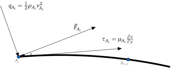
So let’s evaluate the above conditions. To study the impact of shape and size over fluid’s flow, let’s 98
consider two successive space domainsAi&Ai+1in the flow as shown in Figure 1[3].
τAi =µAi
∂v
∂y qA
i =
1 2ρAiv
2 Ai
θ
~ FA
i
Ai
Ai+1
Figure 1.Illustration of the resultant force vector on successive space domains in a stream line
99
1. Consider a infinitesimally small area as shown in Figure 1. Figure 1 illustrates that the the force 100
vectors due to dynamic pressure and shear stress of any pointAiin streamline which will interact with 101
adjacent pointsAi+1. On any given pointAiin the considered system where it has velocityv~i. Upon 102
interaction with other corresponding particles in the streamline, the velocity will change to∂ ~vi+v~i. 103
2. Thus there will be change in pressure normal toAi which is∂qAi+qAi. The force atAi is normal
104
vector to area. But the corresponding AreaAi+1will have an additional force vector on it with certain 105
angleθi. As per the equations (8), (9) (10) and (11), the force vector is an integral function over 106
considered infinitesimally small areaAi. For 2D flow it can be written as surface integral[8]So,F~A
iq
108
can be written as the resultant fluid dynamic force at a infinitesimally small area due to the dynamic 109
pressure of subjected motion of fluid atAi. F~A
iq is given quantitatively in equation (12).
110
~ FAiq =
‹
A
1 2ρAiv
2 Ai+
1 2ρAiq−1v
2
Ai−1cos(θr x y)
dA (12)
HeredAis infinitesimally small area between theAiand successive points.θr x yis the algebraic sum 111
of angles between resultant forces vectorsF~A
i andF~Ai+1along the streamline over the surface.
112
3. Similarly, the effect of shear stress distribution of resultant force atAican be given as: 113
~ FAiτ =
‹
A
µAi∂
vi
∂y +µAi−1
∂vi−1
∂y cos(θr x y)
dA (13)
Here, Equations (13) gives the effect of shear stress distribution over surface integral. As the second 114
components in the equations (12) to (13) are resultants of the succeeding elements and their effect is 115
dependent on the angleθr x y. 116
4. Therefore, the resultant force at a infinitesimally small areaAi can be written as sum equations (12) and (13).
~
FAi=
‹
A
1 2ρAiv
2 Ai+
1 2ρAi−1v
2
Ai−1cos(θr x y) +µAi
∂vAi
∂y +µAi−1
∂vAi−1
∂y cos(θr x y)
dA (14)
Equation (14) gives the resultant force at any given pointAi, which is the sum of the products of 117
the area with shear stress and dynamic pressure[6][8][3]. The resultant force of the preceding fluid 118
particles can be resolved on the given point with an angleθr and the resultant will have an effect on 119
succeedingAi+1. 120
Thus, equation (14) can be simplified as :
~ FA i = ‹ A 1 2ρAiv
2 Ai+µAi
∂vA
i
∂y +F~Ai−1cos(θr x y) dA (15) ~ FA i = ‹ A ~ FA
i+F~Ai−1cos(θr x y)
dA (16)
The effect ofF~A
i can be resolved in X-plane , Y-plane and Z-plane using trigonometric relations as
shown in equations (17) , (18) and (19). Here,θrx,θry andθrzare the angles at which force at any
pointAiacts on surrounding fluid particles along X-axis, Y-axis and Z-axis respectively.
Σn
0(θrx) =Σ
n osin−1
Ç |F~A
ix|
2− |V~ ix| |V~i x|
=0 (17)
Σn
0(θry) =Σ
n ocos−1
|V~i y| |F~Ai y|
=0 (18)
Σn
0(θrz) =Σ
n osin−1
Ç |F~A
iz|2− |V~iz|
|V~iz| =Σ n ocos−1
|V~iz| |F~A
iz|
=0 (19)
Depending upon the direction of flow and it’s magnitude the components ofθ can be represented as 121
sin, cos components in the OX,OY planes. Here,F~A
ix andF~Ai y are resolved components of the resultant
122
force in X-plane, Y-plane respectively. whereV~i xandV~i y are velocity vectors of stream lines in X-plane 123
and Y-plane respectively. 124
Equations (17),(18) and (19) shows the trigonometric relations between local velocity vector,θ and force. 125
along the stream line should be zero. Otherwise, streamline formation is disturbed leading to occurrence of 127
other phenomena such as vortex formation at trailing edge or down-wash. 128
So based on the above equations it can be explained that the formation of stream changes with the 129
degree of curvature of the body, its size, flow velocity, fluid density and dynamic viscosity of the fluid. As per 130
3rdand 4thpostulates the energy is transferred or transformed between two time intervals i.e. energy or 131
momentum lost by collided fluid particles and energy received by collided fluid particles from its surrounding 132
fluid particles. So there can be two time intervalst1−t2andt2−t3. 133
At a local areaAi the equation (16) can be written as:
~ FAi =
ˆ t3
t1 ‹
A ~
FAi+F~Ai−1cos(θr x y)
dA
d t (20)
~ FAi =
ˆ t2
t1 ‹
A ~
FAi+F~Ai−1cos(θr x y)
dA
d t+ ˆ t3
t2 ‹
A ~
FAi+F~Ai−1cos(θr x y)
dA
d t (21)
Equation (20) and (21) shows time integral of force at a local area (A) over the two successive events. 134
t1−t2is the time interval when fluid particle collide at the solid body’s surface and loose their momentum 135
and time intervalt2−t3is the period when collided particles receive momentum to continue their motion. 136
This is due to elasticity of the fluid and its tendency to attain thermodynamic equilibrium. Equation (20) 137
has both time integral and surface integral defining the force and angle at which the it is acting on the 138
corresponding fluid particle. The time integral defines the consecutive effects of the fluid particles motion 139
and surface integral corresponds to local changes on the surface. Where as theθ corresponds to the degree 140
of the curvature of the body which can be noted by the trigonometric relations shown in equations (17), 141
(18) and (19). 142
5. Discussions 143
5.1. Flow over a linear body 144
Consider a flat plate parallel to the free-stream with a smooth laminar flow as shown in Figure 2. In the 145
Figure 2 the flat plate ’f’ has a viscous laminar flow which is indicated by dotted stream lines. The thickness 146
and style of lines indicate viscosity at that particular point. The free body diagram of ’f’ shows force vectors 147
on upper surface and lower surface from leading edge to trailing edge. Here,F~uois the resultant force 148
vector on upper surface andF~l ois the resultant force vector on lower surface at leading edge. F~iuandF~il 149
are the resultant force at any given point in between leading edges and trailing edges respectively.θnis the 150
algebraic sum of all the respective angles ofF~A
i over the flat plate i.eθnu+θnl=θn. Here,Σ
nu
0uθ=θnuand 151
Σnl
0lθ =θnl.
q∞,ρ∞,v∞,a∞,µ∞
f ~
F0u F~iu F~nu
~
F0l F~il F~θnln=0
o f
Figure 2.Laminar flow over a flat-plate
152
So, at stagnation point if the body with stands these forces then substantial phenomenon are observed: 153
Thus, the resultant force of the stagnant fluid particles will be at an angle with respect to free-stream velocity. 154
The resulting force from stagnation point, which is acting over the surrounding fluid particles makes them 155
to flow around the upper surface and lower surface of the body will have change in theirθiuandθiland 156
in the velocity vectors of fluid particles moving on the upper surface and lower surface will continuously 158
have a increment in the angleθiand the magnitude of the resultant force|F~i|till the trailing edge. If the 159
sum ofθnu&θnlis equal to 0◦.[6]Then fluid particles flow in same direction as free-stream as long as the 160
magnitude ofF~nis not too high to deviate them from channeled stream line. Thus at low speed where the 161
magnitude of resultant aerodynamic force at trailing edgeRnis not too high and upper and lower surface 162
from stagnation point have same length and symmetric shape the flow remains laminar and smooth. As 163
this is a straight body, the fluid particles will have tangents for free-stream at the leading edges and trailing 164
edges of the body and change inθ is very minimal. Thus stream lines formed around the flat plate are 165
nearly parallel to it’s surface.So, from Figure 2 it can be stated that for a straight line body which is parallel 166
to the free-stream velocity vector(v∞~ )there won’t be much change inθi as long as the velocity is not too 167
high to disrupt the streamlines formed. 168
But as the velocity and length of body increases, we observe that the flow separation and turbulence 169
phenomenon posterior to the trailing edge. Even for a thick plate with considerable frontal area under 170
stagnation, we observe this phenomenon at low speeds. Because at higher velocity of the free stream and 171
large length of body, more energy is lost at stagnation point and subsequent fluid particles gain energy 172
and becomes turbulent as the resultant forces increases continuously and thus flow separation occurs as 173
the magnitude of the force at that particular point of separation is too high|F~i|to detach the fluid from 174
streamline. Thus fluid particles detach causing irreversible loss of the flow (turbulence) from the stream 175
line if they have enough energy to deviate from their respective streamlines as shown in Figure 3[3]. 176
Similar phenomenon can be observed in flat plates with angle of attack. As more area is opposing the 177
motion of the fluid particles at the area of stagnation is higher and the induced angle of attack contributes 178
to change in the direction of fluid particles as the force is already acting at an angle.[8]Like wise higher 179
velocity of free-stream tends to increase magnitude of resultant force closer to stagnation point. This leads 180
to stall velocity and stalling angle. 181
Based on Reynold’s number we can say that the dynamic viscosity (µ) is inversely proportional to 182
the turbulence on the surface of the body[8][5][2].The distance from stagnation point(l), velocity(~v) and 183
number of fluids particles available to receive momentum and transfer (ρ) are directly proportional to 184
turbulence on the body’s surface.[9]Therefore, based on historical data we can say that as long as Re<2300
Figure 3.Flow on a flat plate showing boundary layers of laminar and turbulent flows
185
at any point on the streamline of the flow will be laminar. Here,lin the equation (6.1) must be understood 186
Re= ρvl µ
Re<2, 300 l aminar f l ow 2, 300<Re<4, 000 t r ansi t ional f l ow
Re>4, 000 tur bul ent f l ow
(22)
Based on the conditions specified on can evaluate the nature of flow at any given point on the stream. 188
Here,lshould be considered from point of stagnation to the point of consideration on the streamline even if 189
it is posterior to the trailing edge. As it is already well known that the transfer of momentum is a continuum 190
effect in the flow. So, the fluid particles will retain the momentum even after passing away from the body 191
and thus they will tend to flow in turbulent nature posterior to the trailing edge. 192
Similarly a square or rectangular body will undergo above phenomenon and these can be analyzed 193
using fromulae and assumptions mentioned above. But it will have a larger area subjected to stagnation 194
and which will result in larger magnitude of resultant force|F~|. Thus the fluid particles closer to stagnation 195
point will have higher energy. This will contribute to earlier flow transition and flow separation compared 196
to a flat plate or a streamlined body like an airfoil. 197
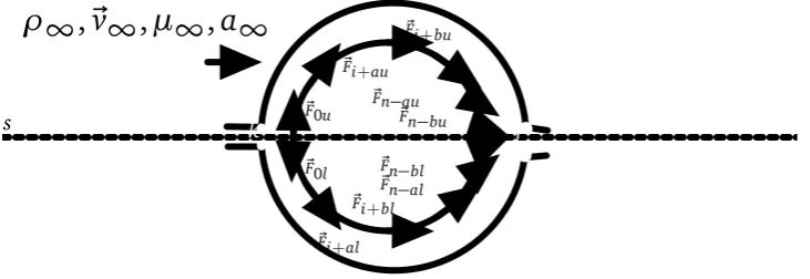
5.2. Flow over a curvilinear body 198
Consider a body with circular cross-section as shown in Figure 4. It will have a tangents all around 199
the body, unlike flat plate. So fluid particles will have continuous change inθalong their streamline. This 200
is due to the change in the body shape of the body. However as the body is symmetric, the magnitude of 201
the resultant force on the upper surface and magnitude of the resultant force on the lower will be equal i.e. 202
|F~iu|=|F~il|.[6][8]Similarly,θiu=θil. As discussed in equation (10) and (11), the line integral of angleθ 203
around a curved, symmetric body will be zero. So, under low Reynold’s number the flow will not experience 204
any separation and turbulence. However, the change inθis also continuum depending on the shape of the 205
body[2]. If the change is too significant and sufficient enough for the fluid particles to skip from their stream 206
line with considerable magnitude in the resultant force at a certain point, then flow separation will occur. In 207
this way a symmetric flow separation is occurred when the line of symmetry and free stream vectors are 208
co-linear. This is because the fluid particles will have opposing forces due to the path they traveled and 209
magnitude of the resultant force at the trailing will be high.[6]As fluid particles of same mass and velocity 210
collide which each other they will cause turbulence.
~
F0u
~
F0l
~
Fi+al
~
Fi+bl
~
Fn−al
~
Fn−bl
~
Fi+au
~
Fi+bu
~
Fn−au
~
Fn−bu
ρ
∞
,
~
v
∞
,
µ
∞
,
a
∞
j k
s
Figure 4.Flow over a circular cross-section body
211
Now consider a symmetric airfoil which has it’s line of symmetric or chord at zero incidence with the 212
free stream. It will not have any vertical force components or simply lift co-efficient is zero(CL=0). But it 213
will have a coefficient of drag or horizontal force componentCD0. This is because the vector of resultant 214
force and its direction is in the same direction as the free-stream. Many phenomena like flow separation, 215
But when the angle of attack is increased, more area is subjected to stagnation compared to flat plate and 217
curved body will have smooth change inθ. Thus symmetric airfoils will have higher performance compared 218
to flat plate at an incidence angle. 219
Flow over an asymmetric body such as cambered airfoils can be explained in the following way. The 220
asymmetric body will have unequal areas on its upper surface and lower causing flow on both surfaces to 221
have differentF~i andθi. Where force on one side is greater than other side and the angleθon one side of 222
the body is greater than the other side, the resultant forces will be have more magnitude towards one plane 223
even at zero incidence. Thus, camber airfoils will have a lift coefficient (Cl>0) even whenα=0. However, 224
they will have an effect called down wash. In cambered airfoils the line integrals ofθon both upper surface 225
and lower surface are not equal. As the length or area of the upper surface is higher than lower surface 226
with higher degree of curvature, It will haveθu, which is greater thanθl. Thus stream lines at trailing edge 227
seems little offset with free-stream. However, this effect is negligible, and the angle of down-wash is nearly 228
∼3◦t o5◦(based on historical data of aerfoils). 229
6. Conclusion 230
We enough know that the specified thickness of the body effects by progressively increasing Reynold’s 231
number due to more stagnation and energizing the fluid particles.[8]The length of the body will equally 232
contribute by contributing to the change in the magnitude of the resultant force at each consecutive point.[6] 233
These can be expressed using equations given in this article. Curvature of the body effects the streamline 234
by contributing to the change in the angleθ of resultant force at consecutive points from leading edge 235
to the trailing edge. Thus this article mathematically confirms these facts and explains the phenomena 236
such as stalling and effects of camber. With the above mathematical model formation of streamline, flow 237
separation and flow transition can be explained for a given body’s shape, size and flow parameters for a two 238
dimensional flow. 239
With FEM this mathematical model can help to estimate flow over a body i.e. to predict the formation 240
of streamline and changes along the streamline with respect to the free-stream velocity, dynamic viscosity 241
and body’s shape and size. This model can also be used to reduce the iterations in a design process especially 242
while performing itinerary shaping and sizing of a body in fluid dynamic system or components with open 243
circuit flow. In designing hydrofoils and airfoils, this model can have a significant impact in terms of shaping 244
and sizing compared to conventional methods. In traditional methods of designing streamlined body, where 245
a horizontal tear like body or circle is assumed with arbitrary dimensions (sometimes dimensions based on 246
historical data) and iterated to acquire desired performance. Later, designed models are tested by mostly 247
with scaled models. For a physical scaled model both Reynold’s number (Re) and Mach number (M) can’t be 248
same as its prototype. Thus, based on flow regime either one of them are not prioritized e.g for high speeds 249
mach number is more important the Re where as for low speeds Re tends to dominate experiment setup. 250
Unlike that, this method can start with a arbitrary dimension at the first preliminary phase and consequently 251
changing the shape at each successive interval or topological surface can deliver a faster design process with 252
less experimentation. In designing a streamlined body the mathematical model presented here presents a 253
lucid and quantitative parameters to design as this formulated model particularly identifies with effects of 254
shape and size of the body. Future scope of work involves developing a CFD(computational fluid dynamic) 255
solver based on the mathematical model prominently mentioned in this article. To objectively evaluate CFD 256
solver and mathematical model using experimental methods. 257
When we implement principles of classical mechanics, the mathematical model is unrealistic and 258
estimated values will have a significant deviation with respect to the real-time phenomenon. Though 259
solid body’s shape and size remain constant over the large duration, fluid particles from being static to 260
ionization (under high speeds) will go under various changes that even defies many laws in classical 261
mechanics. Moreover, it is required to extent the current model for a three dimensional flow which can be 262
accommodate not just a laminar flow. A further investigation is required how well this model is applicable 263
Funding:This research received no external funding
265
Acknowledgments:I thank Prof. Veeranjaneylu K, MLR Institute of Technology for improvising mathematical model
266
to be more realistic by suggesting proper assumptions, and Mr.Pavan Kumar B, Asst. Design Engg., AST Aersystems
267
Pvt. Ltd. for comments that greatly improved the manuscript quality and readability. I am immensely grateful for both
268
of them for their comments on earlier versions of the manuscript, although any errors in this article are my own and
269
should not tarnish the reputations of these persons.
270
Conflicts of Interest:“The authors declare no conflict of interest.”
271
Nomenclature
α Angle of incidence
∆~v Change in velocity vector of the fluid particles
∆T Change in the Temperature µ Dynamic viscosity of the fluid ρ Denisty of the fluid
θ F~∠v~∞-angle between the resultant force due to fluid flow and free stream velocity θrx Angle of resolved force component along
X-axis
θry Angle of resolved force component along
Y-axis
θrz Angle of resolved force component along
Z-axis
θr x y Angle between two succesive points or space domains along the streamline
~
Fx Horozontal component of Force ~
Fy Vertical component of Force ~
F Resultant force due to the fluid motion ~
v Velocity of the fluid Ar e f Reference Area CD Co-efficient of Drag CL Co-efficient of lift CF Co-efficent of force
l length
A Effective area
a Acceleration of the fluid M Mach number
m Mass of the fluid Re Reynold’s number t time interval
Subscript
∞ Parameters of free-stream velocity
L E Leading Edge
T E Trailing Edge
Ai Local parameters such asρ,µ,~Fand~vthe area (A) Aiq Local dynamic pressure on the area (A)
i Local parameters or derivatives on the streamline
ix Components of local parameters or derivatives on the streamline in the x-direction or parallel to free-stream
iu,0u,nu Components of local parameters or derivatives on the upper surface of the body
il,0ul,nl Components of local parameters or derivatives on the lower surface of the body
l o Lower surface of the body
uo Upper surface of the body
t1−t2 Time period between collision and momentum lost
t2−t3 Time between fluid particles stagnation and movement
272
References 273
1. Fifty years of boundary-layer theory and experiment. National Advisory Committee for Aeronautics; Washington,
274
DC, United Stateshttps://ntrs.nasa.gov/archive/nasa/casi.ntrs.nasa.gov/20150019333.pdf. Mar 18, 1955.
275
2. For McGraw-Hill Concise Encyclopedia of Physics:. center of pressure. (n.d.) mcgraw-hill concise encyclopedia of
276
physics. https://encyclopedia2.thefreedictionary.com/center+of+pressure, 2002. [Online; Retrieved March 2
277
2019].
278
3. Texas A and M University. Fluid mechanics - lecture notes - chapters 1-14,academic year 2014-15. Fluid
279
Mechanics-Lecture noteshttps://www.studocu.com/en-au/document/texas-am-university/fluid-mechanics/
280
lecture-notes/fluid-mechanics-lecture-notes-chapters-1-14/422911/view.
281
4. L J Clancy. Aerodynamics. 1975.
5. Mohamad Hafiz Ghani, Sarah , P X Khaleeda, C W Lim, and Phoa . Design and development of air flow sensor,
283
drag and lift force sensor and pressure sensor for air flow bench part 3. DESIGN AND DEVELOPMENT OF AIR 284
FLOW SENSOR, DRAG AND LIFT FORCE SENSOR AND PRESSURE SENSOR FOR AIR FLOW BENCH, 01 2016.
285
6. L M. HOSKINS. Theoretical mechanics; an elementary text-book, 1900.
286
7. John D Anderson Jr. Fundamentals of Aerodynamics. 2014.
287
8. G. Biswas S. K. Som. Fluid mechanics nptel(lecture notes on introductory fluid mechanics course). NPTEL-IIT
288
Kharagpur & IIT Kanpurhttps://archive.org/details/FluidMechanicsNPTEL/page/n9. Accessed: 2009.
289
9. Arnold Sommerfeld. "ein beitrag zur hydrodynamischen erkläerung der turbulenten flüssigkeitsbewegüngen (a
290
contribution to hydrodynamic explanation of turbulent fluid motions)". International Congress of Mathematicians,
291
1908. Pgs:116–124.
292
10. Andrea Ianiro Stefano Discetti.Experimental Aerodynamics. 03-2017.
293
11. Wikipedia contributors. Newton’s laws of motion — Wikipedia, the free encyclopedia. https://en.wikipedia.org/ 294
w/index.php?title=Newton%27s_laws_of_motion&oldid=886801669, 2019. [Online; accessed 2-April-2019].