An 1-D Integrated Hydro-Mechanical Model to Unravel Different Hydrological Triggering Processes of Debris Flows
Theo W.J. van Ascha,b , Bin Yub , Wei Hub
a. Faculty of Geosciences, Utrecht University, P.O. Box 80115, 3508 TC, Utrecht, the Netherlands.
b. State Key Laboratory of Geohazard Prevention and Geoenvironment Protection, Chengdu University of Technology, Chengdu, Sichuan, 610059, P.R. China;
[email protected] [email protected]
corresponding author : Th.W.J. van Asch Nachtegaalstraat 6 4116 BP Buren The Netherlands Tel: 00 31 344 571449 [email protected]
An 1-D integrated hydro-mechanical model to analyze different hydrological triggering processes of debris flows
Abstract
Many studies, which try to analyze the meteorological threshold conditions for debris flows
ignore the type of initiation. This paper focuses on the differences in hydrological triggering
processes of debris flows in channel beds of the source areas. The different triggering processes
were studied in the laboratory and by model simulation on the field scale. The laboratory
experiments were carried out in a flume, 8 m long and a width of 0.3 m. An integrated
hydro-mechanical model was developed, describing Hortonian and Saturation overland flow, through
flow, maximum sediment transport and failure of bed material. The model was tested on the
processes observed in the flume. The flume experiments show a sequence of hydrological
processes triggering debris flows, namely erosion and transport by intensive overland flow and
by infiltrating water causing failure of channel bed material. Model simulations carried out on a
schematic hypothetical source area of a catchment show that the type and sequence of these
triggering processes are determined by slope angle and the hydraulic conductivity of the bed
material. It was also clearly demonstrated that the type of initiation process and the geometrical
and hydro-mechanical parameters may have a great influence on rainfall intensity-duration
threshold curves, indicating the start of debris flows.
Key words: triggering of debris flows; overland flow; infiltration; laboratory experiments;
1 Introduction
A debris flow is the most dangerous type of mass movement because depending on the rheology
and topography it can reach a very high speed and large run-out distance. Important study
aspects are the mechanism and boundary condition of the initiation process of a debris flow,
because it determines the meteorological threshold conditions and further evolution and it will
provide clues for future mitigation strategies [1].
One can make different classifications of initiation mechanisms based on different viewpoints [1]
It was among others [2-3], who stressed the importance of the infiltration capacity of the soil as a
key factor for either the development of shallow landslides or surficial erosion and transport of
material by overland flow that might create different types of flow like mass movements. We
will use this hydrological classification principal in this paper and make a primary distinction
between overland flow driven and infiltrating driven initiation mechanisms. Effective overland
flow driven triggering processes are mainly concentrated in channels where high water
discharges, severe erosion and transport lead to high solid concentrations generating debris flows
[4-9]. Material is supplied to these debris flows by detachment and transport of the bed material
but also through lateral erosion of the channel bed. The channel can be partly or totally blocked
by landslide dams. High run off discharges eroding these landslide dams can also lead to
initiation and rapid grow of debris flows ([10-12]. Landslide damming can also be initiated by
rapid incision of the channel bed destabilizing the side walls [13]. With infiltrating driven
triggering mechanisms, shallow landslides are generated, which may or may not transform into
debris flows. This failure mechanism by infiltrating water can occur in channel beds filled with
flows [15-18]. The transformation of a failed mass into a debris flow is rather complex and
depends on various hydro-mechanical processes related to pore pressure development and supply
of abundant overland flow water further mobilizing the failed mass ([19-23].
Several authors analyzed partly or more completely the role of hydro-mechanical and
morphometric factors controlling the type of initiation of debris flows. Berti [24] analyzed the
hydrological factors for the generation of debris flows in typical source areas in the Italian Alps
by modelling channel overland in the channel bed from a source area as a response to rainfall
impulses. Kean [25] proposed an integrated hydro-geotechnical dynamic model to describe
sediment transport by overland flow and consequent mass failure transforming into debris flow
surges. Hu [26] highlighted the initial soil moisture and thus infiltration capacity as a controlling
factor on the type of initiation: wet soils created surficial erosion and incision, bank failure,
damming and debris flow development and for dry soils landslide failure and debris flows. [1]
Zhuang focused more on the slope gradient as a controlling factor for different types of initiation.
Their flume studies revealed that at gentler slope gradients around 100 ± 20 , incision and bank
failure is dominant creating channel damming and dam failure inducing debris flows. At
intermediate slopes around 150 ± 30 erosion of bed material occur at high discharges. The high
sediment transport capacity with high sediment concentrations is sufficient to create debris
flows. At steep slopes around 210± 40 bed failure by infiltrating overland flow water with debris
flow formation is the most dominant process.
Meteorological thresholds for the initiation of debris flows are closely related to the process of
initiation. In many studies about these meteorological thresholds, no clear distinction was made
morphometric and geological factors was made in most cases using statistical techniques
[28-30].
One can conclude that important triggering mechanisms occur in the channel of debris flow
gullies by overland flow in the source area. The first aim of this paper is to analyze with an
integrated 1-D hydro-mechanical model, the boundary conditions (hydraulic conductivity and
slope gradient) for the type and sequence of hydrological triggering mechanisms and thus mode
of debris flow initiation.
The second aim of this paper is to use this model to analyze in a physical way the effect of the
most important morphometric and hydro-mechanical factors on the meteorological threshold for
two types of initiation processes of debris flows namely overland flow and bed failure.
2 Description of the Flume experiments
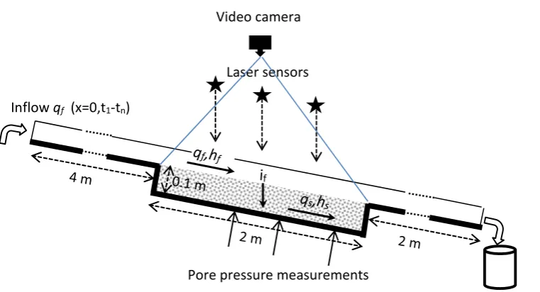
A flume was designed to simulate in a 1D frame work the initiation of debris flows by overland
flow and through flow (Figure 1). The flume has a length of 8 m and a width of 0.3 m. The
material simulating the channel bed with a thickness of 0.1 m and a width of 0.3 m is positioned
at a distance of 4 m from the top of the flume and has a length of 2 m. The material was brought
into the flume in layers of about 2 cm and was slightly compacted (dry density see Table1).
There is an outflow at a distance of 2 m from the lower end of the channel bed (Figure 1). The
water is entered at the upper end of the flume with a discharge, which can be controlled
Figure 1: Design of the flume test. For explanation of the parameters see text
Particle size class
Friction (o)
Density kNm-3
Hydraulic
conductivity (m s-1) D30 (mm) D50 (mm) D90 (mm)
Coarse 34.6 15.4 4.91E-03 9 11 18
Medium 33.7 16.3 3.28E-03 4 6 16
Fine 29.2 19.5 0.54E-03 0.7 1.6 8
Table I. Hydro-mechanical characteristics of three types of bed material, used in the flume tests. Friction means friction angle of the material in degrees. D30 means that 30% of the sample has a
lower diameter than what is indicated in the column (etc).
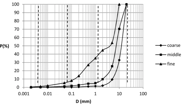
water from an upstream area. Three types of material were used in the experiments with different
grain size distributions (Figure 2). We could vary the slope angle of the flume between 140 and
200. The initial moisture content of the flume material was more or less dry. The initial moisture
Inflow qf (x=0,t1-tn)
Discharge measurements Pore pressure measurements
content is important for the infiltration capacity but since we used in the laboratory a large influx
of water from above into coarse bed material, we ignored the effect of the Sorpetivity (related to
the initial moisture content) on the infiltration capacity of the bed material.
Figure 2: Cumulative grain size distribution of the three bed materials, used in the flume tests
The friction of the three materials was measured with the conventional direct shear apparatus
[31] The hydraulic conductivity was measured with a constant-head permeameter. The hydraulic
conductivity of saturated cylindrical soil samples of the three grainsizes was measured with a
constant head gradient between the upper and lower end of the sample ([32]. Table I gives 0
10 20 30 40 50 60 70 80 90 100
0.001 0.01 0.1 1 10 100
P(%)
D (mm)
coarse
middle
further information about the friction, hydraulic conductivity and gradient of the materials used
for the experiments.
Pore pressure was measured at three places (Figure 1) at the bottom of the flume. The pore
pressure sensors, type :YP4049, were produced by Yom Technology Company. The measuring
range of pore pressure is from -100kPa to 100kPa.
Laser sensors (ZLDS100 ZSY Group; resolution 0.03 % FS) at three points with a spacing of 0.5
m (Figure 1) were used to monitor topographical heights, especially with the aim to monitor
abrupt changes in relief due to bed failure.
In addition video-recordings were performed (Figure 1) to follow the sequence of processes in
the course of the experiments. During the process of overland flow erosion, samples were taken
six times for more or less steady state conditions at the outlet of the Flume (Figure 1). The
discharge of water with sediments was collected in baskets during 5 seconds. The sediments
were sieved, dried and weighted to measure the concentration of the fluid.
An integrated model for surface and sub surface flow, sediment transport and bed slope stability
was developed to describe the processes in the flume, which was used later to analyze the
sequence of different initiation processes at the field scale.
3 1D integrated model for debris flow initiation in upstream channels
First we have to simulate the hydrological part of the triggering mechanism of debris flows. For
that we need the mass balance equation for overland (Eq.(1a)) and through flow (Eq.(1b)) ,
which is given by :
+ = (1b)
where qf is overland flow discharge per unit width (m3m-1s-1); qs is subsurface discharge per unit
width (m3m-1s-1); hfis thickness of overland flow (m); hs (m) is thickness of subsurface flow, x
(m) is distance along the slope t is the time (s) and B1-2 are terms (m s-1) describing the inflow
or outflow of water from the flow system, which is defined as follows:
= 0 − ( )− ( ) (2a)
= (2b)
where r (m s-1) describes the external input of rain into and if(m s-1) the outflow of water by
infiltration out of the overland flow system (Eq. (2a)) (see also Figure 1). When there is no
supply of rain, like in our flume experiments: r=0. In the case of subsurface flow if in Eq.(2b) is
considered now as an inflow term of the subsurface flow system. If hf/t is larger than the
infiltration capacity Ks (m s-1) of the bed material the latter one is the limiting factor. Therefore
the infiltration term if of Eq. (2)is the minimum (min) value of the infiltration capacity Ks (m s-1)
and the current water depth (hf), which can infiltrate in one time step t into the bed material:
:
= min ( , ℎ /∆ ) (3)
We introduce here a general momentum equation for the water flow processes [33]:
ℎ = (4b)
For turbulent overland flow the parameters fand f in Eq.(4a) can be defined as follows :
= .
.
and = 0.6 (5)
where n is Manning’s n and S0 the slope gradient of the bed material.
For subsurface flow we can write according to Darcy’s law:
= sin ℎ → ℎ = (6)
where qs is the amount of subsurface flow water per unit width (m3m-1s-1); is slope angle
(degrees) and hs is the height of the flowing water component in the soil matrix (m). By
comparing Eq.(6) with the general momentum Eq. (4b) we can define the parameters
sand s for subsurface flow:
= and = 1 (7)
A combination of the mass balance Eq.(1) with Eq.(4) delivers an expression for overland flow
or subsurface flow discharge (qf,qs) [33]:
+ ( , ) = (8a)
The 1D model is implemented in a fixed Eulerian frame where the variation in water flow
variables is described at fixed coordinate points at a distance x along the slope as a function of
time step t. A numerical solution for Eq.(8) is given by [33]:
=
∆
∆ ∆
∆ ∆
(9)
where qx, and should be read as qf,s f,s and f,s respectively.
To simulate the initiation of debris flows by mass failure we used the equation for the infinite
slope equilibrium model [31], which is the trigger for failure:
=( ) (10a)
= ℎ cos (10b)
where F is the safety factor; failure occurs when F=1; s and w are the saturated bulk density of
the material and water respectively; is friction angle of the material; z and hsare the thickness
of the soil and the height of the groundwater layer respectively hs can be solved with Eq. (9) and
Eq.(6) respectively.
The overall stability of the bed material expressed with the safety factor (F) for the infinite slope
model is calculated as an average of the safety factor of the different nodes. The inflow of water
into the flume is coming from upstream and therefore the pore pressure gradient is decreasing
average approach of the safety factor over the length of the sample in the flume seems a
reasonable approximation of the overall safety factor.
For estimating the transport capacity on steep slopes Rickenmann [34-35] proposed a bedload
transport equation based on a shear stress approach, where discharge, bed slope gradient and
material grading are used as parameters to characterize flow hydraulics.
For steeper slopes, in the range of 0.03<S<0.2 (1.7o-11.3o) Rickenmann [34] performed a
regression analysis with the steep flume data on bed load transport obtained at ETH Zurich that
resulted in the equation:
=( .) . . − (11)
where D90 and D30 are grain sizes at which 90% and 30% respectively by weight of the material
are finer; dsis the mass density of the solids and S is the slope gradient and qc is the critical flow
discharge for bed load entrainment. The experimental slopes were in the range of 0.03>S>0.20.
(1.70-11.30) and the D90 of the material ranged between 0.9>and2 cm and D30 between 0,06 and
1 cm with inflow rates of 10-30 l/s In the paragraph below we will calibrate Eq.(11) for the
steeper slopes in our flumes
4 Results of the flume tests
4.1 Initial observations during the flume tests.
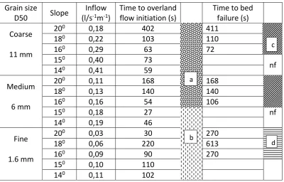
During the flume tests with the three bed materials under different slope angles, observation
flow initiation, time to overland flow initiation and bed failure, surficial erosion phenomena,
critical slope angles for bed failure and type of bed failure (Table II).
Grain size
D50 Slope
Inflow (l/s-1m-1)
Time to overland flow initiation (s)
Time to bed failure (s)
Coarse
11 mm
200 0,18 402 411
180 0,22 103 110
160 0,29 63 72
150 0,40 73
nf
140 0,41 59
Medium
6 mm
200 0,11 168 168
180 0,13 140 140
160 0,16 54 106
150 0,18 27 nf
140 0,19 46
Fine
1.6 mm
200 0,03 30 270
180 0,06 220 613
160 0,09 90 270
150 0,10 110
140 0,11 102
Table II. Observed time to overland flow and bed failure, overland flow type and failure mode in flume experiments for three types of bed material and for different bed slope angles: a)
Saturation overland flow; b) Hortonian overlandflow; c) slow continuous bed failure; d) rapid failure; nf: no failure.
In slope hydrology two types of overland flow can be distinguished: Saturation overland flow
and Hortonian overland flow [32]. These two types could be distinguished during the different
flume experiments (Table II). Saturation overland flow was characterized, after complete
saturation of the soil, by a more or less spatially randomly ponding of water at the soil surface,
while Hortonian overland flow, which occurs when the rainfall intensity or supply of overland
flow water is larger than the infiltration capacity of the soil, showed a more concentrated
continuous flow all over the flume According to these visual indicators we could establish a
a
b
boundary between Saturation overland flow and Hortonian overland flow, which in our flume
tests was found in the medium grain size materials at a slope gradient of 160 (Table II). This
could be verified with our model simulation (see below paragraph 4.2). For courser materials (Ks
values of 4.19E-03 and 3.28E-03 m s-1 ) and higher slope angles (> 160 ) the time to Saturation
overland flow is immediately followed by failure or with a small delay until 9 seconds. Also one
can clearly observe that the time to Saturation overland flow (and thus failure) is decreasing with
decreasing slope angle (Table II) .
Hortonian overland flow [32].was initiated in most cases on the finer sediments, which is
ascribed to the lower infiltration capacity (Ks = 0.54E-03 m s-1). Bed failure in this case occurred
a certain time after the start of the Hortonian overland flow with a time lag ranging between 35
and 160 seconds (Table II), because in this case, due to the lower percolation rate it takes time to
bring the groundwater in the bed material to a critical failure level.
Bed failure initiation is controlled by the bed gradient and the internal friction of the material and
occurred in our experiments on slopes of approximately 16 degrees and higher. At lower slope
angles no bed failure occurred (nf in Table II) and sediment delivery occurred only by overland
flow erosion
The medium and course materials show bed failure characterized by slow movements over the
total depth combined with fast surficial entrainment of grains by saturated overland flow.
Movement of bed material is slow and continuous or sometimes intermittent showing a surging
pattern (Table II). Instead of the slow and more flow like movements observed for the medium
and coarse sediments, failure of the fine sediments occurred suddenly with a very rapid surge of
Sediment transport by overland flow on these steep slopes reached volumetric concentrations
between 0.46 and 0.64 which is characteristic for debris flows
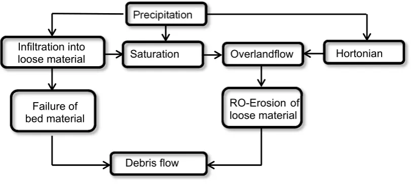
Fig 3 schematic diagram showing the different initiation processes of debris flows in channels
We can conclude on the basis of these observations that the flume tests carried out with the three
materials revealed three types of processes, which created debris flows on these range of slopes
gradients namely debris flow Initiation by Hortonian Overland flow Erosion (RhE-I), Saturation
Overland flow Erosion (RsE-I) and by Bed Failure (BF-I). The occurrence and sequence of these
processes seems to be controlled by slope gradient and hydraulic conductivity of the bed
sediment. Figure 3 gives a schematic overview of these process types.
4.2. Modelling the flume test processes
The next step was to model some of the processes in the flume. We used a number of process
indicators from the flume experiments to validate the outcomes of our model. These are : Precipitation
Overlandflow
RO-Erosion of loose material
Debris flow Infiltration into
loose material
Failure of bed material
Saturation or Hortonian overland flow, time to overland flow, maximum pore pressure, time to
bed failure and solid concentration by overland flow erosion. Hortonian overland flow and the
time to Hortonian overland flow in the model is declared when surface water hfreaches the lower
end of the bed material while the bed material is still not satured (hs < Zs) .Saturation overland
flow and the time towards it, is declared when hs = Zs over the entire bed. Pore pressure is
calculated each time step according to Eq (10b). The discharge of hf + hs is reported each time
step at the end of the flume. Bed failure is declared as said before when the average Safety factor
F over the bed length reaches the value of 1
For the flume simulations the distance between the nodes (x) was 0.1 m and the time interval
(t) was 0.2 seconds.
Figure 4 Observed and calculated time to Saturation overland flow (black symbols) and Hortonian overland flow (open symbols)
Figure 4 shows the relation between observed and calculated time to overland flow for the
different flume tests. There is a moderate 1:1 correlation between observed and predicted time to
0 20 40 60 80 100 120 140 160 180
0 50 100 150 200
time
to
ove
rla
nd
flo
w
ob
ser
ved
(sec)
Time to overland flow Calculated (sec)
coarse
medium
overland flow for the medium and coarse sediments and for the fine sediments, showing
Hortonian overland flow, there is no correlation at all. However the model was able to predict the
type of overland flow according to what was observed during the flume tests (see Table II).
Despite the malfunctioning of some pore pressure sensors we were able to make an 1:1
comparison between the average maximum measured pore pressure for the three sensors (Figure
1) and the average calculated maximum pore pressure (Figure 5).
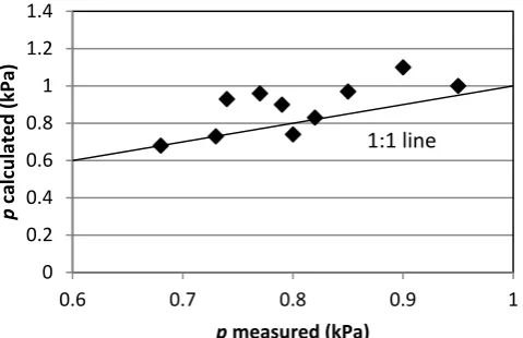
Fig 5 Maximum pore pressure measured during flume tests in relation to calculated pore pressures.
The Figure shows that in many cases there is a slight overestimation of the calculated pore
pressure. Time series of measured pore pressure of the three sensors compared to modelled
temporal pore pressure development showed thatin most cases the onset towards maximum pore
pressure for the three sensors is more irregular compared to the calculated development of the
pore pressures (Figure 6) . This can be ascribed to the heterogeneity of the sediment or (and) the
imperfect response of the sensors
0 0.2 0.4 0.6 0.8 1 1.2 1.4
0.6 0.7 0.8 0.9 1
p
calcul
ated
(kPa
)
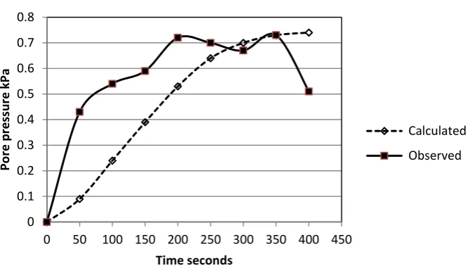
Fig 6 Example of the rise in pore pressure (measured /calculated) due to infiltration of run-on water in the bed material (Test:Medium grain size /200)
In relation to pore pressure development we compared the time to failure for the different test
runs on the different materials. Since the time towards average maximum calculated and
measured pore pressure coincided more or less, one would expect also corresponding calculated
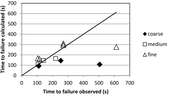
and measured failure times. Table II and Figure 7 show that the match between observed and
calculated failure time is reasonable except for two outliers (coarse-200 ;fine-180). Further we
can observe that the calculated time to failure is underestimated for the coarse material and
overestimated for practically all the tests on the medium and fine materials. The deviations
between calculated and observed values must be ascribed to heterogeneity of the material,
deviating friction values, and incorrect assessment of the overall safety factor
0 0.1 0.2 0.3 0.4 0.5 0.6 0.7 0.8
0 50 100 150 200 250 300 350 400 450
Po
re press
ure
kP
a
Time seconds
Calculated
Figure 7: Observed and calculated time of failure of bed material during the flume tests.
We calibrated also the parameters of the Rickenmann [35] equation, (Eq.11) on our flume tests,
which were carried out on slopes ranging between 0.25>S>0.36 (140-200), with grain sizes for
0.9>d90>2 and 0,05>d30>1 cm and with flow rates 0,5>qf>15 l s-1 m-1. Figure 8 shows the best
linear fit between qsolid/qf and(d90/d30)0.2S2, which delivered the following modified equation for
slopes between 140 and 200:
= 7.28 . (12a)
which gives for ds=2.6 :
=( . ) . . (12b)
0 100 200 300 400 500 600 700
0 100 200 300 400 500 600 700
Time
to
fail
ur
e
calculated
(s)
Time to failure observed (s)
coarse
medium
Figure.8. Calibration of Rickenmann’s bedload equation for steeper slopes in our flume tests between 14 and 20 degrees.
The calibration revealed that qc in Eq.(11) becomes zero or practical zero in Eq.(12). At slopes
larger than 150 the down slope component of the grain weight may reduce the critical shear stress
c which in our case obviously reduced to nearly zero
5. Sensitivity analyses at the field scale
5.1A schematic source area for sensitivity analyses at the field scale
To study the influence of terrain parameters and the hydro-mechanical parameters on debris flow
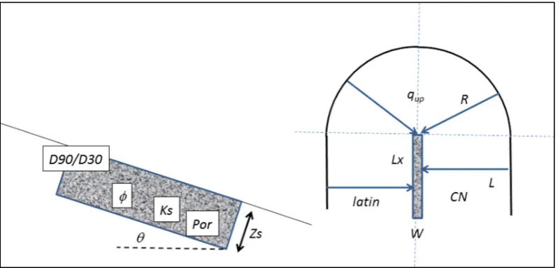
initiation a schematic source area of a catchment is proposed here. Figure 9 shows this schematic
source area, which is linked to an upstream channel filled with bed material receiving surface
water from the surrounding slopes to initiate a potential debris flow. This geomorphological
setting resembles more or less the source areas described among others by Coe [7] and Berti
[24]. The upstream area of our hypothetical catchment has a radius R. The channel is further
surrounded by lateral slopes with a length L. The length of the channel bed is Lx , the width W
y = 7.2866x R² = 0.832
0.4 0.6 0.8 1 1.2 1.4 1.6 1.8 2 2.2 2.4 2.6
0.04 0.06 0.08 0.1 0.12 0.14 0.16 0.18 0.2
qs/qf
and the slope angle is .The hydraulic conductivity of the bed material is Ks the porosity Por
and the friction angle . (Figure 9).
Figure 9: Morphometric and hydro-mechanical parameters, which were used for model simulations of debris flow initiation. For an explanation see Table 3 and text. D90/D30: 90% and 30% lower than grainsize D90 and D30 respectively :
friction angle; Ks: hydraulic conductivity; Por :porosity; Zs: depth of material; : slope angle, qup: water that flows into theupper end of the channel bed; R: radius of source area above the channel; Lx and W: length and width of the channel bed; L: length of lateral contributing slope; latin: lateral inflow of water to the channel; CN: curve number value for the soil hydrological and land use characteristics of the contributing slopes.
The sink term B in (1) and (8) is now adapted to the field scene and given by:
= 2 + − (13)
where latin (m s-1) is the lateral inflow of overland flow water from the slopes along the channel
Eq.(3)). The lateral inflow is calculated for these sensitivity analyses in a simple way, assuming
steady state conditions in the mass balance equation for overland flow:
= (14)
rcn (m/s) is calculated using the Curve Number method [36], L is the length of the lateral slope
and W the width of the channel (see Figure 9). In our simulations we selected overland flow
supplying slopes with soils with moderate to slow infiltration rates and a poor condition grass
cover, which corresponds to a Curve Number(CN) of about 80. The CN number, reflecting the
hydrological soil characteristics, land use and antecedent soil moisture conditions that we can
expect in high mountainous areas, was chosen arbitrarily and was kept constant in our
simulations. The overland flow water that flows into the upper end of the channel bed is given by
qup (m2 s-1) (Figure 9)
= . (15)
5.2The influence of the hydraulic conductivity (Ks) and slope () of the channel bed on
the type and sequence of hydrologic triggering processes for debris flows
In the flume we could observe the effect of slope angle and hydraulic conductivity on the type
and sequence of triggering processes which may lead to the initiation of debris flows. In this
paragraph we will investigate through model simulation the effect of these two factors on the
catchment scale. The values of the other factors used in our model simulations are shown in bold
Ks for RE-I 0.001-0.0025-0.005 m s-1 Lx 50-100-200 m
Ks for BF-I 0.001-0.01-0.1 ms-1 Por 0.4-0.3-0.2
Zs 2-4-6m R 250-350-450 m
28-32-36 L 250-350-450 m
16o-20-28o n bed 0.08
W 2-4-6-m
Table III. Default values (bold italic) and maximum and minimum values of input parameters for Overland flow Erosion (RE-I) and Bed Failure (BF-I) triggering debris flows. Ks: saturated hydraulic conductivity; Zs: thickness of bed material;friction angle of material; slope angle of channel bed; W and Lx :width and length of channel bed respectively; Por: available volumetric pore space; R radius of source area ; L: length of lateral slopes ; n: Manning’s n of bed material.
The data shown in Table IV are obtained from our modelling scenarios as explained in Paragraph
4.2. Table IV gives an overview of the range in Ks values (first row) and bed slope angles (first
column), which were used in our simulations to study the effect of these parameters on the
hydro-mechanical process development at the catchment scale. For these simulations two rain
scenarios were used with an intensity of 80 mm (Table IVa) and 40 mm per hour (Table IVb)
respectively. The Tables show domains with different shades of gray with various combinations
of hydro-mechanical triggering processes. In the white sections no debris flow initiation is
expected to develop in the source area because of a too low sediment concentration of the
overland flow. Table IVa shows that in the domain 280-200 and Ks= 0.001-0.005 m s-1, the
debris flow is initiated in the first stage by Hortonian overland flow erosion (RhE-I). The
overland flow discharge reaches a steady state after a certain relatively short time. During the
steady state groundwater will rise by infiltration of run-on water until failure of the bed material,
see a dramatic drop in discharge between slopes with Ks =0.001 and 0.005. The last value
reaches a significant boundary which determines whether or not debris flow can be initiated by
Hortonian overland flow transport.
80 mm Ks 0.001 m s-1 0.005 m s-1 0.01 m s-1 0.1 m s-1
Slope degrees Initiat proc. Time min. Dischar l s m-1
Time min.
Dischar l s m-1
Time min.
Dischar l s m-1
Time min.
Dischar l s m-1
Concent l l-1
28 RhE-I BF-I
1.0 5.4
912 1.3
1.7
139
2.4 3.0 0.47
24 RhE-I BF-I
1.0 8.4
783 1.3
2.3
119
2.8 3.1 0.39
20 RhE-I BF-I
1.1 11.2
683 1.4
2.9
104
3.1 3.1 0.30
16 RhE-I RsE-I
1.1 14.2 606 732 1.5 3.7 92
733 3.7 732 3.6 705 0.21
12 RhE-I RsE-I
1.2 14.8 550 666 1.5 3.9 83
665 3.8 664 3.6 646 0.13
a
40 mm Ks 0.001 m s-1 0.005 m s-1 0.01 m s-1 0.1 m s-1
Slope degrees Initiat proc. Time min. Dischar l s m-1
Time min.
Dischar l s m-1
Time min.
Dischar l s m-1
Time min.
Dischar l s m-1
Concent l l-1
28 RhE-I BF-I
1.5 5.8
162
7.2 7.9 8.0 0.47
24 RhE-I BF-I
1.6 8.8
139
7.8 8.2 8.3 0.39
20 RhE-I BF-I
1.7 11.7
121
8.5 8.5 8.4 0.30
16 RhE-I RsE-I
1.8 14.8
108
234 9.5 235 9.4 233 9.3 208 0.21
12 RhE-I RsE-I
1.9 15.0
98
214 9.6 213 9.5 212 9.2 170 0.13
b
Table IV. Time sequence of different initiation processes RhE-I and RsE-I,(erosion by Hortonian
and Saturation overland flow respectively) and BF-I (bed failure) in relation with hydraulic conductivity (Ks) and slope angle of bed material. Further are given the discharge (Discharg) and solid concentration (Concent) during RhE-I and RsE-I. Table 4a and 4b: simulated rain
It is confirmed by Table IVb with a lower rain input (40 mm) where at Ks ≥ 0.005, no initiation
by Hortonian overland flow is possible anymore.
Going back to Table IV-a: in the domain 160-120 and Ks= 0.001-0.005 ms-1 slope failure does
not occur. The debris flow is initiated by overland flow. First by Hortonian overland flow and
later when the groundwater has reached the surface by Saturation overland flow. Discharge is
relatively low when there is Hortonian overland flow, while obviously discharge dramatically
increases at Saturation overland flow. However due to the lower slope angles, the volumetric
sediment concentration is low (0.21 at 160 and 0.13 at 120, (Table IV-a last column ), which
means the flow changes from a hyper concentrated flow into a water flood with conventional
suspended load and bed load.
At higher conductivities in the domain Ks=0.01-0.1 m/s and 28o-20o, bed failure seems the
most dominant process (Table IVa). Due to the larger Ks values, infiltration into the bed is more
important than overland flow discharge. The bed material turns out to be partly saturated in the
upper part due to the larger upstream inflow, creating partly Saturation overland flow and
Hortonian overland flow. However within one minute after the run off discharge reached the
lower end of the bed, failure of the bed material occurred already. Therefore the contribution of
overland flow to the transport of debris by overland flow can be ignored.
In the domain Ks=0.01-0.1 m/s and lower slope gradients (16o-12o ) there is no slope failure
but only Saturation overland flow, (Table IVa ) with low sediment concentrations in most cases
not enough to call it a debris flow.
Table IV-b shows the simulation results with an intensity of 40 mm per hour. The domains with
a specific combination of hydro-mechanical triggers still exist. There is only a shift of the
IVa and b show a decrease in overland flow discharge and increase in time to bed failure with a
decreasing slope angle. Around 16 degrees the channel bed is stable but still steep enough to
have transport capacities with concentrations in the domain of a hyper concentrated flow. These
are induced by Hortonian and Saturation overland flow at lower Ks values and only Saturation
overland flow at higher Ks values. At lower slope angles (see slopes around 12 degrees)
sediment concentrations are too low to call it a debris flow. Table V gives a summary of the type
and sequence of initiation processes related to different Ks and slope angle values.
40mm Ks values 0.001 m s-1 0.005 ms-1 0.01 m s-1 0.05 m s-1 0.1 m s-1
Gradient Flow type Initiation process Initiation process
28o
Debris flow
t1:Hortonian overland flow
t2:Bed failure
t1: Bed failure 24o
20o
16o
Hyper
concentrated flow
t1:Hortonian overland flow
t2:Saturation overland flow
t1:Saturation overland flow
12o No debris
flow
t1:Hortonian overland flow
t2:Saturation overland flow
t1:Saturation overland flow
5.3. Factors influencing rain Intensity-Duration (I-D) threshold curves for different
initiation processes of debris flows
In the foregoing we revealed the influence of Ks and bed slope gradient on the sequence of two
main processes mechanisms involved in the initiation of debris flows. We want to investigate
here the effect of the other parameters (including Ks and slope gradient) on rainfall thresholds in
terms of Intensity Duration (I-D) curves for the triggering of debris flows by these two process
mechanism: initiation by Hortonian overlandflow (RhE-I) and bed failure (BF-I). As we have
seen in Table IV and V, debris flow initiation by Saturation overland flow (RsE-I) can only take
place around 16 degrees At lower slope angles sediment concentrations are too low to call it a
debris flow (Table IV). At higher slope angles we have bed failure before Saturation overland
flow can take place. Figure 10 shows the effect of different parameters on the I-D curves for
debris flows initiated by Hortonian overland flow. The intensity and duration value of a rain
event which creates overland flow that just reaches the end of the channel bed with a sediment
concentration of >0.2, is defined by us as a threshold rain event for debris flow initiation. The
intensity and duration values for a variety of different critical rain events were plotted in a graph
with on the y-axis the intensity and on x-as the duration. In this way an Intensity Duration (ID)
curve can be constructed. Table III gives an overview of the range of the different parameters
and the default values (in bold italic), which were used in the simulation and which give a
realistic representation of geometric and geotechnical parameters for source area conditions The
threshold curves for debris flow initiation by Hortonian overland flow are shown in Figure 10. In
this figure the threshold curves which are constructed, using the default values given in table III,
are depicted with open rectangular markers. They are equal in all the sub-figures. This enables
default curve. For each combination of selected parameters there is an ultimate minimum rain
intensity below which not enough overland flow and thus a debris flow can be initiated,
irrespective
Figure 10. I-D curves for debris flow initiation by Hortonian overland flow in relation to different geometrical and hydrological parameters. For the definition of parameters see Table III 0 20 40 60 80 100
0.5 1 1.5 2 2.5 3
In te ns ity ( m m /hr) Duration (min) Ks
Ks=0.0005 Ks=0.0010 Ks=0.0050 Ks=0.0025
0 20 40 60 80 100
0.5 1 1.5 2 2.5 3
Inten ity (m m /h r)
Duration ( min) 0 20 40 60 80 100
0.5 1 1.5 2 2.5 3
In te nity ( m m /h r)
Duration ( min) n
n=0.06 n=0.08 n=0.10
0 20 40 60 80 100
0.5 1 1.5 2 2.5 3
In te ni ty ( m m /hr )
Duration ( min) R&L
R&L=250 R&L=350 R&L=450
0 20 40 60 80 100
0.5 1 1.5 2 2.5 3
In ten it y (mm/ hr )
Duration ( min) Lx
Lx=50 Lx=100 Lx=200
0 20 40 60 80 100
0.5 1 1.5 2 2.5 3
In te nity ( m m /h r)
Duration ( min) W
W=2 W=4 W=6
a b
c
e f
the duration (D) of the rain event (see horizontal dotted lines). The simulations show that at
intensities below this critical dotted line the overland flow water never reach the lower end of the
bed due to a too high infiltration rate on its pathway compared to the supplied overland flow
water and finally bed failure will be the primary triggering process.
The most obvious selected parameter for overland flow initiation is the hydraulic conductivity Ks
Other parameters are related to geometry of the source area (see Figure 6) like length of the
lateral slopes along the channel (L ), radius of the upstream area of the channel (R) Length (Lx)
and width (W) of the channel bed , channel bed gradient ( and further Manning’s n of the bed
material.
For run off initiation by Hortonian overland flow we saw in the forgoing that this triggering
mechanism plays a dominant role for Ks values < 0.005 m s-1. Figure 10 a shows the influence of
the Ks value on the I-D threshold curves for run off erosion initiation (RhE-I). The range of Ks
values is chosen between 0.0005 and 0.005 m s-1 The Figure shows that for Ks values lower than
0.001 m s-1 there is nearly no effect of Ks on the position of the I-D curve but there is a
difference in the minimum intensity values (dotted lines) below which no debris flow can occur.
A slight difference can be observed for lower intensities (<60 mm hr-1)..Higher Ks values (>
0.001 m s-1) have a larger influence on the I-D curves. (Figure 10a)
The simulations show that the scale of the source area and lateral slopes (R&L), the length of the
river bed (Lx) and the width of the bed (W) have the largest effect on the position of the
threshold curve for the initiation of debris flow by Horton overland flow (Figure 10 b,d,f
respectively). The threshold curves are less sensible for the effect of the slope gradient and
Figure 11. I-D curves for debris flow initiation by bed failure in relation to different geometrical and hydro-mechanical parameters. For the definition of parameters see Table III
0 20 40 60 80 100
0 5 10 15 20 25 30 35 40 45 50 55 60 65 70 75 80
In te n it y (mm/hr )
Duration ( min) Ks
Ks=0,001m/s Ks=0,01 ms-1 Ks=0,1 m/s
0 20 40 60 80 100
0 5 10 15 20 25 30 35 40 45 50 55 60 65 70 75 80
In te nity ( m m /h r)
Duration ( min) Por
Por=0.2 Por=0.3 Por=0.4
0 20 40 60 80 100
0 5 10 15 20 25 30 35 40 45 50 55 60 65 70 75 80
In te nity ( m m /h r)
Duration ( min) 0 20 40 60 80 100
0 5 10 15 20 25 30 35 40 45 50 55 60 65 70 75 80
In
te
nity
(
mm/hr)
Duration ( min) 0 20 40 60 80 100
0 5 10 15 20 25 30 35 40 45 50 55 60 65 70 75 80
Intenit y (m m /h r)
Duration ( min) R&L
R&L=250m R&L=350m R&L=450m
0 20 40 60 80 100
0 5 10 15 20 25 30 35 40 45 50 55 60 65 70 75 80
In te n ity ( m m /h r)
Duration ( min) Lx
Lx=50m Lx=100m Lx=200m
0 20 40 60 80 100
0 5 10 15 20 25 30 35 40 45 50 55 60 65 70 75 80
Intenit
y
(mm
/h
r)
Duration ( min) W
W=2m W=4m W=6m
0 20 40 60 80 100
0 5 10 15 20 25 30 35 40 45 50 55 60 65 70 75 80
In te ni ty ( mm/hr)
Duration ( min) Zs
Figure 11 shows the influence of the different geotechnical and geometrical factors on the
threshold values for the triggering of debris flows by bed failure. The range in Ks values for
which bed failure (BF-I) is the dominant process is chosen between 0.001 and 0.1 m s-1 with a
default value of 0.01 m s-1 The effect of the selected range in geometric values R&L ,Lx,W, ,
and Zs ( Figure 11 b,d,f,g,h respectively) seems to be more or less the same. Less effect have the
porosity Por of the bed material and the values (Figure 8 c,e respectively). No effect has the
hydraulic conductivity Ks (Figure 8a), which is related to the simplicity of the model describing
instantaneous downward percolation for these high permeable bed materials. Interesting is to see
that at lower Ks values (around 0.001 m s-1) and higher rain intensities the rate of groundwater
storage and therefore the critical duration for failure is nearly the same (Figure 8a).
Our I-D curves obtained by our simulations suggest that the duration range is strongly influenced
by the type of initiation. Debris flows initiated by Hortonian overland flow seems to be initiated
within several minutes while debris flow initiated by bed failure within one to two hours. I-D
curves find in the literature give threshold curves with a larger duration range of one to several
hours. The relative quick response to debris flow initiation can be explained by the large effect
we give in our simulations to the contributing slopes with sparse vegetation and low infiltration
rates, which in other areas may be minor due to vegetation, and consequently higher infiltration
rates and lower overland flow rates. The use of the curve number method also explains the quick
response to initiation; because it does not take into account the effect of the initial moisture
content with for dry soils gives larger infiltration rates and time to ponding in the first period of a
rain event. It also does not simulate the travel time towards the channel. The relative quick
response for channel bed failure initiation was also found by by Berti [24] dealing with nearly
Fig 12 Ultimate variation in I-D curves as a result of our sensitivity analyzes compared to the
maximum difference in I-D curves found world wide
Fig 12 compares two extreme I-D curves [38-39] and one between the two [37] obtained world-
wide with the two extreme curves produced in our simulation, The curves are displayed in a
log-log plot because of clarity The minimum curve in our simulation is related to the maximum
channel slope (280) and the maximum threshold curve is related to the largest length (Lx) of the
channel bed. Fig.12 shows that a simple variation of parameters for the initiation of debris flows
in channel beds, gives already a relative wide range in variation compared to the range in
threshold values for debris flows worldwide. The larger decline of our ID-curves compared to
some of the curves worldwide may be also subscribed to the important role of the contributing
slopes surrounding our hypothetical channel in the source area.
6. Discussion
This paper unraveled the effect of different hydro-mechanical processes on the initiation of
debris flows. It is focused on the initiation in channels and it gives a detailed insight in the
1 10 100
10 100
Intesit
y
( mm/hr)
Duration minutes
This paper (q)
This paper (Lx)
Innes (1983)
Chien-Yuan et al. (2005)
Caine (1980)
influence of different hydro-mechanical process mechanisms in the source area on the mode and
sequence of debris flow initiation. It shows how different morphometric and hydrological
factors, especially the hydrologic conductivity (Ks) and slope gradient ( determine the type of
these process mechanisms.
Our simulations suggest that the type of initiation and related factors have also a clear influence
on the values of the I-D curve as shown in Fig 10 and 11. These I-D curves, determined by our
two simulated process mechanisms, Hortonian overland flow and bed failure show a relative
quick response of debris flow initiation compared to wat is generally provided by the literature.
Our calculations were focused on the initiation of debris flows in the source area in channel beds
surrounded by slopes with scarce vegetation and rather impermeable soils. A quick response
(within one hour) was also observed by Berti [24] where, as in our simulations, debris flows
were initiated in the source area by the dominant effect of run-on water to the channel delivered
by a bare impermeable catchment upstream.
The assessment of rainfall threshold values for debris flow initiation are based in most cases on
statistical empirical approaches using large data sets without detailed knowledge of the different
triggering processes and its influencing factors [2, 29].
Our quantitative approach to analyze the threshold conditions for debris flow initiation gives a
more detailed insight in the effect of different parameters than the indicative parameters used in
statistical techniques. Apart from the fact that no distinction is made in the mechanism of
initiation, important morphometric characteristics, like channel width, slope length thickness of
bed material etc, are ignored in most cases. As a consequence the prediction of rainfall threshold
Further investigations must reveal the accuracy of both approaches to predict the initiation of
debris flows.
The CN value, which we used in the simulation of overland flow on the contributing slopes,
reflects in a lumped way the dynamic soil and land use characteristics. Especially the amount of
storage of water before the time to ponding and thus the estimate of the total overland flow
production of a rain event can be rather inaccurate especially for rain events of shorter durations.
The use of a more detailed infiltration model incorporating the effect of the initial moisture
content will give better prediction. However in this paper we did not unravel in detail the effect
of these soil and land use characteristics on threshold conditions for debris flow initiation but
uses a constant CN value as input for the run-on simulation to the channel bed. Initial moisture
conditions in the channel bed, which will affect the permeability and hence the boundary
conditions for initiation for overland flow initiated debris were not considered either in this
paper. The effect of the initial moisture content of the bed material is minor due to the large
amounts of influx of water and the relative coarse material in the channel bed.
In this paper we mentioned the transport capacity of overland flow as a limiting factor for the
initiation of debris flows. On slopes (<±16o ) sediment concentrations are too low (<0.2) to call it
a debris or hyper concentrated flow. For these lower channel gradients we did not consider the
effect of the delivery of extra material by side wall collapses and failure of landslide dams[1, 13],
which may lead downstream to a rapid loading of the fluid and an instantaneous transformation
into a debris flow
The initiation of debris flows by bed failure is also more complex since it depends on certain
boundary conditions related to pore pressure development at failure and a large amount of run
It is interesting to analyze the potential in development further downstream of debris flows
triggered by bed failure (BF-I) with high solid concentrations. On steeper slopes failure of the
bed material occurs under lower groundwater heights (hs) and therefore after failure much
additional overland flow water is needed to maintain the movement further down slope.
Important is also the mechanism of erosion and erosive power of both types of debris flows
further downstream in order to grow to a mature debris flow [6, 40-43].
7.Conclusions
Three types of hydro-mechanical processes were distinguished which can trigger debris flows in
channel beds of first order source area. These are erosion and transport by intensive Horton
overland flow (ROh-I), Saturation overland flow (ROs-I) and by infiltrating water causing failure
of channel bed material (BF-I). We were able to assess by means of a hydro-mechanical model
the boundary conditions for the mode of debris flow initiation. The hydraulic conductivity of the
bed sediments is an important factor controlling the type and sequence of processes triggering
debris flows. At lower Ks values Hortonian overland will be the first process to start debris flows
followed by bed failure or Saturation overland flow. At higher Ks values triggering by Hortonian
overland flow is not possible anymore in this relatively coarse bed material and triggering by bed
failure will be the dominant process if the slope gradient is steep enough (>160) . Therefore the
slope gradient of the channel bed is a second important factor controlling the type of
hydo-mechanical triggering. On gentler slopes which remain stable under saturated conditions,
Saturation overland flow might create debris flows if slope gradient is not too gentle and
therefore sediment concentration too low to call it a debris flow.
We further analyzed also the effect of different important morphometric and hydro-mechanical
failure respectively. With respect to overland flow triggering, the morphometric factors related to
the size of the source area and width and length of the channel bed have the largest influence on
position of the I-D curves. Meteorological thresholds for bed failure triggering are also sensitive
to morphometric parameters while the hydro mechanical parameters have relative less influence
on these threshold values.
References
[1]Zhuang, J.; Cui, P Peng J.; Hu, K.; Iqbal, J. Initiation process of debris flows on different
slopes due to surface flow and trigger-specific strategies for mitigating post-earthquake in
old Beichuan County, China. Environmetal. Earth Sciences. 201368, 1391–1403; DOI 10.1007/s12665-012-1837-2.
[2]Cuomo, S.; Della Sala, M. Rainfall-induced infiltration, runoff and failure in steep unsaturated
shallow soil deposits. Eng. Geol. 2013, 162, 118–127.
[3]Cuomo, S.; Della Sala, M.; Novita, A. Physically based modelling of soil erosion induced by
rainfall in small mountain basins. Geomorph. 2015, 243, 106-115.
[4] Berti, M.; Genevois, R.; Simoni, S.; Tecca P.R. Field observations of a debris flow event in
the Dolomites. Geomorph. 1999, 29, 265–274.
[5]Armanini, A.; Gregoretti C. Triggering of debris flow by overland flow: a comparison
between theoretical and experimental results. Proceedings 2nd International Conference on
Debris flow Hazards Mitigation, Taipei, Taiwan;Wiezczorek, Naeser Eds. 2000, 117–124. [6]Takahashi, T.. Initiation and flow of various types of debris flow. Proceedings 2nd
International Conference on Debris Flow Hazards Mitigation: Mechanics, Prediction and
[7] Coe, J.A.; Kinner, D.A.; Godt, J.W.. Initiation conditions for debris flows generated by
runoff at Chalk Cliffs, central Colorado. Geomorph. 2008, 96, 270–297.
[8] Yu, B. Research on the prediction of debris flows triggered in channels. Natural Hazards,
2011,58, 391-406; DOI 10.1007/s11069-010-9673-8.
[9] Van Asch, Th.W.J.; Tang, C.; Zhu, J; Alkema. D. An integrated model to assess critical
rainfall thresholds for the critical run-out distances of debris flows. Nat. Hazards,2014 70 (1), 299–311.
[10] Tang, C.; Rengers, N.; Van Asch, T.W.J.; Yang, Y.H.; Wang, G.F. Triggering conditions
and depositional characteristics of a disastrous debris-flow event in Zhouqu city, Gansu
Province, northwestern China. Nat. Hazards Earth Syst. Sci.,2011.,11, 2903–2912. [11] Cui, P.; Zhou, G.G.D.; Zhu, X.H.; Zhang, J.Q.. Scale amplification of natural debris flows
caused by cascading landslide dam failures. Geomorph. 2013,182 173–189.
[12] Zhou, G.G.D.; Cui, P.; Chen, H.Y.; Zhu, X.H.; Tang J.B.; Sun, Q.C. Experimental study on
cascading landslide dam failures by upstream flows. Landslides2013, 10 (5), 633-643. [13] Hu, W.; Xu, Q.; van Asch, T.W.J.; Zhu, X.; Xu, Q.Q.. Flume tests to study the initiation of
huge debris flows after the Wenchuan earthquake in S-WChina. Eng. Geol.,2015a, 182,
121–129.
[14] Cannon, S.H.; Kirkham, R.M.; Parise, M. Wildfire-related debris flow initiation processes,
Storm King Mountain, Colorado. Geomorph. 2001,39, 171–188.
[15] Hungr, O.; Evans, S.G.; Bovis, M.J.; Hutchinson, J.N. A review of the classification of
[16] Malet, J-P.; Laigle, D.; Remaître, A.; Maquaire, O. Triggering conditions and mobility of
debris flows associated to complex earthflows. Geomorph.,2005, 66, 215–235.
[17] Cascini, L.; Cuomo, S.; Della Sala, M.Spatial and temporal occurrence of rainfall induced
shallow landslides of flow type: a case of Sarno-Quindici, Italy.Geomorph., 2011126(1–2), 148–158.
[18] Zhang, S.; Zhang, L.M.; Peng, M.; Zhang, L.L.; Zhao, H.F.; Chen, H.X. Assessment of risks
of loose landslide deposits formed by the 2008 Wenchuan earthquake. Nat. Hazards and
Earth Syst. Sci2012. 12, 1381–1392; DOI:10.5194/nhess-12-1381-2012
[19] Iverson, R.M.; Reid, M.E.; LaHusen, R.G. Debris flow mobilization from landslides. Ann.
Rev. of Earth Plan. Sci.1997,25, 85–138.
[20] Fuchu, D.; Lee,C.F.; Sijing, W. Analysis of rainstorm-induced slide-debris flows on natural
terrain of Lantau Island, Hong Kong. Eng. Geol., 1999, 51, 279–290.
[21] Gabet, E.J.; Mudd, S.M. The mobilization of debris flows from shallow landslides.
Geomorph., 2006,74, 207–218.
[22] Van Asch, Th.W.J.; Malet, J-P. Flow-type failures in fine-grained soils: an important aspect
in landslide hazard analysis. Nat, Hazards and Earth Syst Sci2009, 9, 1703–1711. [23] Hu, W.; Donga, X.J.; Xua, Q.; Wang G.H.; Van Asch, T.W.J.; Hicher, P.Y.. Initiation
processes for overland flow generated debris flows in theWenchuan earthquake area of
China. Geomorph., 2016,253, 468–47.
24] Berti, M.; Simoni, A.. Experimental evidences and numerical modelling of debris flow
[25] Kean, J. W.; McCoy, S.W.; Tucker, G.E.; Staley, D.M.; Coe J.A. Runoff-generated debris
flows: Observations and modeling of surge initiation, magnitude, and frequency. J.
Geophys. Res. Earth Surf.,2013, 118, 2190–2207.;DOI:10.1002/jgrf.20148.
26] Hu, W.; Xu, Q.; Wang, G.H.; van Asch, T.W.J.; Hicher, P.Y. Sensitivity of the initiation of
debris flow to initial soil moisture. Landslides,2015,12, 1139–1145; DOI: 10.1007/s10346-014-0529-2.
[27] Liu, C.; Dong, J.; Peng, Y.; Huang, H. Effects of strong ground motion on the susceptibility
of gully type debris flows. Eng. Geol. 2009. 104(3–4), 241–253.
[28] Chang, T.C.; Chien, Y.H. The application of genetic algorithm in debris flow prediction.
Environmental Geology., 2007 53, 339–347.
[29] Tiranti,D.; Bonetto, S.; Mandrone, G. Quantitative basin characterization to refine
debris-flow triggering criteria and processes: an example from the Italian Western Alps. Landslides
2008, 5, 45–57.
[30] Yu, B.; Li,L.; Wu, Y.; Chu, S. A formation model for debris flows in the Chenyulan River
Watershed, Taiwan. Natural Hazards2013, 68, 745-762; DOI: 10.1007/s11069-013-0646-6. [31] Smith. G.N.;Smith, I.G.N. Elements of Soil Mechanics 7th ed.;Blackwell Science Ltd
Oxford, UK, 1988; 494 pp.; ISBN0-632-04126-9.
[32] Hendriks M.R. Introduction to physical Hydrology, 1st ed. Oxford University press: Oxford
,UK, 2010; 331 pp.; ISBN 978-0-19-929684-2.
[33] Chow, V.T.; Maidment, D.R.; Mays, L.W.. Applied hydrology. McGraw-Hill Book
company: New York, USA, 1988,572 pp. ISBN 0-07-010810-2.
[34]Rickenmann, D.. Hyperconcentrated flow and sediment transport at steep slopes. Journal of
[35] Rickenmann, D. Comparison of bed load transport in torrents and gravel bed streams. Water
Resources Research 2001,37(2), 3295-3305.
[36] USDA-SCS. National Engineering Handbook, Section 4:Hydrology 1985, USDA-SCS. Washington D.C,USA.
[37] Caine, N.; The rainfall intensity duration control of shallow landslides and debris flows.
Geogr. Ann. A Phys. Geogr.1980,62(1/2), 23–27.
[38 Innes, J.L. Debris flows. Progr. Phys. Geogr.1983, 7(4,) 469-501; DOI:.org/10.1177/030913338300700401
39] Chien-Yuan.;C.;Tien-Chien, C.; Fan-Chieh,Y.;Wen-Hui,Y.;Chun-Chieh,T. Rainfall duration
and debris-flow initiated studies for real-time monitoring. Environ. Geol.2005, 47, pp. 715-724, DOI: 10.1007/s00254-004-1203-0
[40] McDougall, S.; Hungr, O. Dynamic modelling of entrainment in rapid landslides. Can.
Geotech. J. 2005, 42, 1437–1448.
[41] Medina, V.; Hürlimann. M.; Bateman, A.. Application of FLATModel, a 2D finite volume
code, to debris flows in the northeastern part of the Iberian Peninsula. Landslides2008,5, 127–142.
[42] Iverson, R.M,.;Reid, M.E.; Logan, M.; LaHausen, R.G.; Godt, J.W.; Griswold, J.P. Positive
feedback and momentum growth during debris-flow entrainment of wet bed sediment.
Nature Geosciences. 2011. 4, 116–121.
[43] Quan Luna, B.; Remaître, A.; Van Asch, Th.W.J.; Malet, J-P,; Van Westen, C.J. Analysis of
debris flow behavior with a one dimensional run-out model incorporating entrainment. Eng.