Statistical modeling and optimization of the
EDM parameters on WC-6%Co composite
through a hybrid response surface
methodology-desirability function approach
S. Assarzadeh and M. Ghoreishi
Department of Mechanical Engineering, K. N. Toosi University of Technology, P.O. Box: 19395-1999, Tehran, Iran
Corresponding author e-mail: [email protected], Tel: +98-21-84063210, Fax: +98-21-88677274 Abstract
This paper presents an integrated approach to the process modeling and multi-objective optimization of electro-discharge machining (EDM) parameters on cobalt-bonded tungsten carbide composite (Tungsten Carbide-Cobalt alloy: WC/6%Co, Iso grade: K10) based on response surface methodology (RSM) coupled with desirability function (DF) technique. Four independent parameters, viz., discharge current (A), pulse on-time (B), duty cycle (C), and average gap voltage (D) were selected as the input variables to evaluate the process performance in terms of material removal rate (MRR), tool wear rate (TWR), and surface roughness (Ra). Face-centered central (FCC) composite design has been employed to plan and analyze the experiments. A comprehensive analysis of variance (ANOVA) at different significance levels of 1%, 5%, and 7% were done to fully identify the most influential parameters, and the adequacy of all fitted second order regression models were checked. To fully understand the characteristic machinability behavior under different EDM conditions, main effects analysis along with parametric analysis of the impacts of combinatory different important interactive factors were then performed scrutinizing 3D surface and 2D contour plots. It has mainly been revealed that all the responses are affected by the rate and extent of discharge energy but in a controversial manner. The MRR increases by either enhancing electrical discharge density or rising sparking frequency. Low TWRs can essentially be established by a combination of low current levels with prolonged pulse on-times or longer pulse on-times with smaller duty cycles. Less rough surfaces are achievable via a blend of either low current intensity with shorter pulse on-time or low current level with higher gap voltage. Finally, a multi-objective optimization technique based on the use of desirability function (DF) concept was then applied to the response equations to simultaneously find optimal combinations of input parameters capable of producing the highest possible amount of MRR and lowest amounts of TWR and Ra within the considered input process domain. The obtained predicted optimal results were then interpreted and verified experimentally to compute confirmation errors. The values of relative validation errors, all being found to be quite satisfactory (about 11% at the worst case), proves the efficacy and reliability of suggested approach.
Key words: Analysis of variance (ANOVA), Desirability function (DF), Electro-discharge machining (EDM), Face centered central (FCC) composite design, Multi- objective optimization, Process modeling, Response surface methodology (RSM), Tungsten carbide cobalt composite (WC-Co).
1. Introduction
Electro-discharge machining (EDM) is an electro-thermal erosion process where material is removed by a successive trend of controlled rapid and repetitive discrete electrical discharges (sparks), produced by a DC pulse generator, taking place between tool and work piece electrodes submerged in a liquid dielectric medium [1-3]. It is the most popular non-traditional machining method capable of eroding every electrically conductive material with an electrical resistivity threshold value of the order between 100-300 Ωcm as the only limiting factor to support sparking [4]. Since thermo-electric energy is used instead of mechanical forces; hence, the work-based metallurgical and micro structural properties such as strength, hardness, toughness, etc have no barrier against its applicability. For decades, the process has gained considerably popular applications in machining various engineering materials, especially high-strength, temperature-resistant (HSTR) alloys (Inconel, Titanium, Beryllium alloys) [5-7], hard composites (metal matrix composites, nano-composites) [8, 9], conductive ceramics [4, 10], etc. in miscellaneous industries, with the additional versatility as being a very promising approach towards micro- as well as nano-machining technologies [11-13].
[14]. Its acutely high hardness and strength, superior wear and corrosion resistance over a wide range of temperature has frustrated conventional machining processes of efficiently being utilized in shaping such a material. Though, the EDM process has now been recognized and justified as the best and perhaps the only proficient machining candidate for cutting and shaping tungsten carbides, however, the process is not an easy going task [15]. Furthermore, unlike steel, often chosen as a general option for work piece material in EDM applications, it has been postulated that the behavior of ceramic composites, such as WC-Co, can be rather different in response to various parameters under the EDM process [4, 10, 15] which still needs to be further studied as cited by Garg et al [8]. The main difficulty in EDMing WC-Co originates from its non-homogeneous structure, the differences between melting and evaporation points of the two constituent phases present in its micro-structure, i.e., WC and Co grains which may cause non-uniformity in erosion as well as process instability [15]. The melting and vaporization points of WC are about 28000C and 60000C, respectively, and those for Co are about 13200C and 27000C, both at normal atmospheric pressure [15]. Hence, during the EDM, the cobalt matrix first starts being removed from the surface by melting and evaporation mechanisms due to sparking. This early selective decomposition of WC-Co structure will lead to dislodging coarse WC grains into the gap space increasing the risk for process instability as a result of high debris accumulation and pollution inside gap region. Moreover, there is a noticeable difference in thermal expansion coefficients of WC and Co, the latter possessing a much higher one (14×10-6 1/0C for Co as compared to 5×10⁻⁶ 1/0C for WC) [10, 15]. The discrepancy is responsible for developing high thermal tension stresses during re-solidification and quenching, exceeding the fracture strength of the material in the crater, and thus, causing abundance of cracks on the surface layer. For these reasons, the electro discharge machining of WC-Co composite is regarded as a challenging task imposing more difficulties compared to EDMing different kinds of hardened steels commonly studied in research articles.
1.1 Literature review
Lee and Li [16] studied the effects of EDM parameters on surface characteristics of a kind of tungsten carbide. They have concluded that MRR and surface roughness of the work piece are directly proportional to the discharge current intensity. In their another research [17], a comprehensive qualitative analysis of surface integrity of ISO standard P-grade tungsten carbide under EDM conditions with peak current and pulse on-time variations was done. Miscellaneous aspects of surface integrity like micro-cracks, recast layer formation and surface roughness were studied. It was pointed out that the quality of work surface is a function of two main parameters, peak current and pulse duration, both of which are settings of the power supply. In a more quantitative manner, Puertas et al. [18] applied a 23 full factorial design with four center points to provide protection against curvature in model building of EDMing 94WC-6Co ceramic composite solely under finishing stages. Though, different significant main and interaction effects between input parameters were identified using ANOVA and their variations over selected responses were studied, however, neither a definite input settings nor a numerical value of machining factors were obtained as optimum values since no suitable optimization strategy was then tried. The same previous authors [19] conducted a comparative study of the die sinking EDM of three different conductive ceramics, viz. WC-Co, B4C, and SiSiC in terms of MRR, Ra, and TWR as response
technological variables using the same aforementioned DOE plan under only finishing regime using low discharge energy levels. They have indicated that the investigated ceramic materials showed different behaviors in response to the alterations of input factors except for MRR function which manifested the same trend for all the work piece materials.
lowest roughness amongst other tool electrodes. Banerjee et al. [25] applied face-centered central composite design to collect experimental data and RSM to model and analyze the processing parameters involved in EDMing WC-TiC-TaC/NbC-Co cemented carbide. They have found that sufficient superheating of work piece material and subsurface boiling are essential for efficient material removal. Liu et al. [26] carried out a set of experiments on EDM drilling of WC-Co based on rotatable central composite design to evaluate and analyze the edge disintegration created around holes’ rims. Major significant parameters were identified using ANOVA and by developing second order response equation, optimal input settings resulting in the minimum amount of damage around holes were obtained. Finally and most recently, Puertas and Luis [27] studied the behavior of two highly practical conductive ceramics in industry, B4C and WC-Co, under different die sinking EDM
conditions. Though, practical recommendations on how to adjust process settings to acquire low surface roughness, low electrode wear, and high MRR were suggested independently within input process domain, however, neither a precise optimization strategy nor a particular numerical parametric setting was then proposed to trade off between those conflicting objective responses as they were treated autonomously from each other without considering their mutual interdependencies.
1.2 Structure and merits of the adopted approach
Based on whatsoever stated before in opening the basic subject and reviewing related past researches, the major motivation of the present study is to fully understand and characterize the machinability measures of WC-6%Co in a more quantitatively systematic way in order to identify the right effects of various interfering parameters, alone as well as in combination with other factors, influencing process responses. In this regard, face-centered central composite design (CCD) of experiments has been adopted to plan the experiments. Adequately sufficient second order response equations, i.e. MRR, TWR, and Ra, are developed based on RSM using multiple linear regression analysis along with the ANOVA in which all significant main, quadratic, and two-way interactive effects are present pre documented by Student t-tests. Subsequently, the process responses are optimized to yield the best operating parameters combinations satisfying the highest possible MRR, lowest TWR and Ra simultaneously in a compromise manner using aggregated desirability function idea. The foremost merits of current research can be mentioned as follow:
a) By far, to the best of authors’ knowledge acquired through extensively reviewing related literature, the
simultaneous numerical optimization of MRR, Ra, and TWR in the EDM of tungsten carbide has not
yet been implemented. In the bibliography consulted, still there is lack of practical knowledge on EDMing WC-Co as scant technological tables useful for EDM researchers can be found compared to those widespreadly available for miscellaneous kinds of hardened steels [8].
b) Despite the fact that several experimental works have been directed toward studying EDMing WC-Co from different aspects [15], however, in their best cases, they have been either ended at the point of merely developing respective responses without any attempt to enlightening exact numerical optimal conditions [21, 24] or obtaining optimal conditions without bearing in mind the interdependency of all three main outputs (MRR, TWR, and Ra) at the same time as one of which has often been omitted [22, 23, 27]. In addition, no effort has yet been made into applying desirability function method aiming to optimize the EDM parameters of WC-6%Co composite, all at once in a compromise manner.
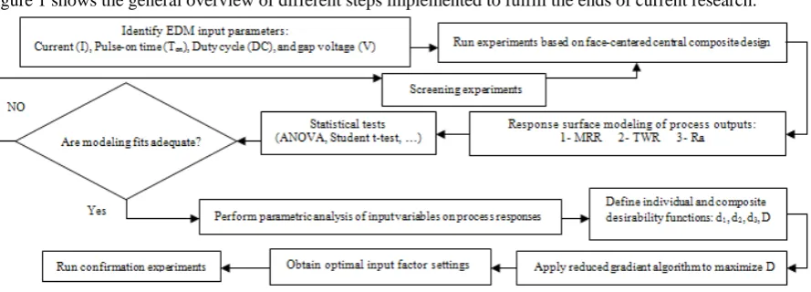
Figure 1 shows the general overview of different steps implemented to fulfill the ends of current research.
2. Experimental details
2.1 Machine tool, tool electrode, work piece and dielectric materials
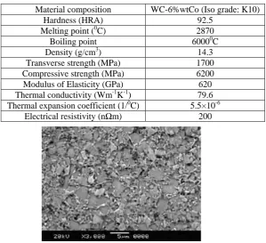
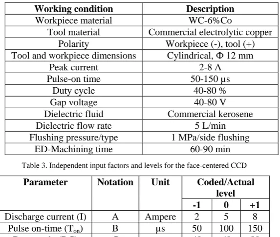
Azarakhsh ZNC spark erosion machine, model number 204 has been used to run the experiments. Equipped with an iso-frequency pulse generator, it can produce pulse-on times in the range 2µs-1000µs and provide maximum discharge current up to 75 A. Tungsten carbide cobalt composite, type WMG10, manufactured by Wolframcarb company, Italy, available in cylindrical form (Ф12mm×300 mm) has been selected as work piece material. A Charmilles Robofil 290 WEDM machine has been used to cut the blanks into 10 mm height to collect experimental samples. The selected WC-Co composite, produced via powder metallurgy, having about 94%wt WC and 6%wt Co as nominal chemical composition, is of a fine grain type and mainly used in fabricating drawing dies, woodworking tools as well as cutting tools for non-ferrous metals. Table 1 lists the relevant work piece material properties while Figure 2 illustrates its SEM micrograph.
As for the tool electrode material, electrolytic copper rods with the same diameter as work piece were used. The physical and mechanical properties are a density of 8.9 g/cm3, thermal conductivity 226 W/mK, electrical resistivity 9 µΩcm, melting point 1083 0C, and hardness about 100 HB. Copper has the additional advantageous as being easily available, stable in quality and cheap compared to other applicable metals. Thereupon, the EDM experiments were all conducted in planing mode in which both the tool and work piece bottom surfaces were ground prior to experimentation to remove any possible machining marks or irregularities assuring consistent initial gap width and flushing action. Moreover, commercial grade kerosene ejected as impulse side flushing through a nozzle was used as dielectric liquid carrying out machining debris from gap zone. Also, tool and work piece electrode polarity were assigned as positive and negative, respectively, as this status can make tool wear minimum along with stable sparking [10].
2.2 Machining parameters, design of experiments, and measurements
Four controllable input variables, namely, discharge current (A: Amp), pulse-on time (B: µs), duty cycle (C: %), and average gap (reference) voltage (D: Volt) have been selected as the predominant factors based on the EDM machine operating characteristics and consulting respective bibliography. These factors are the most relevant electrical-based parameters governing the discharge energy which is the most responsible item in EDM process efficiency [1, 2].
The discharge current, here, is the maximum value of discharge current intensity, that is, the peak intensity provided by the machine DC generator according to the magnitude of resistants placed on its electrical circuit. Pulse on-time (Ton) is the amount of time per cycle in microseconds during which the electric current is allowed
to flow. Duty cycle is defined as the ratio of pulse on-time to the total cycle time (pulse period) expressed in percentage [28], i.e.,
Table 1. Work piece thermo-physical and mechanical properties
Material composition WC-6%wtCo (Iso grade: K10)
Hardness (HRA) 92.5
Melting point (0C) 2870
Boiling point 60000C
Density (g/cm3) 14.3
Transverse strength (MPa) 1700
Compressive strength (MPa) 6200
Modulus of Elasticity (GPa) 620
Thermal conductivity (Wm-1K-1) 79.6
Thermal expansion coefficient (1/0C) 5.5×10⁻⁶
Electrical resistivity (nΩm) 200
: % 100 (1)
It is evident from the above definition that the duty cycle and pulse-off time have a reciprocal relation, i.e., at a constant value of pulse on-time, increasing duty cycle results in lower pulse-off time and vice versa. Finally, the gap or reference voltage is the average discharge voltage that the EDM machine servo system tries to maintain during the whole period of erosion and is a measure of spark energy as higher gap voltage results in stronger electrical discharge.
Face-centered central composite design (CCD) [29-31], a popular variant of central composite design of experiments, has been employed to plan the experiments. It is a kind of second order design class which uses three levels for each parameter and can efficiently handle linear, quadratic as well as interaction terms in process modeling. Generally, to collect enough data establishing a suitable second order regression response equation for a process involving k variables, the following three sets of design points are needed:
(a) nf = 2k factorial design or corner points
(b) na = 2k axial or star points, and
(c) nc center points, which are usually repeated several times to obtain a good estimation of experimental
pure error.
Then, the total number of experiments would be:
N = nf + na + nc = 2k+2k + nc (2)
The location of axial points in a response surface central composite design with respect to the center point (origin) is determined by alpha (α) value. The choice of α depends to a great extent on the domain of operation and interest [29]. In face-centered central composite design, α = 1, meaning that a three-level design space, coded as -1, 0, and 1 corresponding to low, medium, and high parameter level, respectively. To specify the actual levels of each input variable, at first, a number of preliminary tests were conducted as one-factor-at-a-time (OFAT) approach to determine the most stable combination of parameter settings over the operability region of EDM machine [32]. Table 2 summarizes the relevant machining conditions and fixed parameters whereas Table 3 lists the preferred input controllable parameters along with their ranges in both coded and actual format.
Table 2. The EDM conditions
Working condition Description
Workpiece material WC-6%Co
Tool material Commercial electrolytic copper Polarity Workpiece (-), tool (+) Tool and workpiece dimensions Cylindrical, Ф 12 mm
Peak current 2-8 A
Pulse-on time 50-150 µs
Duty cycle 40-80 %
Gap voltage 40-80 V
Dielectric fluid Commercial kerosene
Dielectric flow rate 5 L/min
Flushing pressure/type 1 MPa/side flushing
ED-Machining time 60-90 min
Table 3. Independent input factors and levels for the face-centered CCD
Parameter Notation Unit Coded/Actual level
-1 0 +1 Discharge current (I) A Ampere 2 5 8
Pulse on-time (Ton) B µs 50 100 150
Duty cycle (DC) C - 40 60 80
Gap voltage (V) D Volt 40 60 80
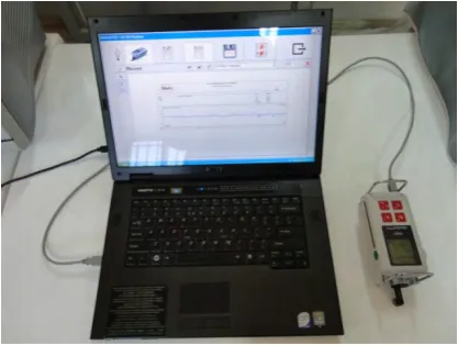
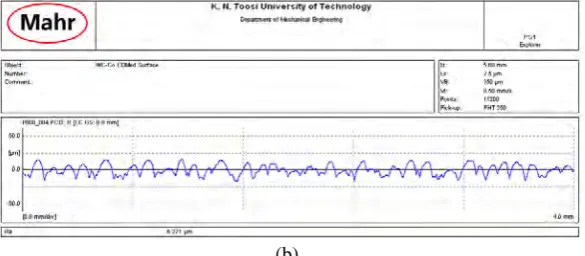
longer times were needed to get a reasonable idea about the MRR as the removal efficiency for cemented carbides are very small compared to steels due to its extremely hardness and wear resistance [25, 32]. So, the time allocated to each trial was at least an hour and much longer times were considered for runs with lower discharge currents. Characterization of each work piece surface condition was conducted in term of arithmetic mean deviations of roughness profile from the central line along the measurement path. Mahr-PS1 unit, a portable stylus type profilemeter made-up by Mahr Company, Germany, was used for roughness assessments. Before measuring surface roughness, each machined sample was cleaned in acetone liquid and dried with cold air blower. To achieve validity and accuracy, each Ra measurement was repeated two times along two different directions, as there is no specific pattern for spark distribution over the work area. The average of the two replications was then assigned as the roughness value for each treatment combination. Figure 3 shows a picture of the measuring device. In all cases, a cutoff length of 0.8 mm and an evaluation length of 4 mm (5×0.8 mm) were adjusted on the unit according to ISO 4287/1.
Figure 3. Mahr-PS1 surface roughness measuring unit
By repeating seven center points, the total numbers of conducted experiments for k = 4 was 24+2(4) + 7 = 31, and are shown in Table 4 along with the corresponding process responses. Figure 4(a) and (b) depicts two typical roughness profiles equivalent to two extreme cases, Exp. No. 19 and Exp. No. 16 in Table 4, processed by the MarSurf PS1 Explorer software, version 1.00-10, having the lowest and highest value of Ra, respectively. The linear relationship between coded and actual values, in Tables 3 and 4 is as follow:
Discharge current: A = [I-(Imax+Imin)/2]/ (Imax-Imin)/2
Pulse on-time: B = [Ton-(Tonmax+Tonmin)/2]/ (Tonmax-Tonmin)/2
Duty cycle: C = [DC-(DCmax+DCmin)/2]/ (DCmax-DCmin)/2
Gap voltage: D = [V-(Vmax+Vmin)/2]/ (Vmax-Vmin)/2
where A, B, C, and D are the coded values of variables I, Ton, DC, and V, respectively, Imax, Tonmax, DCmax, and Vmax respresent the maximum values of I, Ton, DC, and V, respectively, and, Imin, Tonmin, DCmin, and Vmin are the
corresponding minimum values of process parameters in each interval.
Table 4. Design layout and experimental results
Ex p. No.
Ru n No.
Input process parameters Response variables
Coded Actual MR
R (g/hr
)
TW R (g/h)
Ra1
(µm) Ra2
(µm)
Ave. Ra (µm) A B C D I
(A )
Ton
(µs )
D. C. (% )
V (v
)
1 4 -1 -1 -1 -1 2 50 40 40 0.067 0.013 4.203 4.182 4.193 2 24 1 -1 -1 -1 8 50 40 40 0.54 0.09 3.533 3.689 3.611 3 10 -1 1 -1 -1 2 150 40 40 0.04 0.007 5.280 5.169 5.225 4 30 1 1 -1 -1 8 150 40 40 0.26 0.05 5.395 5.988 5.692 5 7 -1 -1 1 -1 2 50 80 40 0.153 0.027 3.673 3.508 3.591 6 28 1 -1 1 -1 8 50 80 40 0.86 0.15 4.292 4.606 4.048 7 15 -1 1 1 -1 2 150 80 40 0.097 0.014 5.149 5.449 5.299 8 1 1 1 1 -1 8 150 80 40 0.62 0.1 5.670 5.935 5.803 9 20 -1 -1 -1 1 2 50 40 80 0.02 0.013 3.712 3.769 3.741 10 11 1 -1 -1 1 8 50 40 80 0.12 0.04 4.203 4.286 4.245 11 27 -1 1 -1 1 2 150 40 80 0.04 0.007 4.488 4.404 4.446
12 8 1 1 -1 1 8 150 40 80 0.2 0.04 6.159 6.563 6.361
13 23 -1 -1 1 1 2 50 80 80 0.147 0.027 3.642 3.649 3.646 14 12 1 -1 1 1 8 50 80 80 0.672 0.132 4.424 4.633 4.529 15 6 -1 1 1 1 2 150 80 80 0.067 0.007 4.777 4.790 4.784 16 26 1 1 1 1 8 150 80 80 0.44 0.09 6.907 6.271 6.589 17 18 -1 0 0 0 2 100 60 60 0.080 0.02 5.154 5.362 5.258 18 2 1 0 0 0 8 100 60 60 0.48 0.09 4.713 4.766 4.740 19 22 0 -1 0 0 5 50 60 60 0.368 0.064 3.329 3.461 3.395 20 14 0 1 0 0 5 150 60 60 0.216 0.032 5.902 6.014 5.958 21 5 0 0 -1 0 5 100 40 60 0.152 0.024 5.630 5.368 5.499 22 29 0 0 1 0 5 100 80 60 0.36 0.048 4.254 4.817 4.536 23 17 0 0 0 -1 5 100 60 40 0.344 0.056 4.632 4.726 4.679 24 25 0 0 0 1 5 100 60 80 0.232 0.04 5.056 5.278 5.167 25 9 0 0 0 0 5 100 60 60 0.272 0.04 5.645 5.448 5.547 26 21 0 0 0 0 5 100 60 60 0.280 0.048 4.658 4.519 4.589 27 13 0 0 0 0 5 100 60 60 0.296 0.048 4.675 4.632 4.654 28 31 0 0 0 0 5 100 60 60 0.288 0.04 5.177 5.283 5.230 29 16 0 0 0 0 5 100 60 60 0.272 0.04 4.840 4.557 4.699 30 19 0 0 0 0 5 100 60 60 0.264 0.048 4.821 5.153 4.987 31 3 0 0 0 0 5 100 60 60 0.272 0.048 5.632 5.495 5.564
(b)
Figure 4. Surface roughness profiles for the two extreme conditions equivalent to (a) minimum Ra: Exp. No. 19, and (b) maximum Ra: Exp. No. 16 as per Table 4.
3. Response surface modeling of process measures
The practical optimization of EDM parameters on WC-Co composite necessitates accurate model building of the process responses describing its behavior and characteristics under different operating conditions. Response surface methodology (RSM) [29-31], a collection of mathematical and statistical techniques aimed at developing suitable second order polynomial models relating a number of input variables to selected responses by multiple linear regression analysis, has been employed here. The model, in terms of the observations, in matrix notation is:
(3) where y is a (n×1) vector of observations (n is the number of observations), X is an (n×p) matrix of the levels of the independent variables (p = k+1, k is the number of process variables or regressors), β is a (p×1) vector of the regression coefficients and ε is an (n×1) vector of random errors. The vector of fitted values corresponding to the observed values (fitted regression model) is then [30]:
(4) where is the least squares estimators of regression coefficients (β), , , , … , , and can be calculated based on the following equation:
′ ′ (5)
In the above equation, ′is the transpose of matrix , ′ is a (p×p) symmetric matrix and ′ is a (p×1) column vector. Therefore,
′ ′ (6)
The n×n matrix ′ ′ is usually called the hat matrix playing a central role in regression analysis and maping the vector of observed values into a vector of fitted values. The difference between the actual observed value and the corresponding fitted value is the residual, , a (n×1) vector. The n
residuals may be conveniently written in matrix notation as
(7) where I is an (n×n) identity matrix. In scalar notation, the general form of a fitted response surface quadratic model can be written as:
∑ ∑ ∑ ∑ (8) The intercept coefficient represents the response at the center of the experiments where all the variables are zero (in coded form); , , and also show the linear, quadratic, and linear-by-linear interaction effects of the parameters, respectively. This second-order polynomial is the most commonly used form and works quite well for a relatively small region of the variable space. Applying the least squares method (LSM) [29-31], all these coefficients in a multiple regression model can be estimated.
In this study, the quantitative form of relationship between desired responses and independent input variables can be represented by the following form:
, , , (9)
3.1 Response surface modeling of MRR, TWR, and Ra
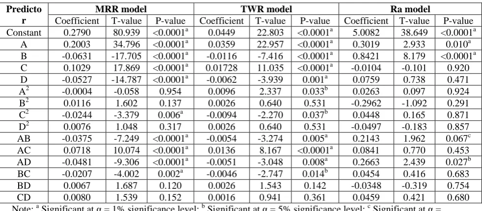
Based on the model described by Eq. (8) and by applying the LSM, all the regression coefficients pertaining to the three responses have been obtained and are shown in Table 5 along with their corresponding Student T- and P-values as a pooled ANOVA format. As is clear from this Table, all the main effects of four input parameters (A: discharge current, B: pulse on-time, C: duty cycle, and D: gap voltage) are found to be highly significant at least at a α = 0.01 significance level or 99% confidence interval, having almost zero P-values in affecting both the MRR and TWR. However, for the third response, Ra, just the first two factors, discharge current (A) and pulse-on time (B) are regarded as the highly significant main factors. In the terminology of statistical modeling, the lower the P-value, the more influential is the effect [29-31]. On the other hand, the pure quadratic effect of duty cycle (C2), the two-way interactions of discharge current with pulse-on time (A×B), with duty cycle (A×C), and with gap voltage (A×D), as well as the interaction amongst the pulse on-time with duty cycle (B×C) were also found to be extremely important terms influencing MRR. For the TWR measure, the dual interactive effects amid current with pulse-on time (A×B), with duty cycle (A×C), and with gap voltage (A×D) plus pulse on-time and duty cycle (B×C) along with the second order effects of discharge current (A2) and duty cycle (C2) were made known to have influencing outcomes. Finally, for the Ra quality measure, the only considerable interactive terms are discharge current with pulse-on time (A×B) and with gap voltage (A×D). As a whole, the inclusion of any term with a P-value less than 0.07 designated as an upper bound for statistical significance; i.e., being significant within 93% of confidence interval, has been guaranteed in this research so as to increase each model’s accuracy and adequacy as high as possible. All the other terms not meeting such a criterion are supposed to be insignificant. Generally, the term “interaction” means that the effect of a factor over a known response depends on the level of another factor. Identifying significant interaction terms in RSM model building procedure and their inclusions in the structure of a second order model are of vital importance as they can reveal very crucial phenomena of the combinatorial joint effects of different process parameters on every process characteristics and behavior [29-31].
Removing insignificant terms is a common practice amongst empirical model builders which, in most cases, can result in improved model fitting capabilities aside from yielding simpler model form. Thereupon, the insignificant terms have been excluded from the models’ structures through backward elimination method [29-31] and the ANOVA has been repeated for every obtained reduced quadratic model containing only those significant terms contributing to model building.
Table 5. Regression coefficients and T-test results for the individual MRR, TWR, and Ra model parameters
Predicto r
MRR model TWR model Ra model
Coefficient T-value P-value Coefficient T-value P-value Coefficient T-value P-value Constant 0.2790 80.939 <0.0001a 0.0449 22.803 <0.0001a 5.0082 38.649 <0.0001a
A 0.2003 34.796 <0.0001a 0.0359 22.957 <0.0001a 0.3019 2.933 0.010a B -0.0631 -17.705 <0.0001a -0.0116 -7.416 <0.0001a 0.8421 8.179 <0.0001a C 0.1029 17.869 <0.0001a 0.01728 11.035 <0.0001a -0.0104 -0.101 0.920 D -0.0527 -14.787 <0.0001a -0.0062 -3.939 0.001a 0.0759 0.738 0.471
A2 -0.0004 -0.058 0.954 0.0096 2.337 0.033b 0.0263 0.097 0.924
B2 0.0116 1.602 0.137 0.0026 0.640 0.531 -0.2962 -1.092 0.291
C2 -0.0244 -3.379 0.006a -0.0094 -2.270 0.037b 0.0448 0.165 0.871
D2 0.0076 1.048 0.317 0.0026 0.640 0.531 -0.0497 -0.183 0.857
AB -0.0375 -7.249 <0.0001a -0.0054 -3.274 0.005a 0.2143 1.962 0.067c AC 0.0718 10.074 <0.0001a 0.0136 8.167 <0.0001a 0.0841 0.770 0.453 AD -0.0481 -9.306 <0.0001a -0.0051 -3.048 0.008a 0.2663 2.439 0.027b
BC -0.0207 -4.002 0.002a -0.0046 -2.747 0.014b 0.0454 0.416 0.683
BD 0.0067 1.687 0.120 0.0026 1.543 0.142 -0.0348 -0.319 0.754
CD 0.0080 1.539 0.152 0.0016 0.941 0.361 0.0459 0.421 0.680
Note: a Significant at α = 1% significance level; b Significant at α = 5% significance level; c Significant at α = 7% significance level
Table 6 illustrates the ANOVA results for the three response functions. As are desired, all the quadratic regression models are significant while their lacks of fits were turned out to be insignificant relative to pure error. Hence, the model adequacy checking is completely assured for each output measure. Other statistical diagnostic indices mainly used to evaluate the modeling goodness of fit are the ordinary R-squared (R2), adjusted R-squared (R2Adj), and predicted R-squared (R2Pred) [30], shown inside Table 6 for every response
model. The values are 99.74%, 99.59%, and 98.51% for MRR; 97.58%, 96.38%, and 91.13% for TWR; and 80.93%, 77.12%, and 74.1% for Ra, respectively. As a general rule, the more the R2s approach unity, the better the model fits the experimental data [29-31]. The usual statistic R2, also called the coefficient of multiple determination, indicates how many percent of the total variations can be explained by the model while the R2Adj,
can be explained by the model after considering the significant terms (reduced model). The amount of R2 increases as each additional variable or regressor, whether significant or insignificant, is added to the model. On the contrary, the adjusted R2 does not automatically increase when new predictor variables are added to the model. In fact, the value of adjusted R2 will often decrease when unnecessary terms are included. Accordingly, when R2 and R2Adj differ dramatically, there is a good chance that nonsignificant terms have been incorporated
in the model [29-31]. Therefore, it is a suitable criterion in evaluating a model’s goodness of fit when only significant terms are involved compared to the case when all the terms are caught up. The statistic PRESS (prediction error sum of squares) is a measure of how well the model will predict new data. A model with a small value of PRESS is desired as it indicates that the model is likely to be a good predictor [30]. In connection with this, the predicted R2 (R2Pred) is defined which is an indication of the predictive capability of regression
model in response to new observations.
The R2s coefficients and PRESS statistic are calculated as:
1 (10)
1 // 1 1 1 (11)
1 (12)
∑ ∑ (13)
where, SSR is the regression sum of squares, SST is the total sum of squares, SSRes is the residual sum of squares, MSRes is the residual mean square, MST is the total mean square, and is the predicted value of the ith
observed response based on a model fit to the remaining (n-1) sample points. More details can be found in [29-31]. A broad overview of these indices confirms suitability and completeness of all the obtained models as neither inconsistency nor poor adequacy can be observed.
Table 6. ANOVA table for the trimmed MRR, TWR, and Ra second order models
Source D F
Seq SS Adj MS F value P
value
Remarks (a) For MRR
Regression 9 1.05761 0.11751 676.09 0.000 Significant
Linear 4 0.98063 0.22721 1307.20 0.000
Square 1 0.00825 0.00066 3.79 0.069
Interaction 4 0.06874 0.01718 98.86 0.000 Residual error 16 0.00278 0.00017 - -
Lack-of-fit 10 0.00250 0.00021 1.68 0.271 Insignificant
Pure error 6 0.00073 0.00012 - - Correlation Total 25 1.06039 - - -
R2 = 99.74% R2Adj = 99.59% R2Pred = 98.51% PRESS = 0.01577
(b) For TWR
Regression 10 0.03641 0.00364 80.76 0.000 Significant
Linear 4 0.03174 0.00794 176.02 0.000
Square 2 0.00051 0.00025 5.64 0.011
Interaction 4 0.00415 0.00104 23.07 0.000 Residual error 20 0.00090 0.00005 - -
Lack-of-fit 14 0.00079 0.00006 3.09 0.086 Insignificant
Pure error 6 0.00011 0.00002 - -
Correlation Total 30 0.03731 - - - -
R2 = 97.58% R2Adj = 96.38% R2Pred = 91.13% PRESS = 0.00331
(c) For Ra
Regression 5 16.379 3.2758 21.22 0.000 Significant
Linear 3 14.510 4.8365 31.33 0.000
Interaction 2 1.870 0.9348 6.06 0.007 Residual error 25 3.859 0.1544 - -
Lack-of-fit 9 1.942 0.2158 1.80 0.146 Insignificant
Pure error 16 1.917 0.1198 - -
Correlation Total 30 20.239 - - -
Table 7 also details all the numerical values of finalized individual regression coefficients for every response. Based on these, the mathematical equations are conformed for each performance characteristics to suitable coefficients and can be expressed in terms of coded factors as:
0.282 0.194 0.063 0.110 0.051 0.014 0.041 0.076 0.042
0.017 (14)
0.045 0.036 0.012 0.017 0.006 0.012 0.007 0.005 0.014
0.005 0.005 (15)
4.849 0.302 0.842 0.076 0.214 0.266 (16)
The above developed models can be used as reliable tools navigating the design space within the process parameters domain to get an in-depth understanding of process characteristics and can also be utilized in the optimization stage to find optimum EDMing conditions on WC-6%Co.
Table 7. Finalized regression coefficients of the response models
Coefficient MRR (g/h) TWR (g/h) Ra (µm) β0 (intercept)
0.2819 0.0454 4.8486
βA 0.1937 0.0359 0.3019
βB -0.0631 -0.0116 0.8421
βC 0.1096 0.0173 Insignifica nt
βD -0.0510 -0.0062 0.0759*
Insignifica nt
0.0119 Insignifica nt
-0.0139 -0.0071 Insignifica nt
-0.0413 -0.0054 0.2143 0.0755 0.0136 Insignifica
nt
-0.0423 -0.0051 0.2663 -0.0168 -0.0046 Insignifica
nt *
Note: The effect of gap voltage (D) on surface roughness is insignificant (see Table 5) and its coefficient has just been kept to comply with the hierarchy principle.
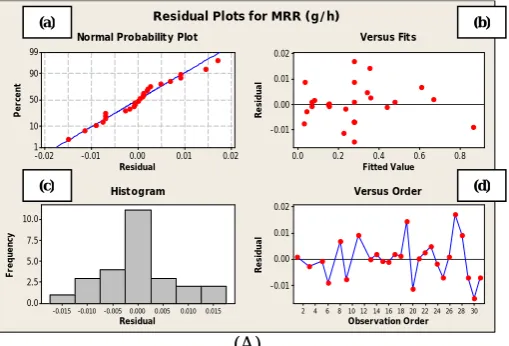
A complete residual analysis has also been done for every developed response and the graphs are shown in Figure 5 (A-C). Normal probability plot of residuals reveals that experimental data are spread approximately along a straight line, confirming a good correlation between experimental and predicted values for the response (Figure 5, A(a), B(a), and C(a)). In graph of residuals versus fitted values (Figure 5, A(b), B(b), and C(b)), only small variations can be seen. The histogram of residuals (Figure 5, A(c), B(c), and C(c)) also shows a Gaussian distribution which is desirable, and finally, in residuals against the order of experimentations in Figure 5, A(d), B(d), and C(d) both negative and positive residuals are apparent indicating no special trend which is worthy from statistical point of view. As a whole, all the yielded models do not show any inadequacy.
0.02 0.01 0.00 -0.01 -0.02 99 90 50 10 1 Residual Pe rc en t 0.8 0.6 0.4 0.2 0.0 0.02 0.01 0.00 -0.01 Fitted Value Re si d ua l 0.015 0.010 0.005 0.000 -0.005 -0.010 -0.015 10.0 7.5 5.0 2.5 0.0 Residual Fr eq ue nc y 30 28 26 24 22 20 18 16 14 12 10 8 6 4 2 0.02 0.01 0.00 -0.01 Observation Order Re si dua l
Normal Probability Plot Versus Fits
Histogram Versus Order
Residual Plots for MRR (g/h)
(A)
(a) (b)
0.01 0.00 -0.01 -0.02 99 90 50 10 1 Residual Pe rc en t 0.16 0.12 0.08 0.04 0.00 0.01 0.00 -0.01 -0.02 Fitted Value Re si d ua l 0.010 0.005 0.000 -0.005 -0.010 -0.015 10.0 7.5 5.0 2.5 0.0 Residual F re que nc y 30 28 26 24 22 20 18 16 14 12 10 8 6 4 2 0.01 0.00 -0.01 -0.02 Observation Order Re si du a l
Normal Probability Plot Versus Fits
Histogram Versus Order
Residual Plots for TWR (g/h)
(B) 1.0 0.5 0.0 -0.5 -1.0 99 90 50 10 1 Residual Pe rc en t 6 5 4 0.8 0.4 0.0 -0.4 -0.8 Fitted Value Re si d ua l 0.8 0.6 0.4 0.2 0.0 -0.2 -0.4 -0.6 8 6 4 2 0 Residual Fr eq ue n cy 30 28 26 24 22 20 18 16 14 12 10 8 6 4 2 0.8 0.4 0.0 -0.4 -0.8 Observation Order Re si d ua l
Normal Probability Plot Versus Fits
Histogram Versus Order
Residual Plots for Ra (micron)
(C)
Figure 5. Plot of residuals: (A) MRR, (B) TWR, (C) Ra
((a) normal probability plot of residuals, (b) residuals versus the fitted values, (c) histogram of the residuals, and (d) residuals against the order of data)
4. Results and discussion
To genuinely describe the quality of variation trends of each process response with respect to inputs, it is of great importance to be aware that spark energy is the dominant factor most responsible for the mechanism of material removal in EDM. The amount of discharge energy (q) delivered per single discharge assuming a normal pulse (i.e. spark) can be expressed as [33]:
. . . . (17)
where Td, Ton, Vdis, and Idis represent the ignition delay time, pulse on-time, discharge voltage and current,
respectively. The magnitude of ignition delay time in normal pulses is so small compared to pulse on-time [34], so its effects has been neglected for the sake of simplicity. In real EDM conditions, for a sequence of electrical discharges occurring between the two electrodes within the total machining time (T), the total discharge duration (TD) is given by:
(18) where DC is the duty cycle (Equation (1)). On the other hand, the whole number of discharge pulses (N) during total machining time can be calculated as:
(19)
Therefore, the total discharge energy (Q) during overall machining time is given by:
. . . (20)
This is the total electrical discharge energy delivered into the gap zone which is then shared between the tool and workpiece electrodes as well as dielectric liquid. All the following discussions are based on this simple relation describing the whole generated electro-thermal energy during sparking, expressed in terms of the selected input EDM parameters.
(a) (b)
(c) (d)
(a) (b)
4.1. Parametric analysis of MRR
Figure 6 shows the main effect plot of each variable on MRR. As is clear, the MRR increases steadily with the increase of discharge current. Higher levels of discharge currents result in more strong electrical discharges (see Eq. 20) capable of removing a chunk of material from the workpiece, hence boosting the rate of erosion [35]. The MRR tends to decrease with the increase of pulse time. Despite the usual belief that longer pulse on-times provide much more on-times for electrical discharging compared to shorter ones, however, in reality, longer pulse durations cause the plasma channel to expand excessively thus lowering the plasma flushing efficiency and electrical discharge density within the gap space with more molten material resolidifying instead of being effectively removed [36, 37]. On the contrary, the main effect of duty cycle displays a reverse tendency. At a constant level of pulse on-time (B=0, or the middle value), increasing duty cycle means lowering the pulse off-time, thereby decreasing the idle time between successive sparks which produces higher discharging frequency leading to higher removal rate. Finally, it can be inferred from the main effect plot of gap voltage that higher MRR is attainable at lower levels of gap voltage. Higher gap voltage provides wider gap distance which in turn results in diminished electrical discharge density and larger gap electrical resistivity hindering proper transmissivity of sparks [37]. So, the MRR decreases with the increase of gap voltage alone. It should noted that these results have been acquired considering the effect of each factor independently (keeping the other parameters unchanged), nevertheless, more practically beneficial outcomes are to be revealed when their mutual joint effects are investigated simultaneously as can be obtained studying 3D surface and 2D contour plots of response measures with respect to each pair of significant input variables.
The combination effect of discharge current (A) and pulse on-time (B) at a constant level (middle value) of duty cycle (C) and gap voltage (D) has been shown in Figure 7 (a) and (b) in 3D surface and 2D contour format. It can be concluded that higher MRRs are achievable at the lower right region of contour plot area where the discharge current is at its maximum value while pulse on-time at minimum adjustable levels within the domain of process parameters considered in this research.
1 0 -1 0.60 0.45 0.30 0.15 0.00
1 0 -1
1 0 -1 0.60 0.45 0.30 0.15 0.00
1 0 -1 A (I)
Me
a
n
B (Ton)
C (DC) D (V)
Main Effects Plot for MRR (g/h)
Data Means
Figure 6. Main effect plots for MRR
(a) (b)
Figure 7. Response surface plot (a) and contour plot (b) of MRR versus current (A) and pulse on-time (B)
This phenomenon can be best attributed to the increased energy density of discharge channel (J) relative to I and
Ton given by [38]:
1
0.0 0
0.2 0.4
-1 0.6
0 -1
1
MRR (g/h)
B (Ton)
A (I)
C (DC) 0 D (V) 0 Hold Values
Surface Plot of MRR (g/h) vs B (Ton); A (I)
0.52
0.47 0.42
0.37 0.32
0.27 0.22
0.17 0.12
A (I)
B (
T
o
n
)
1.0 0.5 0.0 -0.5 -1.0 1.0
0.5
0.0
-0.5
-1.0
(21)
where, a, b, and k are constant coefficients. Although the discharge energy itself is small with a short pulse on-time (Eq. 17), due to a very small discharge channel diameter a higher discharge density is expected. Hence, the higher the discharge current and the lower the pulse on-time the larger is the electrical discharge density. Higher discharge density causes most of the material in the discharge area to be removed in the form of evaporation with thinner recast layer left on the work surface increasing the plasma flushing efficiency [39] and hence the MRR.
Figure 8 illustrates the effect of current (A) and duty cycle (C) on MRR. It is understood that while keeping pulse on-time and gap voltage at a certain level, middle level in our case, higher amounts of MRR are achievable mostly in the vicinity specified by both elevated current and duty cycle. At a steady pulse on-time, increased duty cycle implies lower pulse off-time, when combined with elevated discharge currents; higher rates of electrical discharge energy are assured making the MRR as large as possible. Figure 9 depicts the effect of current (A) and gap voltage (D) whereas Figure 10 shows the mutual effect of pulse on-time (B) and duty cycle (C) on MRR while keeping the other variables at their center levels unvarying. It becomes clear that higher values of current along with lower gap voltage will definitely provide a suitable medium for higher amounts of material melting and evaporation during sparking thanks to enhanced electrical discharge density in a narrower gap region. Lowering the pulse on-time and increasing duty cycle convey greater discharge frequency in which more material can be removed from the work piece in a unit time [28]. This event is clearly visible in Figure 10.
(a) (b)
Figure 8. Response surface plot (a) and contour plot (b) of MRR versus current (A) and duty cycle (C)
(a) (b)
Figure 9. Response surface plot (a) and contour plot (b) of MRR versus current (A) and gap voltage (D)
0.60
0.54 0.48
0.42 0.36
0.30 0.24
0.18 0.12
0.06
A (I)
C (
DC
)
1.0 0.5 0.0 -0.5 -1.0 1.0
0.5
0.0
-0.5
-1.0
B (T on) 0 D (V) 0 Hold Values Contour Plot of MRR (g/h) vs C (DC); A (I)
1
0.0 0
0.2 0.4
-1 0.6
0 -1
1
MRR (g/h)
C (DC)
A (I)
B (Ton) 0 D (V) 0 Hold Values Surface Plot of MRR (g/h) vs C (DC); A (I)
0.530 0.489
0.448 0.407
0.366 0.325
0.284 0.243
0.202 0.161
0.120
A (I)
D (V)
1.0 0.5 0.0 -0.5 -1.0 1.0
0.5
0.0
-0.5
-1.0
B (T on) 0 C (DC) 0 Hold Values Contour Plot of MRR (g/h) vs D (V); A (I)
1
0 0.2
0.4
-1 0.6
0 -1
1
MRR (g/h)
D (V)
A (I)
B (T on) 0 C (DC) 0 Hold Values
(a) (b)
Figure 10. Response surface plot (a) and contour plot (b) of MRR versus pulse on-time (B) and duty cycle (C)
4.2. Parametric analysis of TWR
Figure 11 shows the four main effect plots of TWR model each of which has been drawn keeping the other factors constant at the middle level. A similar trend is observed compared to the main effect plots of MRR. The TWR tends to increase by increasing discharge current and can reach up to about 0.09 g/h alone. This is the highest amount of TWR in these plots which in turn confirms that the discharge current is paramount amongst other parameters in affecting the TWR. It is clear from the main effect plot of pulse on-time that setting longer pulse on-times can favor it as shorter pulse durations will deteriorate tool wear. To better justify this fact, Figure 12 illustrates a schematic view of a single electrical discharge happening between the two electrodes and the formed plasma channel. While keeping constant polarity, during every discharge, accelerated electrons bombard the surface of anode (positive pole: tool) whereas ions aiming to move toward the cathode (negative pole: work piece) collide the work surface. With small values of pulse duration, a higher number of negatively charged particles, being thousands of times lighter than ions, get the chance of being energized; stroke the positive (anode) tool electrode thereby increasing the rate of electrode material erosion [40]. On the same basis, the rising tendency of TWR with regard to duty cycle can be rationalized. A higher level of duty cycle is equivalent to lower pulse off-time and hence higher pulse frequency which implies greater TWR due to privileged rate of electron collisions with the anode tool surface [28]. On the other hand, selecting lower gap voltage results in larger tool wear rate. The same reason as that mentioned for the MRR can surely be applied here. While keeping other variables unchanged, a narrower gap distance caused by selecting a smaller gap voltage, will give rise to increased electrical discharge density leading to higher rate of tool wear.
The TWR response surface plot and its corresponding contour plot with regard to current (A) and pulse on-time (B) has been depicted in Figure 13. As always smaller TWRs are demanded, they can be reached at lower discharge currents followed by longer pulse on-times (the upper left part of the contour plot). Prolonged pulse duration will give more chance for much heavier positive ions to reach to the target cathode work piece thus occupying most of the plasma channel path not letting excited electrons attacking the anode tool [41]. Besides, at long pulse duration, the released carbon resulting from the decomposition of hydrocarbon-based dielectric liquid, due to high plasma temperature during sparking, attaches to the tool’s surface forming a protective layer against wear, and hence decreasing the TWR perceptibly [42].
1 0 -1 0.08
0.06 0.04 0.02
1 0 -1
1 0 -1 0.08
0.06 0.04 0.02
1 0 -1 A (I)
Me
a
n
B (Ton)
C (DC) D (V)
Main Effects Plot for TWR (g/h)
Data Means
Figure 11. Main effect plots for TWR
0.44 0.41
0.38
0.35
0.32
0.29
0.26
0.23
0.20
0.17
0.14
B (Ton)
C (D
C)
1.0 0.5 0.0 -0.5 -1.0 1.0
0.5
0.0
-0.5
-1.0
A (I) 0 D (V) 0 Hold Values Contour Plot of MRR (g/h) vs C (DC); B (Ton)
1
0.1 0
0.2 0.3 0.4
-1
0 -1
1
MRR (g/h)
C (DC)
B (Ton)
Figure 12. Schematic drawing of a single electrical discharge
(a) (b)
Figure 13. Response surface plot (a) and contour plot (b) of TWR versus current (A) and pulse on-time (B)
Figure 14 shows the effect of discharge current (A) and duty cycle (C) on TWR. It is noticeably revealed that smaller TWRs (less than 0.03 g/h) can be obtained by specially a combination of a range of low to medium discharge currents with almost any arbitrarily chosen value of the duty cycle (the end left side of contour plot), and that much smaller TWRs are accomplished moving toward the minimum current (A = -1). This fact, however, cannot be elicited solely by checking the main effect plots of duty cycle and current as both present the same influence on TWR, increasing each of which makes the TWR to increase progressively. This is undoubtedly due to the strong interactive nature of these two parameters suitably found by the ANOVA on TWR response (see Table 5). Moreover, the tool electrode suffers more from wear where the current and duty cycle are both chosen at their high levels, a zone located at the upper right part of the contour plot. Increasing duty cycle at a steady level of pulse on-time (the case where Figure 14 has been drawn) means lowering pulse off-time and so increasing the frequency of electrical discharges assuring higher rates of electron attacks on anode tool electrode in a unit time. Similar results have also been reported by Iuras [40].
Figure 15 (a) and (b) displays the effects of current (A) and gap voltage (D) as surface and contour plot. As can be inferred from the contour plot, low TWRs may be accessible with small currents accompanied by every adjustable level of gap voltage within the current study. In other words, the coincident effects of these two factors on TWR counteract the effect of gap voltage alone shown in Figure 11, as now a wide range of it can be selected to yield small TWR provided that the current is kept low enough. This can be attributed to the stronger and more influential effect of current (A) over the TWR as having a much smaller p-value compared to the gap voltage (D) (refer to Table 5), covering the effect of gap voltage when considered in a combinatory way. Figure 16 shows the concurrent effect of pulse on-time (B) and duty cycle (C). It is obviously visible that smaller TWRs can be obtained choosing a higher level of pulse on-time with lower duty cycle. This combination confirms decreased sparking frequency meaning lower amount of electron attack to the positive-polarity tool electrode in a unit time causing less tool wear rate [35].
0.095
0.087 0.079
0.071 0.063
0.055 0.047
0.039 0.031
0.023
A (I)
B (
T
o
n
)
1.0 0.5 0.0 -0.5 -1.0 1.0
0.5
0.0
-0.5
-1.0
C (DC) 0 D (V) 0 Hold Values Contour Plot of TWR (g/h) vs B (Ton); A (I)
1 0.03
0 0.06
0.09
-1 0.12
0 -1
1
TWR (g/h)
B (Ton)
A (I)
(a) (b)
Figure 14. Response surface plot (a) and contour plot (b) of TWR versus current (A) and duty cycle (C)
(a) (b)
Figure 15. Response surface plot (a) and contour plot (b) of TWR versus current (A) and gap voltage (D)
(a) (b)
Figure 16. Response surface plot (a) and contour plot (b) of TWR versus pulse on-time (B) and duty cycle (C)
4.3. Parametric analysis of Ra
Figure 17 depicts the main effect plots of the four controllable parameters on Ra. It is understandable that the first two variables, current (A) and pulse on-time (B), have more influential impacts on Ra than those of duty cycle (C) and gap voltage (D). More specifically, increasing the pulse on-time alone, while keeping the other factors constant at their middle levels, can increase Ra from 4 µm up to about 5.7 µm which is a higher
0.068 0.063 0.058 0.053 0.048 0.043 0.038 0.033 0.028 0.023 0.018 B (Ton) C (D C) 1.0 0.5 0.0 -0.5 -1.0 1.0 0.5 0.0 -0.5 -1.0
A (I) 0 D (V) 0 Hold Values Contour Plot of TWR (g/h) vs C (DC); B (Ton)
1 0.03 0 0.06 0.09 -1 0 -1 1 TWR (g/h) D (V) A (I)
B (Ton) 0 C (DC) 0 Hold Values Surface Plot of TWR (g/h) vs D (V); A (I)
0.088 0.080 0.072 0.064 0.056 0.048 0.040 0.032 0.024 A (I) D ( V) 1.0 0.5 0.0 -0.5 -1.0 1.0 0.5 0.0 -0.5 -1.0
B (Ton) 0 C (DC) 0 Hold Values Contour Plot of TWR (g/h) vs D (V); A (I)
1 0.02 0 0.04 0.06 -1 0.08 0 -1 1 TWR (g/h) C (DC)
B (Ton)
A (I) 0 D (V) 0 Hold Values Surface Plot of TWR (g/h) vs C (DC); B (Ton)
1 0.00 0 0.04 0.08 -1 0.12 0 -1 1 TWR (g/h) C (DC) A (I)
B (Ton) 0 D (V) 0 Hold Values Surface Plot of TWR (g/h) vs C (DC); A (I)
0.10 0.09 0.08 0.07 0.06 0.05 0.04 0.03 0.02 A (I) C (D C) 1.0 0.5 0.0 -0.5 -1.0 1.0 0.5 0.0 -0.5 -1.0
difference interval than those created by other parameters. As also clear, altering both the duty cycle (C) and gap voltage (D) within their designated intervals considered in this research causes little change on the Ra. This fact was also verified before (see Table 5) as not being significant parameters within 95% of confidence interval, and their main effect diagrams have just been shown here for comparative purposes. In general, the surface quality in EDM depends primarily on the magnitude of electrical discharge energy governed mainly by current intensity and pulse on-time [42, 43]. A prolonged pulse on-time makes discharging action to continue over a longer time duration so that deeper and broader craters are formed over the work surface overwhelming with abundance of resolidified molten material not being ejected effectively which in turn leads to worsened and coarser surface quality [36, 39].
1 0 -1 5.6 5.2 4.8 4.4 4.0
1 0
-1
1 0 -1 5.6 5.2 4.8 4.4 4.0
1 0
-1 A (I)
Me
a
n
B (Ton)
C (DC) D (V)
Main Effects Plot for Ra (micron)
Data Means
Figure 17. Main effect plots for Ra
Figure 18 illustrates the joint effects of pulse current (A) and pulse on-time (B) over the Ra. It is apparent that smoother surfaces can be obtained allocating both small values for pulse on-time and discharge current, a situation identified as low energy state. For example, according to the Figure 18 (b), if it is desired to produce a surface having 4.25 µm as Ra roughness, then it is feasible by choosing any arbitrary value for the discharge current within its investigated domain provided that the pulse on-time is allotted to vary from -1 to about -0.5 in coded state (50 µs to 75 µs). However, still smoother surfaces may be achieved by narrowing down their variation ranges toward minimum levels.
Figure 19 (a) and (b) portray the surface and contour plot of Ra with respect to discharge current (A) and gap voltage (D). From this, it is recommended to apply low currents with high levels of gap voltage (the upper left part of Figure 19(b)) at a constant level of pulse on-time to produce more polished work surfaces. Higher gap voltage, while making the gap distance wider facilitating debris removal from the gap space, can help reduce electrical discharge density, altogether with low current intensity collaborate in attaining a superior surface quality [36].
(a) (b)
Figure 18. Response surface plot (a) and contour plot (b) of Ra versus discharge current (A) and pulse on-time (B)
6.05 5.85
5.65 5.45
5.25 5.05
4.85 4.65
4.45 4.25
4.05
A (I)
B (
T
o
n
)
1.0 0.5 0.0 -0.5 -1.0 1.0
0.5
0.0
-0.5
-1.0
D (V) 0 Hold Values Contour Plot of Ra (micron) vs B (Ton); A (I)
1 4
0 5
-1 6
0 -1
1
Ra (micron)
B (Ton)
A (I)
(a) (b)
Figure 19. Response surface plot (a) and contour plot (b) of Ra versus discharge current (A) and gap voltage (D)
5. Multi-objective optimization of EDM parameters based on desirability function
Metal removal rate is an indicator for productivity while tool wear rate and surface finish account for process economics, precision, and work quality. In particular, tool wear is of paramount concern especially when close tolerances in intricate geometries are needed. The EDM, as a complex and stochastic process, exhibits much difficulty in determining optimal machining parameters for best machining performance. The performance indicators, viz. MRR, TWR, and Ra are conflicting in nature as it is always desirable to have higher MRR with a lower value of surface roughness and tool wear rate at the same time. Due to the presence of a large number of process variables and mutual interactions, the selection of optimum machining parameter combinations to obtain higher MRR and smaller SR and TWR is a challenging task [44]. Here, an attempt is made to develop a strategy based on the concept of desirability function for predicting the optimum machining parameter settings generating maximum MRR with minimum SR and TWR all at once.
5.1. Optimization formulation
The mathematical formulation of the present optimization problem can be stated as follow:
: : :
: 2 8
50 150 (22) 40 80
40 80
where, x1, x2, x3, and x4 represent the process input parameters I, Ton, DC, and V, respectively. It is a
four-variable-three-objective optimization statement, each of which has been defined by respective second order regression equations, Equations (14-16).
5.2. Optimization through desirability function
Popularized by Derringer and Suich [45], the desirability function approach (DFA) is a kind of search-based optimization method capable of handling several response functions simultaneously to find optimal input settings globally. The overall approach is to first convert each response yi into an individual desirability function di that varies over the range:
0 1 (23)
If the response yi is at its goal or target, then di = 1 (the most desirable case), and if the response is outside an
acceptable region, di = 0 (the least desirable case). There is also a positive number, weight factor (r), associated
with the desirability function of each response defining its shape. If the weight is chosen to be less than 1, then the sensitivity of the desirability function is low with respect to the optimal or target value sought for. In other words, if the search algorithm finds a point which is somehow far from the desired optimum or target value, then the decrease in desirability function value will be small in comparison with its maximum amount (unity). Choosing a weight factor higher than one, has the reverse effect, and setting it to one, provides a balanced or medium sensitivity with the shape of desirability being linear [29, 46]. The individual desirability functions are defined according to the goal of optimization and are shown in Figure 20 (a) and (b) for the two cases, maximization and minimization, respectively.
5.4 5.3
5.2 5.1
5.0 4.9
4.8 4.7
4.6 4.5
A (I)
D (
V
)
1.0 0.5 0.0 -0.5 -1.0 1.0
0.5
0.0
-0.5
-1.0
B (T on) 0 Hold Values Contour Plot of Ra (micron) vs D (V); A (I)
1 4.5
0 5.0
-1 5.5
0 -1
1
Ra (micron)
D (V)
A (I)
B (Ton) 0 Hold Values
If the objective or target Ti for the response yi is a maximum value, then: 0
1
(24)
and if the target for the response is a minimum value, then:
1
0
(25)
where, Li and Ui represent the lower and upper limit values of the response yi, respectively.
(a) (b)
Figure 20. Individual desirability functions for simultaneous optimization: (a) objective is to maximize y, (b) objective is to minimize y
The individual desirabilities are then combined to form the overall (composite or aggregated) desirability (D), another parameter varying between 0 and 1, as the weighted geometric mean of all the previously defined desirability functions, given by:
… ∏ ∑ (26)
where wi is the relative importance, a comparative scale for weighting each of the resulting di, assigned to the ith
response and n is the number of responses (n = 3, in our case). The optimal settings are determined so as to maximize the overall desirability (D) by usually applying a reduced gradient algorithm with multiple starting points [47].
5.3. Parametric optimization of the EDM process on WC-6%Co
Based on the developed quadratic mathematical responses (Eq. 14-16), d1, d2, and d3 are selected as the
independent desirability functions for the MRR, TWR, and Ra, respectively. Moreover, the targets are placed on the MRR to become maximized while TWR and Ra to be minimized. Unit weight factor (r = 1) and importance (wi = 1) were also assigned for each response. The Response Optimizer option within the DOE module of
Conducting confirmation experiment is the crucial, final, and indispensable part of every optimization attempt. Verification experiment was performed at the obtained optimal input parametric setting to compare the actual MRR, TWR, and Ra with those as optimal responses got through desirability approach. Table 10 summarizes the optimization results along with experimentally obtained responses and their percentage relative verification errors. It should be noted that the errors have been calculated as:
% 100 (27)
As is clear, the amounts of errors are all found to be satisfactory in point of engineering applications, 10.64% as the worst case in predicting TWR, assuring the feasibility, predictability, and effectiveness of the adopted approach.
Table 8. Constraints and criteria of input parameters and responses
Parameter/Resp onse Goal Lower limit Upper limit Discharge current In
range
2 8
Pulse on-time In range
50 150
Duty cycle In range
40 80
Gap voltage In range 40 80 Material removal rate Maximi ze 0.02 0.86
Tool wear rate Minimi ze 0.007 0.15 Surface roughness Minimi ze 3.395 6.589
Table 9. Iterative determination of optimum conditions (inputs in coded form)
Soluti on Curren t (A) Pulse on-time (B) Duty cycle (C) Gap voltage (D) MRR (g/h) TWR (g/h) Ra (µm)
d1 d2 d3 Composi
te desirabil
ity (D)
1 0.23232 3
-0.989478 -1 -1 0.301
87
0.042 41
3.898 37
1 1 1 1
2 0.43434 3
-0.959596 -1 -0.959596 0.337 82 0.050 02 3.898 41 1 0.9996 04 1 0.999868 3 -0.39705 9
-1 1 1 0.3 0.047
63
3.941 84
1 1 0.96195
9
0.987155
4 -0.50192
7
-0.942816 1 -1 0.327
98
0.05 4.062 18
1 1 0.85256
2
0.948219
5 0 -1 0 0.881845 0.3 0.051
58 4.073 41 1 0.9684 6 0.84235 6 0.934385 6 0.64352 8 -1 0.93043 1 0.419331 0.288 49 0.05 4.166 54 0.8849 4 0.9999 84 0.75769 0.875251
7 0.43614 -1
-0.59935 3 0.970432 0.279 56 0.05 4.231 07 0.7955 89 0.9999 98 0.69902 6 0.822357 8 -0.15712 9
-0.476585 1 1 0.325
88
0.05 4.449 91
1 1 0.50007
8
0.793742
9 0.99758 7
-1 -1 1 0.270
54 0.056 4 4.435 47 0.7054 21 0.8719 67 0.51320 7 0.680895 10 0.34427 5 0.15463 -0.94630 9 -1 0.282 79 0.041 36 4.643 25 0.8278 84 1 0.32432 2 0.645132
Cur
High Low 1.0000D Optimal
d = 1.0000 Maximum MRR (g/h
y = 0.3019
d = 1.0000 Minimum TWR (g/h
y = 0.0424
d = 1.0000 MinimumRa (micr y = 3.8984
1.0000 DesirabilityComposite
-1.0 1.0 -1.0
1.0 -1.0 1.0 -1.0
1.0 B (Ton) C (DC) D (V)
A (I)
[0.2323] [-0.9895] [-1.0] [-1.0]
Figure 21. Final optimization results
Table 10. Multi-response optimal points and experimental validation
Optimum input setting MRR (g/hr) TWR (g/hr) Ra (µm) Relative error (%) I
(A) Ton
(µs)
DC (%)
V (V)
Predic ted
Experim ental
Predic ted
Experim ental
Predic ted
Experim ental
MR R
TW R
Ra 5.7
0
50.53 40 40 0.302 0.331 0.042 0.047 3.898 4.141 8.76 10.6
4 5.8
7
5.4. The interpretation of optimal settings
Making a thorough analysis of the optimum input values can provide a fair basis to justify their estimated amounts in point of physical aspects involved in the EDM process. In the course of optimization through the desirability function approach, a measure of how well the solution has satisfied the combined goals for all responses must be assured. That is D = 1 and the optimum setting providing this could have been able to make a tradeoff between different objective functions. The amount of optimal discharge current has been found to be near to its middle value, providing fair electro-thermal energy so that neither a very low MRR nor an extremely high one is obtained. Along with almost the shortest possible pulse on-time (50.53 µs), the existence of adequate electrical discharge density is assured to help maintaining enough impulsive force expelling much of molten material from crater [48]. Moreover, as was discussed in subsection 4.3, shorter pulse on-times are in favor of smoother surfaces, as the resulted craters’ dimensions (depth and diameter) are smaller compared with those created with long pulse durations. Hence, better surface quality is guaranteed. Finally, the optimal values of duty cycle and gap voltage are equivalent to their lowest possible levels considered in the experimental plan as increasing each of which may cause the process performance to deviate from its optimum condition by sacrificing any of the three responses. This effect can be seen in Table 9. Specially, the lowest gap voltage (40 V) provides the narrower gap distance increasing electrical discharge density inside the gap zone helping to improve the MRR.
6. Conclusions
Conventional machining of the hard metal WC/6%Co composite is extremely laborious, burdensome, and time consuming due to its elevated hardness and brittleness over a wide range of temperatures and working conditions. The effective and economic utilization of EDM process on such a material with optimum selection of input parameters needs a thorough understanding of its machinability behavior which in turn can substantially alleviate the difficulties encountered. In short, based on the in-depth and comprehensive analysis and optimization of WC-6%Co ED-machinability indices, the following principal conclusions can be drawn:
1- All the main effects of input parameters, i.e., discharge current, pulse on-time, duty cycle, and gap voltage were found to be highly significant in affecting both the MRR and TWR. However, for the third response, the Ra, just the main effects of the first two factors (current and pulse on-time) were revealed to be statistically important.