https://doi.org/10.5194/amt-12-51-2019
© Author(s) 2019. This work is distributed under the Creative Commons Attribution 4.0 License.
CALIPSO lidar calibration at 1064 nm: version 4 algorithm
Mark Vaughan1, Anne Garnier1,2, Damien Josset3, Melody Avery1, Kam-Pui Lee1,2, Zhaoyan Liu1, William Hunt1,2,†, Jacques Pelon4, Yongxiang Hu1, Sharon Burton1, Johnathan Hair1, Jason L. Tackett1,2, Brian Getzewich1,2,
Jayanta Kar1,2, and Sharon Rodier1,2
1NASA Langley Research Center, Mail Stop 475, Hampton, VA 23681-2199, USA
2Science Systems and Applications Inc. (SSAI), 1 Enterprise Parkway, Suite 200, Hampton, VA 23666, USA 3US Naval Research Laboratory, NASA Stennis Space Center, MS 39529, USA
4Laboratoire Atmosphères, Milieux, Observations Spatiales, UPMC-UVSQ-CNRS, Paris, France †deceased
Correspondence:Mark Vaughan ([email protected]) Received: 8 September 2018 – Discussion started: 24 September 2018
Revised: 20 November 2018 – Accepted: 29 November 2018 – Published: 3 January 2019
Abstract. Radiometric calibration of space-based elastic backscatter lidars is accomplished by comparing the mea-sured backscatter signals to theoretically expected signals computed for some well-characterized calibration target. For any given system and wavelength, the choice of calibra-tion target is dictated by several consideracalibra-tions, including signal-to-noise ratio (SNR) and target availability. This pa-per describes the newly implemented procedures used to calibrate the 1064 nm measurements acquired by CALIOP (i.e., the Cloud-Aerosol Lidar with Orthogonal Polarization), the two-wavelength (532 and 1064 nm) elastic backscatter lidar currently flying on the Cloud-Aerosol Lidar and In-frared Pathfinder Satellite Observations (CALIPSO) mis-sion. CALIOP’s 532 nm channel is accurately calibrated by normalizing the molecular backscatter from the upper-most aerosol-free altitudes of the CALIOP measurement region to molecular model data obtained from NASA’s Global Modeling and Assimilation Office. However, because CALIOP’s SNR for molecular backscatter measurements is prohibitively lower at 1064 nm than at 532 nm, the direct high-altitude molecular normalization method is not a viable option at 1064 nm. Instead, CALIOP’s 1064 nm channel is calibrated relative to the 532 nm channel using the backscat-ter from a carefully selected subset of cirrus cloud measure-ments. In this paper we deliver a full account of the revised 1064 nm calibration algorithms implemented for the version 4.1 (V4) release of the CALIPSO lidar data products, with particular emphases on the physical basis for the selection of “calibration quality” cirrus clouds and on the new
aver-aging scheme required to characterize intra-orbit calibration variability. The V4 procedures introduce latitudinally vary-ing changes in the 1064 nm calibration coefficients of 25 % or more, relative to previous data releases, and are shown to substantially improve the accuracy of the V4 1064 nm at-tenuated backscatter coefficients. By evaluating calibration coefficients derived using both water clouds and ocean sur-faces as alternate calibration targets, and through compar-isons to independent, collocated measurements made by air-borne high spectral resolution lidar, we conclude that the CALIOP V4 1064 nm calibration coefficients are accurate to within 3 %.
1 Introduction
or-bit inclined at 98◦, acquiring near-continuous measurements between 82◦S and 82◦N on a 16-day repeat cycle (Hunt et al., 2009). CALIOP acquired its first backscatter profiles on 7 June 2006 and has now delivered over 12 years of altitude-resolved measurements of clouds and aerosols in the Earth’s atmosphere.
An essential precondition required to reliably derive the spatial and optical properties of clouds and aerosols from the CALIOP measurements (or from any other Earth-observing elastic backscatter lidar) is the accurate calibration of the measured backscatter data. In particular, accurate calibra-tion of the CALIOP 1064 nm measurements is critically im-portant in subsequent analyses such as reliably discriminat-ing clouds from aerosols (Liu et al., 2018) and in retriev-ing accurate estimates of aerosol optical depths (Young et al., 2013, 2016; Kim et al., 2018). To date, the radiometric calibration of space-based elastic backscatter lidar measure-ments has always been accomplished by calculating time-varying scale factors that provide the best near-instantaneous match between the measured data and the theoretically ex-pected backscatter signals derived for some stable, well-characterized calibration target. The choice of calibration tar-get depends critically on tartar-get availability and the signal-to-noise ratio (SNR) of the target measurements. By far the most common target is the Earth’s atmosphere, which at very high altitudes is essentially free of aerosol contamina-tion, and hence the expected molecular backscatter can be well-characterized using the temperature and pressure pro-files provided by atmospheric model data (e.g., from NASA’s Global Modeling and Assimilation Office – GMAO). The first space-based Earth-observing lidar, the Lidar In-space Technology Experiment (LITE), which flew aboard the space shuttle in September 1994 (Winker et al., 1996), used this high-altitude molecular normalization technique to calibrate the 355 and 532 nm measurements (Osborn, 1998; Osborn et al., 1998). However, because the molecular scattering cross sections at 1064 nm are a factor of∼17 lower than at 532 nm (and∼89 times lower than at 355 nm), the 1064 nm SNR in the high-altitude calibration region precluded the use of the molecular normalization technique for those data. As a con-sequence, the 1064 nm measurements were left uncalibrated in LITE level 1 data distributed by NASA’s Atmospheric Sci-ence Data Center (see https://eosweb.larc.nasa.gov/project/ lite/lite_table, last access: 8 September 2018).
Following the release of the LITE data, Reagan et al. (2002) devised a method to calibrate the 1064 nm chan-nel using the backscatter signals from dense cirrus clouds. The ice crystal sizes within the clouds used by the calibra-tion routines are assumed to be quite large with respect to the laser wavelengths, and hence the in-cloud extinction is concomitantly assumed to be spectrally independent. Reagan et al. (2002) further argue that the cirrus backscatter coeffi-cients are also spectrally independent at 532 and 1064 nm, and thus estimates of the 1064 nm calibration coefficients could be obtained by comparing the uncalibrated 1064 nm
measurements to the calibrated 532 nm measurements of strongly scattering cirrus clouds. The Reagan et al. (2002) technique was subsequently used to calibrate 1064 nm lidar measurements made by the Geoscience Laser Altimeter Sys-tem (GLAS), a two-channel space-based elastic backscatter instrument that launched on 12 January 2003 (Palm et al., 2004; Spinhirne et al., 2005).
The CALIOP 1064 nm calibration scheme also traces its lineage directly back to the pioneering work of Reagan et al. (2002). However, the use of cirrus clouds as a calibration target is not uniformly implemented for all space-based li-dars. Unlike LITE, GLAS, and CALIOP, the Cloud-Aerosol Transport System (CATS) used the molecular normalization technique, together with estimates of aerosol loading pro-vided by CALIOP, to calibrate their 1064 nm measurements over an altitude range of 23 to 27 km (Yorks et al., 2016). This was possible because the CATS instrument design de-livered nighttime SNR in the low-to-middle stratosphere that was substantially higher than in the earlier systems. The CATS transmitters have laser pulse rate frequencies (PRFs) of 4 and 5 kHz, per-pulse energies of 1–2 mJ, and are coupled to receivers that use photon counting detection at 1064 nm. In contrast, CALIOP has a PRF of 20.16 Hz, a nominal per-pulse energy of 100–110 mJ, and detects the backscattered energy at 1064 nm using an avalanche photodiode (APD) (Hunt et al., 2009). While the APD has a relatively high quantum efficiency, it also has a high detector dark count rate, which contributes significant levels of noise in the high-altitude molecular signals. These high noise levels, combined with the greatly reduced sensitivity to molecular scattering, eliminate high-altitude molecular normalization as a viable option for calibrating the CALIOP 1064 nm channel.
Through the course of three major data releases spanning ∼8 years of on-orbit operations, the CALIOP 1064 nm cal-ibration scheme remained relatively unchanged. The theo-retical basis of the original algorithm is given in Hostetler et al. (2005). Vaughan et al. (2010) provide details on some procedural modifications that were incorporated for the ver-sion 3 (V3) data release. In contrast to these V3 updates, the version 4.1 (V4) release is a comprehensive upgrade that fea-tures major changes to all of the primary components of the 1064 nm calibration algorithm. In particular, we
(a) defined a detailed set of sharply focused criteria to iden-tify a much more homogeneous population of clouds used in the calibration procedure;
(b) implemented a wholly new data averaging scheme that reduces uncertainties while simultaneously preserving intra-orbit variations in the calibration coefficients; and (c) augmented the lidar level 1 (L1) data products with sub-stantially more robust estimates of calibration uncer-tainties.
The fundamentals of the CALIOP 532 molecular normal-ization technique are given in Hostetler et al. (2005) (here-after H05) and Powell et al. (2009) (here(here-after, P09). Initial development of CALIOP’s 1064 nm cirrus cloud calibration scheme and the mathematical development of the error prop-agation is given in H05, with postlaunch updates provided in Vaughan et al. (2010) (hereafter V10). The paper is organized as follows. Section 2 reviews the fundamental assumptions and equations that are used in the CALIOP 1064 nm calibra-tion scheme. Seccalibra-tion 3 provides a brief review of the spe-cific techniques used for the V3 data release and highlights the shortcomings that motivated the development of the V4 scheme. Details of the V4 approach, including the physical basis for selecting “calibration quality” cirrus clouds and the constraints involved in developing a multi-orbit data averag-ing scheme, are given in Sect. 4. An in-depth comparison between the V3 and V4 calibration coefficients is conducted in Sect. 5, while Sect. 6 explores a variety of internal consis-tency checks and validation techniques. Concluding remarks are given in Sect. 7.
2 CALIOP 1064 nm calibration fundamentals
The CALIOP 1064 nm calibration scheme uses the calibrated 532 nm attenuated backscatter coefficients measured in cirrus clouds to derive 1064 nm calibration coefficients from the si-multaneously acquired but as yet uncalibrated 1064 nm cir-rus measurements. As described in Sect. 3 of V10, in V3 and earlier the equation used to transfer the 532 nm calibration to the 1064 nm channel is
C1064=FV3C532, (1)
whereC1064andC532are, respectively, the calibration
coeffi-cients at 1064 and 532 nm. The calibration scale factorFV3is
computed using measurements acquired at both wavelengths:
FV3=χcirrus−1
X01064(z)
X5320 (z) !
. (2)
In this expression, X0λ(z) is the background-subtracted, range-corrected, gain- and energy-normalized measured backscatter signal at altitudezand wavelengthλ(i.e., either 532 or 1064 nm), with additional corrections applied to ac-count for molecular and ozone attenuations (V10).
Xλ0(z)is the mean value ofX0λ(z), computed from cloud top to cloud base. In terms of the atmospheric components being mea-sured,
X0λ(z)=Cλ βλ,p(z)+βλ,m(z)Tλ,2p(z) , (3)
where Cλ is the wavelength-dependent calibration coeffi-cient, βλ(z) is the wavelength-dependent backscatter coef-ficient for either particulates (subscript p) or molecules (sub-script m), and T2λ,p(z) is the particulate two-way transmit-tance due to the ice crystals in cirrus clouds. Because these
crystals are quite large relative to the CALIOP wavelengths, the extinction coefficients are assumed to be spectrally inde-pendent, and hence
X01064(z) X0532(z) =
C
1064
C532
β1064,p(z)+β1064,m(z)
β532,p(z)+β532,m(z)
. (4)
The remaining term in Eq. (2),χcirrus, is the mean backscatter
color ratio for cirrus clouds, defined as
χcirrus=
βp,1064(z)
βp,532(z)
, (5)
where the angle brackets once again represent the mean value computed from cloud top to cloud base. Note that when Eq. (4) is applied to appropriately selected cirrus clouds, β1064,p(z)≈β532,p(z)(i.e., the assumption invoked by Rea-gan et al., 2002) andβ532,p(z)β532,m(z), so that the ratio
of the total backscatter coefficients (i.e., molecular and par-ticulate combined) reduces to a very close approximation to the ratio of the particulate backscatter terms alone.
On the right-hand side of Eq. (1), the values of
X0532(z) and
X10640 (z)
used to compute FV3 are obtained directly
from the measured data, andC532 is derived by calibrating
the 532 nm data (Kar et al., 2018; Getzewich et al., 2018). Theχcirrus term inFV3 is an externally prescribed a priori
value, and the only quantity in Eq. (1) that is not directly de-rived from CALIOP’s onboard measurements. For versions 1 and 2 of the CALIPSO data products,χcirruswas assumed to
be 1.00±0.04 (H05). This assumption was revisited and re-vised prior to the release of V3. Based on the analysis of over 400 h of multiwavelength elastic backscatter measurements acquired by the Cloud Physics Lidar (McGill et al., 2002), χcirrusis now assigned a uniform value of 1.01±0.25 for all
CALIOP 1064 nm calibration procedures. Our rationale for this choice is described at length in V10. Recent field ob-servations using the Raman lidar technique at both 532 and 1064 nm provide further evidence for the spectral indepen-dence of cirrus backscatter (Haarig et al., 2016), as do pre-vious elastic backscatter lidar measurements acquired at 550 and 728 nm (Ansmann et al., 1993) and multiwavelength Ra-man measurements acquired at 355 and 532 nm (Beyerle et al., 2001).
The uncertainties in the V3 CALIOP 1064 nm calibration coefficients are estimated using
1C 1064 C1064 2 = 1χ cirrus χcirrus 2 + 1
X10640 (z)
X10640 (z)
!2
+ 1
X5320 (z)
X0532(z)
!2 + 1C 532 C532 2 , (6)
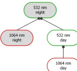
Figure 1. Dependency diagram showing the functional relation-ships between the 532 and 1064 nm CALIOP calibration algo-rithms.
are instead derived from previous calibrations of the 532 nm channel, the uncertainties in the 1064 nm calibration coeffi-cients depend directly on the uncertainties estimated for the 532 nm calibration coefficients. The relationships between the different components of the calibration procedure are di-agramed in Fig. 1. The 1064 nm daytime calibration coeffi-cients are derived from the 532 nm daytime calibration coef-ficients, which in turn are derived from the 532 nm nighttime calibration coefficients (Getzewich et al., 2018). The uncer-tainties for the daytime 1064 nm calibration coefficients thus contain contributions from both the daytime and nighttime 532 nm calibrations.
3 Motivation for change: the V3 calibration algorithms
Effective use of the 1064 nm calibration equation implicitly requires two critically important subroutines:
1. an algorithm to identify cirrus clouds appropriate for use in the calibration calculation and
2. a data averaging scheme to reduce the random noise in the calibration coefficients without simultaneously in-troducing biases.
In this section we review the methods used for these tasks in the CALIOP V3 calibration scheme and point out the short-comings that led to the subsequent development of revised techniques for V4.
3.1 Identifying calibration quality cirrus
As described in H05 and V10, the technique for identifying the calibration targets (i.e., clouds) used in the V3 calibration scheme is straightforward. First, profiles of 532 nm attenu-ated backscatter coefficients,β5320 (z), are averaged horizon-tally and then converted to profiles of attenuated scattering
ratios,R0532(z), where
Rλ0(z)=
βλ,m(z)+βλ,p(z)Tλ,2m(z) Tλ,2O3(z) T
2η λ,p(z)
βλ,m(z) Tλ,2m(z) Tλ,2O3(z)
=
1+ βλ,p(z) βλ,m(z)
Tλ,2ηp(z) . (7) The numerator of Eq. (7) represents the measured attenuated backscatter coefficients, whereβλ,x(z) is a backscatter co-efficient measured for constituentx at altitudezand wave-lengthλ. The constituent-specific attenuations are given by the two-way transmittance terms,
Tλ,x2η(z)=exp
−2ηλ,x z Z
z0
σλ,x(r)dr
, (8)
whereσλ,x(z)is an extinction coefficient andηλ,xis a layer-effective multiple scattering factor. The subscripts O3and m
indicate contributions from, respectively, ozone absorption and molecular backscatter and attenuation, andηm=ηO3= 1 (Winker, 2003; Young and Vaughan, 2009). The quanti-ties in the denominator of Eq. (7) are derived from meteo-rological model data (i.e., profiles of molecular and ozone number densities) obtained from the GMAO. Nighttime pro-files ofR0532(z)are averaged over 15 consecutive laser pulses (∼5 km along track). To reduce the additional noise intro-duced by solar background signals, daytime profiles are aver-aged over 30 consecutive laser pulses (∼10 km along track). These attenuated scattering ratio profiles are then searched downward over an altitude range from 17 to 8.2 km in or-der to identify the highest altitude for whichR5320 (z) >50 for three or more consecutive range bins. All regions satis-fying this search criterion are identified as calibration qual-ity clouds and subsequently used in the V3 1064 nm calibra-tion calculacalibra-tions. Requiring the scattering ratio to exceed 50 throughout the layer minimizes calibration biases by ensur-ing that the molecular contributions to the total backscatter signals will be negligible (see Sect. 7 in H05). On the other hand, the V3 L1 requirements for identifying a layer are very different from those used in the V3 level 2 (L2) analysis, and hence V3 calibration quality clouds typically appear as strongly scattering regions embedded within the more verti-cally extensive structures reported in the V3 L2 data prod-ucts.
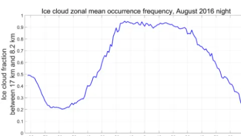
Figure 2.Zonal mean occurrence frequency of ice clouds for V4 nighttime data acquired during August 2016. The solid gray line shows the mean tropopause heights for the month, while the red dashed lines demarcate the V3 calibration cloud search region be-tween 17 and 8.2 km. Polar stratospheric clouds are responsible for the high occurrence frequencies above the tropopause poleward of
∼60◦S.
Figure 3.Latitudinally varying fraction of ice cloud range bins in Fig. 2 that lie within the V3 calibration cloud search limits.
night in the V4 level 2 data during August 2016. Between ∼20◦S and ∼30◦N, the predefined V3 search limits en-compass∼90 % of all range bins classified as containing ice. However, as seen in Fig. 3, outside of this latitude range, the fraction of ice clouds falling with the V3 search limits drops linearly, falling to less than 50 % at ∼34◦S and ∼54◦N. Between ∼70 and∼50◦S, approximately 75 % of the po-tential calibration quality clouds – i.e., tropospheric cirrus – are located below the minimum search altitude of 8.2 km. Based solely on Fig. 3, the fraction of clouds available as po-tential calibration targets appears to increase to∼50 % pole-ward of ∼70◦S. However, Fig. 2 shows that this apparent increase is illusory, as this region is dominated by PSCs that lie well above the local tropopause altitude. The particle sizes in PSCs are often substantially smaller than is typical for tro-pospheric cirrus (Reichardt et al., 2004; Heymsfield et al., 2014), and thus the requisite assumption thatχcirrus≈1
can-not be confidently applied for these layers.
The V3 calibration cloud identification scheme relies solely on the magnitude of the attenuated scattering ra-tios within a fixed altitude range and does not consider other available information such as volume depolarization ratios and/or in-cloud temperatures. One consequence of this choice is the introduction of the second of the three kinds of sampling bias:∼13 % of the clouds used in the V3 calibra-tion scheme are almost certainly water, not ice. This is illus-trated by Figure 4a, which shows the occurrence frequency of the layer-integrated volume depolarization ratios,δv, for
all V3 calibration clouds identified during August 2013. The distribution is clearly bimodal, with a primary peak at δv≈0.39, consistent with cirrus cloud depolarization (Sassen
et al., 2012), and a secondary peak atδv≈0.10, consistent
with the multiple-scattering-induced depolarization observed by CALIOP in dense water clouds (Hu, 2007). Figure 4b shows the distribution ofδvas a function of meanR5320 for
the same V3 calibration clouds. Depolarization ratios below 0.2 are seen to increase approximately linearly as a function of R5320 , as is expected for increasingly dense liquid water clouds (Hu, 2007). On the other hand, there is no obvious trend for those clouds having δv>∼0.3. Figure 4c shows
the distribution ofδvas a function of mid-layer temperature
(Tmid). The depolarization ratios less than 0.2 are strongly
as-sociated with warmer temperatures, giving further credence to the supposition that these clouds are supercooled water clouds.
The third type of bias occasioned by the V3 calibration routine is the risk of differential attenuation of the 532 and 1064 nm signals. WhileX5320 andX10640 are both corrected for wavelength-dependent attenuation effects due to molecu-lar and ozone two-way transmittances, at this initial stage of the lidar data analysis, no correction is possible for as-yet un-detected particulates (i.e., cloud or aerosol layers) lying be-tween the lidar and the top of the calibration cloud. A more rigorous expansion of Eq. (2) would explicitly include these terms; i.e.,
FV3=χcirrus−1
Tp2,1064 0, r ztop X10640 r ztop, r (zbase) T2
p,532 0, r ztop X 0 532 r ztop
, r (zbase)
!
, (9)
where Tp2,λ 0, r ztop represents the particulate two-way
transmittance between the lidar (at range=0) and the top of the calibration cloud (at range=ztop), and the
mean signals are now explicitly calculated over the range from ztop to zbase. The ubiquitous presence of
strato-spheric aerosols suggests that, because the stratostrato-spheric extinction and aerosol optical depth (AOD) are typically larger at 532 than at 1064 nm (Thomason and Peter, 2006), FV3 is slightly overestimated because, in general,
T2p,1064 0, r ztop/T2p,532 0, r ztop>1. For the most
part, this kind of bias error is negligible. However, on those occasions when substantial aerosol or PSC layers are located above a V3 calibration cloud, the resulting biases in FV3
Figure 4.Panel(a)shows the occurrence frequencies of layer-integrated volume depolarization ratios for all calibration clouds identified by the V3 algorithm during August 2013, panel(b)shows the joint distribution of layer-integrated volume depolarization ratios and layer mean attenuated scattering ratio, and panel(c)shows the joint distribution of layer-integrated volume depolarization ratios and mid-layer temperatures. The colors in panels(b)and(c)indicate log10of the number of samples per bin.
the tops of clouds located below the Black Saturday smoke plumes over Australia in February 2009).
3.2 The V3 calibration averaging scheme
Although individual estimates of FV3 use high SNR
mea-surements (i.e.,R5320 (z) >50), the uncertainties for these es-timates are still large, and thus obtaining reliable values re-quires some amount of signal averaging. To maximize the number ofFV3samples averaged, the V3 scheme computes
mean values ofFV3, denoted ashFV3i, over eachgranuleof the CALIOP data record (H05, V10). CALIOP data granules extend from one terminator to the next, thus dividing each or-bit into separate daytime and nighttime segments. This aver-aging scheme implicitly assumes that the pattern of thermally driven intra-orbit changes observed in the 532 nm calibration coefficients (P09) is reproduced more or less identically in the 1064 nm calibration coefficients, and henceFV3can be
considered constant with respect to the elapsed time through-out the individual daytime and nighttime segments of any or-bit. The time-varying V3 1064 nm calibration coefficients are then computed usingC1064(t )= hFV3iC532(t ), wheret
rep-resents granule elapsed time andC532(t) is the 532 nm
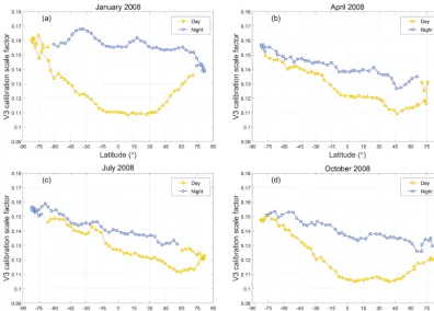
cali-bration coefficient at timet. As illustrated in Fig. 5, monthly averages of instantaneous estimates of FV3, computed as
functions of granule elapsed time and plotted as functions of latitude, demonstrate conclusively that the assumption that
FV3is constant within a granule is not valid.FV3is seen to exhibit a strong dependence on granule elapsed time and can vary by up to 40 % or more within a single granule. Further-more,FV3exhibits a seasonally varying hysteresis, with
lati-tudinal day–night differences being maximized in the boreal winter (Fig. 5a) and minimized during the boreal summer (Fig. 5c).
While the underlying causes of the time-varying behaviors ofFV3have not yet been determined, accurately
compensat-ing for these changes remains essential for reliably calibrat-ing the CALIOP 1064 nm measurements. Reviscalibrat-ing the aver-aging scheme to compute running averages ofFV3as a
func-tion of granule elapsed time would seem to be an obvious strategy for characterizing the intra-orbit changes observed in Fig. 5. However, successful application of this approach on a single granule basis is unlikely simply because the oc-currence of a sufficient number of calibration quality clouds at any location or within any time frame cannot be guaran-teed.
Figure 6 (from Vaughan et al., 2012) shows the monthly occurrence frequency of V3 calibration quality clouds detected during daytime granules as a function of granule elapsed time (y axis) for each calendar month from June 2006 through December 2010 (xaxis). The white grid cells seen along the top edge of the figure represent re-gions where no suitable clouds were detected for the entire month. The sample counts throughout the tropics (i.e., the oscillating dark red region between elapsed times of∼1100 to∼2100 s) are always quite high, and hence estimates of
FV3 can be readily obtained in this region. However,
sam-ple counts in the Arctic (elapsed time > 2500 s) during spring 2008 or late winter 2009 are extremely low, and the likeli-hood of obtaining trustworthy estimates ofFV3in these times
and places is likewise extremely low. Clearly then, any new averaging scheme devised for the V4 calibration must simul-taneously accomplish two tasks. First, it must characterize the calibration scale factors as a function of granule elapsed time throughout the full extent of each granule. And sec-ond, in order to produce high SNR estimates of these time-varying scale factors, the new averaging scheme, in concert with the revised cloud selection routine, must harvest signif-icantly more calibration quality clouds at all latitudes than would be available using the V3 algorithm.
3.3 Calculating profiles of V3 attenuated backscatter coefficients
Once hFV3i has been computed for a granule, the V3
Figure 5.Monthly averages of daytime (yellow) and nighttime (blue) V3 calibration scale factors (i.e.,FV3) as computed as functions of granule elapsed time and plotted as functions of latitude for(a)January,(b)April,(c)July, and(d)October 2008.
Figure 6.Monthly counts of V3 daytime scale factor calculations as a function mission elapsed time (xaxis) and granule elapsed time (yaxis). Colors are displayed on a log10 scale, so that dark reds indicate many thousands of samples, whereas dark blues indicate one or two samples. Regions where no calibration quality clouds were detected are shown in white.
the CALIPSO lidar level 1 data products are then derived as follows (H05):
β10640 (z)=r(z) 2 P
1064(z)−P1064,bkg
G1064E1064C1064
(10) = β1064,m(z)+β1064,p(z)
Tλ,2m(z) Tλ,2O3(z) Tλ,2ηp(z) ,
whereP1064(z) is the backscattered signal from altitude z
measured aboard the satellite in the 1064 nm receiver (units: digitizer counts), P1064,bkg is the background signal
mea-sured aboard the satellite for each profile, and r(z) is the range (units: km) from the lidar to altitudez.E1064 is the
per-pulse energy transmitted at 1064 nm (units: J) and G1064
quantifies the electronic gain at 1064 nm (unitless). The sub-scripts m, p, and O3once again indicate contributions from,
respectively, molecules, particulates, and ozone. The units of β10640 (z)are km−1sr−1. The units of C1064 are km3sr J−1
counts.
4 The version 4 calibration algorithms
Ad-ditionally, we incorporate a seemingly small, but nonethe-less important, change in the way the V4 calibration scale factors, FV4, are calculated. The same calibration transfer
equation still applies; i.e., C1064=FV4C532, as in Eq. (1).
However, in computing FV4, the layer-mean values of the
background-subtracted, range-corrected, gain- and energy-normalized measured backscatter signals,
Xλ0(z)
, are re-placed with the integrated values,Gλ, where
Gλ= base Z
top
X0λ(r)dr−dGλ,where dGλ
=1
2 ztop−zbase
X0λ(zbase)+X0λ ztop, (11)
(e.g., as derived in Eqs. 18–20 in V10), and thus
FV4=χcirrus−1 G
1064 G532
. (12)
The dGλterms represent corrections for the molecular scat-tering contributions to the signals measured within the cloud boundaries. As explained in detail in Sect. 4.1, the V4 cirrus cloud selection method no longer enforces the large scatter-ing ratio requirement (R5320 > 50) that allowed us to neglect these contributions in V3, and thus corrections for molecu-lar scattering are essential in the V4 calibration algorithm. Note, though, that the correction is only applied at 532 nm. Because CALIOP is largely insensitive to molecular scatter-ing at 1064 nm, dG1064is set uniformly to zero.
4.1 Selecting calibration quality cirrus clouds
The selection of calibration quality clouds in V3 was based on two globally applied criteria: layer altitude and the mag-nitude of R0532(z). In contrast, the V4 algorithm identifies calibration quality clouds based on four different quantities: layer altitude, mid-layer temperature (Tmid), layer-integrated
volume depolarization (δv), and layer-integrated attenuated
backscatter at 532 nm (γ5320 ). These latter two quantities are defined as, respectively,
δv= base
P
j=top
X⊥ zj
base P
j=top
Xk zj
, (13)
whereX⊥(z)andXk(z)are, respectively, the signals mea-sured at altitudezin the 532 nm perpendicular and parallel channels, and
γλ0= Gλ Cλ
= zbase
Z
ztop
βλ0(r)dr−dβλ0, (14)
whereβλ0(z)is the attenuated backscatter coefficient at alti-tudezand wavelengthλand dβ0λ=dGλ/ Cλ.
4.1.1 V4 layer detection and selection based on altitude
The V3 calibration algorithm implemented a dedicated layer detection scheme that was sensitive only to strongly scatter-ing features. Moreover, as discussed in Sect. 3.1, the fixed altitude range over which this layer detection procedure was applied effectively eliminated a large fraction of potential calibration quality clouds while at the same time permitting the inclusion of PSCs, for which the assumption ofχcirrus≈1
is not well founded (Sect. 3.1). V4 addresses these defects in two ways. In the most far-reaching change, V4 abandons the dedicated layer detection scheme used in V3 and replaces it with the same layer detection algorithm that is used in the CALIOP L2 analyses (Vaughan et al., 2009). The L2 layer detection algorithm identifies layers having a much wider range of backscatter intensity, and its cirrus detection capa-bilities have been extensively validated (McGill et al., 2007; Thorsen et al., 2011; Yorks et al., 2011; Candlish et al., 2013; Kim et al., 2014). In its standard configuration, the L2 layer detection algorithm applies a nested, multi-resolution data averaging scheme that detects layers at five different hori-zontal averaging resolutions: 1 / 3 km (i.e., single-shot reso-lution), 1, 5, 20, and 80 km. In the 1064 nm calibration algo-rithm, only the 5 km resolution is used, and thus, unlike V3, the profiles ofR5320 (z)used in the V4 layer detection algo-rithm are averaged uniformly over 15 consecutive shots for both daytime and nighttime analyses. These 5 km averaged profiles are then scanned between 30 km and the local sur-face altitude obtained from a digital elevation model (DEM) (Tanelli et al., 2014). Only the uppermost layer detected is further evaluated as a potential calibration quality cloud; lay-ers detected at lower altitudes are discarded, irrespective of their scattering intensity. Enforcing this condition contributes to reducing the severity of the bias errors that can creep into the calculation ofFV4.
The second altitude-based change to the layer acceptance criteria is that the cirrus selection region is no longer static. Instead, within each 5 km horizontal average, a valid cirrus acceptance region is dynamically defined based on maxi-mum altitudes of the local tropopause (obtained from GMAO atmospheric model data) and the Earth’s surface (obtained from a DEM). To account for overshooting cloud tops and uncertainties in the tropopause height, the search for calibra-tion quality clouds begins 2 km above the maximum GMAO tropopause altitude. Similarly, to eliminate the possibility of surface contamination, the search is terminated 1 km above the maximum DEM altitude.
cloud was used to calculate estimates ofFV3in the V3 data
set. But because smoke is strongly absorbing at 532 nm, with Ångström exponents typically in the neighborhood of 1.8– 2.0 (Chand et al., 2006, 2008), the differential attenuation term in Eq. (9) becomes notably larger than 1, and the esti-mates ofFV3are biased correspondingly high. This is not an
issue in V4. The cirrus layer will not be considered for the calibration routine, simply because it is not the highest layer detected in the profile. And while the smoke layer is consid-ered, it is subsequently rejected based on additional criteria described in the following sections.
4.1.2 Selection based onTmidandδv
In deriving a more comprehensive set of selection crite-ria for identifying calibration quality clouds, our initial ef-forts focused on determining appropriate thresholds for mid-layer temperature and mid-layer-integrated depolarization ratio. To test the proposition that supercooled water clouds (e.g., as in Fig. 4) were biasing calculations ofFV3, we generated
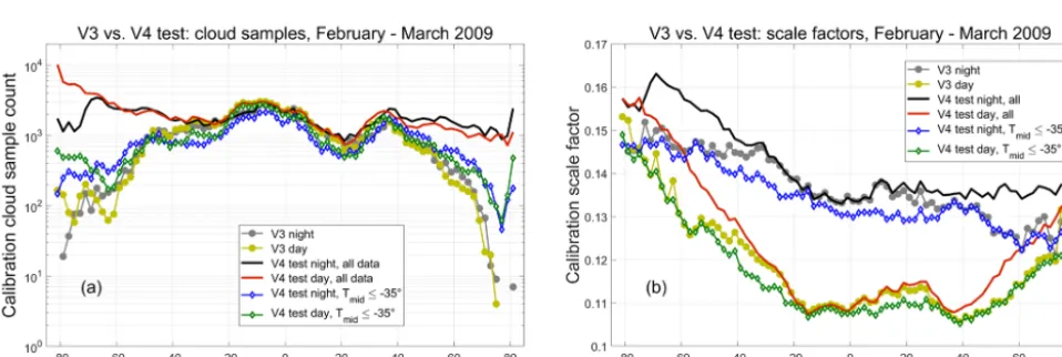
2 months of test data (February and March 2009) for which the layer search region was defined by the local tropopause and DEM surface (see Sect. 4.1.1), but the sole layer selec-tion criterion remained, as in V3, R0532> 50 for three con-secutive range bins. As expected, changing the search region greatly increased the number of calibration quality clouds de-tected at higher latitudes (red and black lines in Fig. 8a). At the same time, this change also greatly increased both the mean magnitude of the calibration scale factors computed poleward of ±30◦ (red and black lines in Fig. 8b) and the variability of the calibration scale factors computed in these regions. This increase in magnitude and variability is caused by the much wider range of mid-cloud temperatures in the lower-altitude data set. When the test data are restricted to calibration clouds with mid-layer temperatures of−35◦C or colder (blue and green lines in Fig. 8), the number of samples poleward of±30◦ falls by an order of magnitude or more, and the scale factors drop to levels similar to those in the V3 data. Figure 9a shows the distribution of the scale factors as a function of mid-layer temperature. The scale factors appear to be naturally partitioned into two clusters that fall on either side of a dividing line at−35◦C, with the colder clouds hav-ing a lower mean scale factor and showhav-ing less variability.
As seen in Fig. 9b, the 532 nm layer-integrated volume depolarization ratios also appear to cluster into two distinct groups, with centers falling on either side of a dividing line atδv=0.3. Figure 9c plots the occurrence frequency ofδv
as a function of Tmid, and shows a structure that is
essen-tially identical to what is seen in Fig. 4c. The dividing lines at Tmid= −35◦C and δv=0.3 partition the data into four
quadrants. The upper left quadrant, where Tmid<−35◦C
andδv> 0.3, can be confidently assumed to contain only ice
clouds (Campbell et al., 2015). The bottom right quadrant is, in all likelihood, populated mostly by supercooled water clouds. Table 1 shows the descriptive statistics for the scale
Table 1.Descriptive statistics for the scale factors associated with the data points in the upper left and lower right quadrants of the right panel in Fig. 9 (MAD: median absolute deviation).
Tmid<−35◦C Tmid>−35◦C andδv> 0.3 andδv< 0.3
Minimum 0.0174 0.0783
Maximum 0.2268 0.3979
Median 0.1270 0.1482
MAD 0.0129 0.0159
Mean 0.1262 0.1498
Standard deviation 0.0160 0.0214
Samples 104 728 117 176
factors associated with the data points in the upper left and lower right quadrants of Fig. 9c. In the mean, the scale fac-tors in the upper left quadrant are smaller than those in the lower right quadrant by∼19 %.
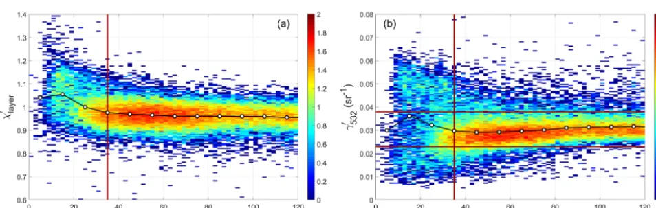
4.1.3 Selection based onγ5320
The fundamental assumption underlying the CALIOP 1064 nm calibration scheme is that, because the ice crys-tals in cirrus clouds are most often quite large relative to the CALIOP wavelengths, the layer-mean cirrus backscatter coefficients are spectrally independent at 532 and 1064 nm (Reagan et al., 2002). Satisfying this assumption thus re-quires some method for estimating cirrus particle size prior to calibrating the 1064 nm channel. To accomplish this, we used the CALIPSO V3 level 2 lidar and IIR track data products to derive an empirical relationship betweenγ5320 , which is read-ily obtained from the calibrated 532 nm measurements, and the effective diameters retrieved from exactly collocated IIR measurements (Garnier et al., 2012, 2013). Figure 10 com-pares the lidar measurements to the collocated IIR retrievals for all clouds used in the V3 1064 nm calibration scheme during October 2010. As seen in Fig. 10a, the V3 attenu-ated backscatter color ratios,χlayer0 =γ10640 /γ5320 , remain rel-atively constant for IIR effective diameters above∼35 µm, with a mean value of 0.96±0.05. Similarly, Fig. 10b shows that the majority of these large effective diameters are con-centrated within aγ5320 range between 0.023 and 0.038 sr−1.
Figure 7. (a)CALIOP 532 nm attenuated backscatter coefficients (km−1sr−1) showing smoke from the February 2009 Black Saturday fires in Australia lofted over an opaque cirrus deck;(b)a profile of attenuated scattering ratios (in green) for which the cirrus beneath the smoke plume qualifies as a calibration quality cloud in the V3 algorithm. In panel(b), the blue dashed vertical line indicates an attenuated scattering ratio of 1, while the red dashed vertical line indicates the V3 cloud detection threshold ofR5320 =50. Below the high-altitude smoke plume, the ratio of particulate two-way transmittances is T2p,1064/Tp2,532=1.25±0.20.
Figure 8. (a)Sample counts and(b)mean scale factors for all daytime and nighttime granules acquired during February and March 2009. V3 results are shown in yellow (day) and dark gray (night). The initial test results (new altitude regime only) are shown in red (day) and black (night). The test results with a−35◦C temperature requirement imposed are shown in green (day) and blue (night).
In addition to identifying clouds comprised of large par-ticles, the V4 calibration cloud selection scheme must also ensure that these large particles are ice. For CALIOP, cloud ice–water phase is readily determined by the relationship be-tween γ5320 and δv (Hu, 2007; Hu et al., 2009). Figure 11
shows the joint occurrence frequencies ofδvandγ5320 for
dif-ferent subsets of clouds detected during October 2010. Fig-ure 11a shows data from only those clouds that were de-tected at a 5 km horizontal resolution and were the highest cloud detected in each profile. Randomly oriented ice (ROI) clouds are characterized by smaller integrated attenuated backscatters and higher depolarization ratios, withδvfor ice
clouds being largely independent of γ5320 . Water clouds, on the other hand, generally have much larger integrated
atten-uated backscatter coefficients, and there is a strong linear re-lationship between the magnitudes ofδvandγ5320 . The small
population of clouds dominated by horizontally oriented ice (HOI) crystals, shown in the bottom right of Fig. 11a, has very largeγ5320 andδvclose to zero. Figure 11b showsδvand
γ5320 calculated over the full vertical extent of all calibration quality clouds identified by the V3 1064 nm calibration algo-rithm. As seen below the solid orange line in Fig. 11b, the V3 1064 nm calibration coefficients for October 2010 are bi-ased by the inadvertent inclusion of a non-negligible fraction of water clouds.
Figure 9.For the February and March 2009 test data set, panel(a)shows the occurrence frequency ofFV3as a function of mid-layer temperature, panel(b)shows the occurrence frequency ofFV3as a function of 532 nm layer-integrated volume depolarization ratio, and panel(c)shows the occurrence frequency of layer-integrated depolarization as a function of mid-layer temperature. For all panels, the plot colors represent log10of the number of sample counts in each grid cell.
Figure 10. (a)χlayer0 and(b)γ5320 as functions of IIR-derived effective particle size for all nighttime calibration quality clouds detected by the V3 1064 nm calibration scheme during October 2010. The filled circles in each panel represent median values of the distributions. The horizontal red lines in panel(b)showγ5320 limits of 0.023 sr−1(lower line) and 0.038 sr−1(upper line).
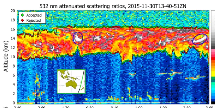
due to molecular contributions to the total scattering from the clouds. In V4 this scattering intensity criterion is satisfied us-ingγ5320 , with the contributions from molecular scattering be-ing accounted for by the dG532term in Eq. (11). An example of the differences in calibration cloud sample sizes associated with these two metrics is illustrated in Fig. 12. The V3 cal-ibration analysis identified seven calcal-ibration quality clouds in this scene, shown as intermittent occurrences within the brightest white regions circled in blue between 12 and 14 km and clustered near 1.2◦N and 3.4◦S. Clearly these V3 cal-ibration quality clouds would more accurately be described as “cloud fragments”, as those regions for which three con-tiguous bins ofR0532(z)exceed 50 typically represent only a small fraction of the full vertical extent of the cloud identi-fied by the L2 layer detection scheme. Of the 160 layers de-tected at 5 km horizontal resolution by the V4 analysis, 116 had 532 nm integrated attenuated backscatters in the accept-able range of 0.023 sr−1<γ5320 < 0.038 sr−1, amounting to a 22-fold increase in the number of potential calibration qual-ity clouds.
4.1.4 Comprehensive selection strategy implemented in V4
Summarizing the criteria described in the previous subsec-tions, clouds selected for use in the V4 1064 nm calibration algorithm are detected using the same layer detection algo-rithm that is used in the CALIOP level 2 analyses and are required to meet all of the following specifications.
(a) The cloud must be the uppermost layer detected in a profile averaged to a 5 km horizontal resolution (Sect. 4.1.1).
(b) The boundaries and vertical extent of this uppermost layer are constrained by the local tropopause height at the upper end and the Earth’s surface at the lower end (Sect. 4.1.1).
(c) The temperature at the cloud geometric midpoint must be colder than−35◦C (Sect. 4.1.2).
Figure 11.Panel(a)shows the joint occurrence frequency ofδvandγ5320 for clouds measured by CALIOP during October 2010. Only layers detected at 5 km horizontal resolution that are the uppermost layer in each profile are included. The solid black line differentiates randomly oriented ice clouds (above the line) from water clouds (below the line). Clouds containing horizontally oriented ice crystals occur within the oval at the bottom of the plot. Panel(b)shows the joint occurrence frequency ofδvandγ5320 for clouds used in the V3 1064 nm calibration analysis. The population of points below the orange threshold line quantifies the occurrence frequency of water clouds in the October 2010 V3 calibration data set. In both plots, the colors indicate log10of the number of samples in each grid cell.
Figure 12.532 nm attenuated scattering ratios, averaged to 5 km horizontally and 60 m vertically, for an extended cirrus layer in the southwest Pacific near New Caledonia on 30 November 2015. Potential V3 calibration opportunities (R0532> 50) in the cirrus layer are shown as bright white patches lying within the blue ovals. V4 cloud boundaries are indicated by filled diamonds. The boundaries of those clouds for which 0.023 sr−1<γ5320 < 0.038 sr−1are shown in green. The boundaries of clouds havingγ5320 outside this range are shown in red.
for the lower limit is described in Sect. 4.1.2. The upper limit is defined to eliminate unusually large noise excur-sions that can occur during daytime measurements of cirrus above bright clouds or desert surfaces or during both daytime and nighttime when transiting the South Atlantic Anomaly (SAA; see Noel et al., 2014). (e) The layer-integrated 532 nm attenuated backscatter is
restricted to a range of 0.023 sr−1<γ5320 < 0.038 sr−1 (Sect. 4.1.3).
Enforcing these criteria ensures a substantially more ho-mogenous population of clouds than was used in V3. Water clouds are effectively eliminated by theTmidandδv
require-ments, clouds dominated by horizontally oriented ice crystals are rejected by theγ5320 andδvlimits, and polar stratospheric
sam-ples that would have been obtained had the conditions (a) through (e) above been applied instead (Fig. 13b). The V4 selection parameters are seen to provide a much more uni-form sampling as a function of latitude, while at the same time delivering a substantially larger number of total sam-ples (59 675 in V3 vs. 92 132 in V4).
4.2 Characterizing intra-orbit changes using multi-granule data averaging
The primary motivation for the complete redesign of the CALIOP 1064 nm calibration scheme is to accurately charac-terize the time-varying behavior of the calibration scale fac-tors. As illustrated in Fig. 5, these changes occur on mul-tiple timescales, from intra-orbit to seasonal. Designing an effective data averaging scheme thus becomes a question of balancing requirements in two time dimensions: along track within a single granule and again across multiple gran-ules. Specifically, we need to accumulate a sample size large enough to minimize the random uncertainty in our estimates ofFV4, while at the same time (a) limiting the extent of the
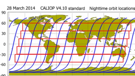
along-track averaging in order to reliably capture the depen-dence of scale factors with respect to granule elapsed time and (b) limiting the duration of our multi-granule averag-ing window to prevent smearaverag-ing of legitimate changes in the scale factors that occur on weekly-to-seasonal timescales. The (not-to-scale) dimensions of the averaging window de-veloped for the V4 1064 nm calibration scheme are illus-trated in Fig. 14. The red boxes indicate notional averaging regions that extend both along track (i.e., north–south within any one granule) and across-track (i.e., in the east–west di-rection, spanning multiple granules).
The driving factor in sizing this two-dimensional averag-ing window is the number of calibration quality clouds that can be measured in the cloud-sparse seasons and regions of the planet. For the V3 calibration procedure, these regions are indicated by the white grid cells shown in Fig. 6. But be-cause V4 uses entirely different cloud selection criteria, the cloud-sparse seasons and regions of the planet are also quite different. Figure 15 shows V4 calibration cloud occurrence frequency as a function of granule elapsed time in increments of 90 s (equivalent to an along-track averaging distance of ∼605 km) for the months of January, April, July, and Octo-ber 2014. For nighttime data (Fig. 15a), granule elapsed time begins at the day-to-night terminator in the Northern Hemi-sphere and tracks the temporal progress of the descending node of each orbit. Granule elapsed time for daytime data (Fig. 15b) begins in the Southern Hemisphere and tracks the ascending node of each orbit. For the nighttime data, a min-imum value of 276 calibration quality clouds occurs during July at a median granule elapsed time of 1215 s (equivalent to∼15◦S). For the daytime data, a minimum value of 342 calibration quality clouds occurs during January at a median granule elapsed time of 495 s (equivalent to∼80◦S on the ascending node). Given that the random relative uncertainty
in CALIOP’s assumed value ofχcirrusis±0.25 (Vaughan et
al., 2010), reducing this uncertainty by a factor of 10 requires averaging 100 or more independent samples. In the V4 cali-bration procedure we achieve this goal at an along-track tem-poral resolution of 90 s by using a fixed 7-day averaging win-dow, encompassing a maximum of 105 granules, centered about the current orbit location (i.e.,∼ ±54 granules from the current granule). This strategy typically yields well over 250 samples per average, though, as demonstrated in Fig. 15, the total for any average varies by both season and location. These averaging intervals are uniformly applied whenever the instrument is in continuous data acquisition mode. As discussed in Getzewich et al. (2018), interruptions (e.g., for periodic boresight alignments, as described in Hunt et al., 2009) require a reboot of the calibration procedures at both wavelengths. When these reboots occur, the data averaging intervals are reinitiated. For a variety of reasons, the cali-bration coefficients and scale factors can be notably differ-ent immediately before and after an interruption (Getzewich et al., 2018). Section 4.3.2 discusses some consequences of these reboots that are specific to the 1064 nm calibration pro-cedures.
4.3 Uncertainty estimates
The calibration coefficients estimated by CALIOP 1064 nm calibration algorithm are subject to both random uncertain-ties, which can be substantially reduced by applying the ap-propriate averaging techniques, and systematic bias error, which cannot be reduced by averaging. The sections below discuss both types of errors and describe how input uncer-tainties propagate into the final values of the 1064 nm cali-bration coefficients.
4.3.1 Random uncertainties
The random uncertainties in the V4 calibration coefficients are derived using the same formalism used in V3, but with
Gλreplacing
X0λ(r); i.e.,
1C1064 C1064 2 = 1fV4 fV4 2 + 1C532 C532 2 = 1χcirrus χcirrus 2 +
1G1064
G1064
2 +
1G532
G532 2 + 1C532 C532 2 , (15)
where1C532and1FV4depend critically on the amount of
averaging done when deriving the required estimates ofC532
andFV4. Nighttime and daytime derivations for1C532/C532
are given in, respectively, Kar et al. (2018) and Getzewich et al. (2018). Random uncertainties for the 532 nm calibra-tion coefficients are typically on the order of 1.5 % or less, both at night and during the day. The multi-granule moving window averaging scheme described in Sect. 4.2 is specif-ically designed to minimize random uncertainties in FV4.
Figure 13. (a)γ5320 for all V3 calibration clouds as a function of latitude, and(b)γ5320 for all V4 calibration clouds as a function of latitude for October 2010 nighttime measurements. The filled circles in each plot representγ5320 mean values over 2◦latitude increments; error bars indicate±1 SD about the means. The colors indicate log10of the number of samples in each grid cell.
Figure 14. Nighttime orbit tracks for 28 March 2014 (in blue), overlaid with notional averaging domains (red boxes) that extend over two time dimensions; i.e., traveling along track (north–south) within individual granules, and spanning the same along-track dis-tance across multiple granules (east–west).
and standard deviations for the calibration scale factors ac-quired over 90 s intervals of granule elapsed time during the 7-day period from 24 to 30 November 2015. Figure 16b shows the number of samples acquired in each 90 s time bin. The minimum sample count is 317, occurring at ∼81.7◦S during the daytime. The relative uncertainties in the mean values of FV4 in each 90 s interval (i.e., standard devia-tion/(mean×√sample counts)) range between 0.11 % and 0.40 % at night (mean: 0.22 %±0.07 %) and 0.17 % and 0.52 % during the day (mean: 0.29 %±0.09 %). Sinceχcirrus
is a constant for all calculations, these uncertainties quan-tify the random variability in the G1064/G532 term of FV4.
But by averaging many samples we also reduce the random uncertainty in our estimate ofχcirrus. In this example, the
rel-ative uncertainty attributed toχcirrusis reduced from a single
sample value of∼25 % to mean values of 0.93 %±0.20 % during the day and 0.97 %±0.24 % at night. Both in this
ex-ample and throughout the entire V4 data set,χcirrusremains
the dominant random uncertainty in estimatingFV4.
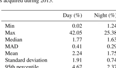
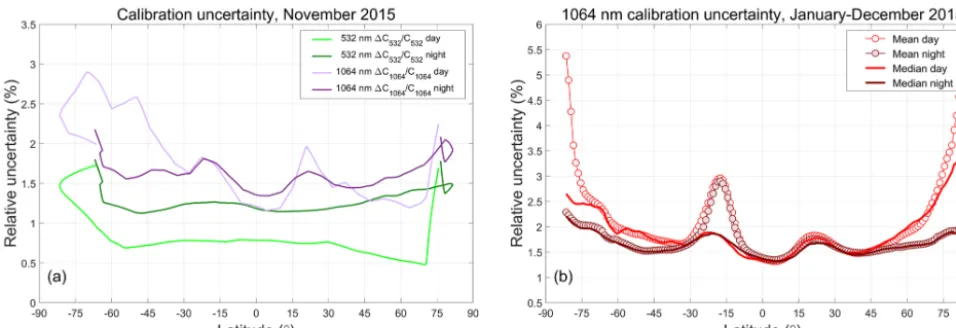
The CALIOP V4 data products report estimates of ran-dom uncertainties in the 532 and 1064 nm calibration co-efficients on a profile-by-profile basis. Figure 17a plots the mean values of the relative calibration coefficient uncertain-ties at both wavelengths as functions of latitude for all of November 2015. The dip in sample counts shown at∼20◦N in the right-hand panel of Fig. 16 is echoed by the increase in 1064 nm calibration uncertainty seen at the same lati-tude in Fig. 17. The mean and median relative uncertain-ties for all 1064 nm calibration coefficients computed from 1 January through 31 December 2015 are shown in Fig. 17b and further summarized in Table 2. Taken over the full year and the full globe, the median relative uncertainties during the daytime are 1.77 %±0.41 %. Nighttime uncertainties are slightly lower, at 1.63 %±0.29 %. Median uncertainties re-main below 2 % daytime and nighttime between∼60◦S and ∼60◦N. The largest relative uncertainties occur in the SAA and for daytime measurements in the polar summers. In po-lar summers, the daytime 532 nm calibration coefficients and uncertainties cannot be calculated directly but instead are interpolated between the last known-to-be-valid calibration coefficients in the daytime portion of the orbit and the first last known-to-be-valid calibration coefficients in the night-time portion of the same orbit (see Fig. 4 and Sect. 3.7 in Getzewich et al., 2018).
4.3.2 Bias errors
cal-Figure 15.V4 calibration cloud occurrence frequency as a function of granule elapsed time (90 s bins) for January, April, July, and Octo-ber 2014. Panels(a)and(b)show, respectively, nighttime data and daytime data.
Figure 16. (a)mean values (filled circles) and single-sample standard deviations (error bars) for the calibration scale factors averaged over 90 s intervals during the 7-day period from 24 to 30 November 2015;(b) the number of calibration quality clouds sampled in each 90 s interval.
Table 2.Summary of CALIOP V4 single-profile relative calibra-tion coefficient uncertainties for all 1064 nm attenuated backscatter profiles acquired during 2015.
Day (%) Night (%)
Min 0.02 1.24
Max 42.05 25.38
Median 1.77 1.63
MAD 0.41 0.29
Mean 2.24 1.75
Standard deviation 1.91 0.74
95th percentile 4.67 2.37
Samples 308 277 495 271 947 645
culations. Whenever lidar operations are temporarily halted – e.g., due to space weather anomalies or off-nominal instru-ment behavior – the instruinstru-ment is commanded to safe mode, and the standard operating temperatures within the transmit-ter and receiver are no longer rigorously maintained. When the lidar is subsequently restarted after a long duration outage (e.g., 1 or more days), 36 to 72 h of continuous operation can be required before full thermal stability is reestablished. The detector gains for both the PMTs and the APD are tempera-ture sensitive, so during this warm-up period the calibration coefficients for both channels will approach their steady-state behaviors, though not necessarily at the same rate.
The effects of the changing detector gains during the in-strument warm-up period are illustrated in Fig. 18a, which shows the granule mean of the estimatedχ0,
χ0
Figure 17. (a) Mean relative calibration coefficient uncertainties, daytime and nighttime, at 532 nm (greens) and 1064 nm (purples) for November 2015; (b)mean and median relative calibration uncertainties at 1064 nm for all data acquired during 2015. In(b), the large excursion in the mean uncertainties at∼20◦S is due to increased uncertainties in the 532 nm calibration coefficients due to high radiation noise in the SAA (Hunt et al., 2009; Noel et al., 2014).
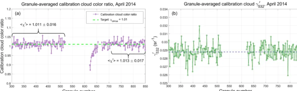
number 301) and 30 April 2014 at 13:21:37 UTC (granule number 849). Due to space weather considerations (i.e., an elevated 10 MeV proton flux), the CALIPSO payload was placed in safe mode at 08:29:42 UTC on 19 April 2014, and no instrument data were collected until the payload was restarted at 16:26:07 UTC on 22 April 2014. Prior to shut down,
χ0
oscillated consistently around the expected value of 1.01. However, when the lidar was restarted, the initial val-ues ofχ0were seen to be substantially lower, though over the course of multiple granules, χ0 gradually and nonlin-early returned to∼1.01. This same behavior is clearly evi-dent in the data acquired following any shutdown of∼12 h or longer.
The exact mechanisms driving this behavior in the calibra-tion cloud color ratios are not yet fully understood. However, as illustrated in Fig. 18b, which shows granule meanγ5320 for the April 2014 time period, the granule meanγ5320 for cali-bration quality clouds is essentially unaffected by the time-varying detector gains. The granule mean γ5320 prior to the data outage (granules 301–519) is 0.0288±0.009 sr−1. Fol-lowing the data outage (granules 619–849), the granule mean γ5320 is essentially unchanged at 0.0289±0.008 sr−1. The variability within this time series can be largely attributed to the natural variability ofγ5320 for individual calibration qual-ity clouds. Given that γ5320 =G532/C532 remains essentially
constant across the data outage, while χ0=γ10640 /γ5320 = G1064/(C1064×γ5320 ) varies, current investigations are
fo-cused on the 1064 nm channel measurements (i.e.,G1064) and possible time-varying biases in the calculation ofC1064.
Potentially biased estimates ofC1064can be identified in
the L1 profiles by examining the “QC_Flag_2” scientific data set (SDS) in the CALIOP level 1b profile products. These QC flags are implemented as 32-bit integers, and interpreted as a series of Boolean values, with each bit indicating a specific
warning or error condition. A QC_Flag_2 of zero indicates that none of these warnings or error conditions has occurred. Those profiles for whichC1064may be biased will have bit 27
toggled on (bit 26 if zero-based indexing is used), and thus an otherwise error-free profile with a possibly biased estimate of C1064will have a QC_Flag_2 of 67 108 864.
Section 4.3.1 demonstrated that χcirrus is the dominant
source of random uncertainties in the 1064 nm calibration scale factor error budget. While the random uncertainties in the calibration scale factors due to χcirrus can be reduced
by averaging,χcirrusis also a potential source of irreducible
bias errors. The best available estimate of the mean value of χcirrus remains 1.01, as determined in V10 and verified by
experimentally by Haarig et al., 2016. However, the uncer-tainty in this estimate is large (±0.25), and the true value of χcirrusmay be somewhat different from the value used in the
CALIOP V4 calibration algorithm (e.g., 1.00 vs. 1.01, which would introduce a bias of 1 % into the scale factor calcula-tions).
5 Performance assessments and comparisons to version 3
Figure 18. (a)Time series of granule meanχ0measured for calibration quality clouds detected during nighttime orbit segments beginning on 11 April 2014 (granule 301), and extending through 30 April 2014 (granule 849). Due to adverse space weather, CALIOP was placed in safe mode, and thus data are missing for over 3 days, from 19 April 2014 at 08:29:42 UTC to 22 April 2014 at 16:26:07 UTC, spanning granules 521–619. A smaller data gap of just over 8 h (from 01:09:36 until 09:38:09 UTC on 24 April 2014, spanning granules 657–669) occurs during a satellite drag make-up maneuver. A distinct drop in the magnitude ofχ0occurs when the lidar is restarted on 22 April. Because there were two instrument shutdowns in relatively rapid succession, full recovery to the pre-outage values takes place over∼72 h.(b)Granule mean γ5320 for the same time period. These values remain relatively constant throughout the entire measurement interval, suggesting that the 532 nm calibration appropriately compensates for any time-dependent detector gain changes following an instrument restart.
5.1 Daily-to-monthly changes
The magnitude and spatial variability of the granule-to-granule changes in the calibration coefficients are illustrated in Fig. 19, which shows maps of the mean V3 and V4 cal-ibration coefficients for daytime (Fig. 19a–c) and nighttime (Fig. 19d–f) calculated for March 2015. In the V3 calibra-tion coefficient images (Fig. 19a and d), individual ule tracks are easily discerned, indicating that these gran-ules have unusually large or unusually small calibration co-efficients relative to neighboring granules. This “striping” of the V3 1064 nm calibration coefficients occurs because a single mean scale factor is calculated for each granule, and thus, when cloud locations or occurrence frequencies shift substantially from one orbit to the next, the concomi-tant changes in the mean scale factor introduce noticeable granule-to-granule discontinuities in the calibration coeffi-cients. Because the V4 algorithm computes scale factors by averaging over multiple granules, corresponding to approxi-mately 1 week of observations, this vertical striping is elim-inated in the V4 images and data (Fig. 19b and e). Addi-tionally, the influence of the SAA, seen in the nighttime data shown in Fig. 19d and f, is now virtually eliminated.
Maps of the monthly mean V3 calibration coefficients di-vided by the monthly mean V4 calibration coefficients are shown in Fig. 19c and f. In this example, the variability be-tween the two data versions extends from −20 % (daytime Southern Hemisphere) to+25 % (nighttime Northern Hemi-sphere). The changes in the daytime range from +20 % in the northern midlatitudes to−20 % in Antarctica. Nighttime changes are somewhat more muted in this example, varying between+25 % in the Arctic to−7 % in Antarctica.
5.2 Day-to-night calibration continuity
An important detail that may not be immediately apparent in Fig. 19 is shown explicitly in Fig. 20, where the March 2015 zonal mean calibration coefficients for both V3 (Fig. 20a) and V4 (Fig. 20b) are plotted separately for daytime and nighttime granules as a function of latitude. The V3 1064 nm calibration coefficients show large discontinuities when the instrument transitions from day to night (Fig. 20a, left side) and again from night to day (Fig. 20a, right side). In contrast, the V4 calibration coefficients show no discontinuities cross-ing the terminators. Because the signals are normalized with respect to electronic gains prior to calibration, this smoothly varying transition across the terminators is the expected be-havior. However, ensuring that the scale factors are contin-uous across the terminators (e.g., as shown in Fig. 16) does not guarantee that the desired outcome actually occurs; the 532 nm calibration coefficients must also be continuous. The substantial changes made in the daytime 532 nm calibration algorithm (Getzewich et al., 2018) are thus an essential pre-condition for achieving the required continuity at 1064 nm. 5.3 Seasonal-to-yearly changes
The seasonal and annual changes between the V3 and V4 nighttime granule-averaged estimates ofC1064are illustrated
Figure 19. V3 and V4 calibration coefficients for March 2015. Panels(a)through(c)show daytime mean 1064 nm calibration coeffi-cients (units: km−3sr J−1count); V3 is shown in panel(a), V4 in panel(b), and their ratios ((V3–V4)/V3) in panel(c). Similarly, panels (d)through(f)show nighttime mean 1064 nm calibration coefficients (units: km−3sr J−1count), with V3 shown in panel(d), V4 in panel (e), and their ratios (V3/V4) in panel(f).
Figure 20.Zonal mean 1064 nm calibration coefficients for March 2015; panel(a)shows V3 calibration coefficients (units: km−3sr J−1), while panel(b)shows the V4 coefficients (units: km−3sr J−1count). In both panels, nighttime values are shown in blue and daytime values in yellow. Error bars represent 1 standard deviation about the mean.
magnitude of the V3 oscillations is significantly amplified by the data averaging strategy implemented in V3 calibra-tion procedure. The left panel of this figure shows the daily mean latitude centroid,
Clatitude= N P
n=1
latituden×FV3n N
P
n=1 FV3n
, (16)
computed over all nighttime scale factors for each calen-dar day for which there were CALIOP measurements dur-ing 2013–2017. This quantity represents the characteristic
latitude associated with the daily mean value ofFV3. The seasonal oscillations ofClatitudereflect changes in the
occur-rence frequencies of strongly scattering
R5320 >50
con-vective ice clouds. As seen in Fig. 22b,FV3is a decreasing
function of latitude, and the scale factors measured in the Southern Hemisphere are systematically higher than those in the Northern Hemisphere. The seasonal shifting ofClatitude
thus introduces seasonal oscillations inFV3 (green line in
Figure 21.Granule-mean calibration coefficients (scaled by 10−9, with units=km−3sr J−1 count) for V3 and V4 from 1 Jan-uary 2013 through 31 December 2017. The large data gap from 28 January through 14 March 2016 is due to a GPS anomaly that interrupted the timekeeping services normally provided by the satel-lite. Adverse space weather is responsible for the smaller gap from 5 through 15 September 2017.
6 Comparisons to other techniques and measurements
While CALIOP uses cirrus clouds to calibrate its 1064 nm measurements, other calibration targets are also available. SNR limitations rule out molecular normalization as an op-tion. However, water clouds and ocean surfaces offer poten-tially attractive alternatives; both are typically measured with very high SNR, and their spectral differences in backscatter are well-characterized by theory. In this section we explore the relative merits of using water clouds and/or ocean sur-faces as 1064 nm calibration targets. Calibration algorithms for both targets are briefly described, and the calibration co-efficients derived using these algorithms are compared to the standard values reported in the CALIOP level 1 data prod-ucts. In addition, we compare CALIOP’s 1064 nm attenu-ated backscatter profiles to coincident attenuattenu-ated backscatter profiles acquired independently by the airborne high spec-tral resolution lidar (HSRL) developed at NASA’s Langley Research Center (LaRC). The results of these studies will al-low us to estimate an upper bound on the bias errors in the CALIOP 1064 nm calibration coefficients.
6.1 Lidar calibration using ocean surfaces
Ocean surfaces have long been proposed as calibration tar-gets for airborne and space-based lidars (Bufton et al., 1983; Menzies et al., 1998; Josset et al., 2010). In particular, Menzies et al. (1998) described a technique for using lidar backscatter measurements of the ocean surface to derive es-timates of 1064 nm calibration coefficients relative to known 532 nm calibration coefficients. Leveraging the ocean surface scattering equations in Venkata and Reagan (2016), we adapt the multiwavelength approach of Menzies et al. (1998) to obtain estimates of the CALIOP 1064 nm calibration
coef-ficients from the following relationship:
C1064=C532
R
f,532
Rf,1064
T2
p,532(0, zsurface)
Tp2,1064(0, zsurface) !
·
tsurfacebase R
tsurfacetop
X01064(t )dt
tsurfacebase R
tsurfacetop
X0532(t )dt
. (17)
In computing these values, the signals are integrated over the time duration of the ocean surface backscatter pulses (i.e., fromtsurfacetop totsurfacebase), which are broadened over mul-tiple time intervals (i.e., range bins) by third-order low-pass Bessel filters in the CALIOP receiver electronics (Hu et al., 2007d; Venkata and Reagan, 2016). TheRf terms are the Fresnel reflectance coefficients of seawater, which we take to be 0.0213 at 532 and 0.0202 at 1064 nm (Quan and Fry, 1995), and the T2 terms represent the two-way attenuation of the signal due to clouds and/or aerosols between the lidar and the ocean surface. By calibrating relative to the 532 nm channel, we eliminate the need for accurate estimates of wind speeds, wave slope variances, and whitecap frequencies that would otherwise be required to directly calibrate the 1064 nm channel using ocean surface measurements (Lancaster et al., 2005).
Equation (17) has the same general form as Eq. (1); that is, the 1064 nm calibration coefficient is obtained by mul-tiplying a previously derived 532 nm calibration coefficient by a (possibly time-varying) scale factor computed based on the differences in backscatter signal magnitudes from some well-characterized target. A 1-month comparison of ocean surface scale factors to the cirrus cloud scale factors used to calibrate the V4 data products is shown in Fig. 23. The ocean data are derived for daytime measurements during the month of October 2010 between 60◦N and 60◦S. The lati-tude limits were enforced to minimize possible sea ice con-tamination of the ocean surface samples. To further reduce the possible inclusion of sea ice samples, the ocean surface depolarization ratios were constrained to lie between 0 and 0.15 (Lu et al., 2017). Ocean surface scale factors were com-puted at single-shot resolution using V4 level 1 profiles in which no clouds were detected in any of the CALIOP level 2 data products. Aerosol loading was minimized by requiring the column-integrated attenuated backscatters at 532 nm to lie between 0.0036 and 0.0176 sr−1. Estimates of the aerosol