go.warwick.ac.uk/lib-publications
Original citation:
Buxton, Samuel and Habershon, Scott. (2017) Accelerated path-integral simulations using
ring-polymer interpolation. Journal of Chemical Physics, 147 . 224107.
Permanent WRAP URL:
http://wrap.warwick.ac.uk/97110
Copyright and reuse:
The Warwick Research Archive Portal (WRAP) makes this work by researchers of the
University of Warwick available open access under the following conditions. Copyright ©
and all moral rights to the version of the paper presented here belong to the individual
author(s) and/or other copyright owners. To the extent reasonable and practicable the
material made available in WRAP has been checked for eligibility before being made
available.
Copies of full items can be used for personal research or study, educational, or not-for profit
purposes without prior permission or charge. Provided that the authors, title and full
bibliographic details are credited, a hyperlink and/or URL is given for the original metadata
page and the content is not changed in any way.
Publisher’s statement:
This article may be downloaded for personal use only. Any other use requires prior
permission of the author and AIP Publishing.
The following article appeared in Buxton, Samuel and Habershon, Scott. (2017) Accelerated
path-integral simulations using ring-polymer interpolation. Journal of Chemical Physics, 147 .
224107. and may be found at
https://doi.org/10.1063/1.5006465
A note on versions:
The version presented here may differ from the published version or, version of record, if
you wish to cite this item you are advised to consult the publisher’s version.
Accelerated path-integral simulations using ring-polymer interpolation
Samuel J. Buxton1and Scott Habershon1,a)Department of Chemistry and Centre for Scientific Computing, University of Warwick, Coventry, CV4 7AL, United Kingdom
Path-integral (PI) molecular simulations can be used to calculate exact quantum statistical mechanical prop-erties for complex systems containing many interacting atoms and molecules. The limiting computational factor in a PI simulation is typically the evaluation of the potential energy surface (PES) and forces at each ring-polymer “bead”; for an n-bead ring-polymer, a PI simulation is typically n times greater than the corresponding classical simulation. To address the increased computational effort of PI simulations, sev-eral approaches have been developed recently, most notably based on the idea of ring-polymer contraction (RPC) which exploits either the separation of the PES into short-range and long-range contributions or the availability of a computationally-inexpensive PES which can be incorporated to effectively smooth the ring-polymer PES; neither approach is satisfactory in applications to systems described by ab initio PESs. In this Article, we describe a new method, ring-polymer interpolation (RPI), which can be used to accelerate PI simulations without any prior assumptions about the PES. In simulations of liquid water under ambient conditions, where quantum effects are known to play a subtel role in influencing experimental observables such as diffusion coefficients and radial distribution functions, we find that RPI can accurately reproduce the results of fully-converged PI simulations, albeit with far fewer PES evaluations; this approach therefore opens up the possibility of large-scale PI simulations onab initio PESs at lower computational effort than current methods.
I. INTRODUCTION
Path-integral (PI) simulations enable the exact calcu-lation of time-independent quantum properties in general molecular systems.1–17 In the path integral formulation
of quantum statistical mechanics,1each quantum particle
in the system is mapped onto a classicaln-bead harmonic ring-polymer; exploiting this isomorphism, sampling the classical configurational space of the ring-polymer by either Monte Carlo (PIMC) or molecular dynamics (PIMD) enables determination of static properties such that nuclear quantum effects such as zero-point energy (ZPE) conservation and tunnelling are exactly accounted for (at least in then→ ∞limit). PIMD simulations are particularly appealing due to the fact that many of the strategies developed to enable efficient sampling in clas-sical MD simulations, including improved thermostats18
and multiple time-step methods,19,20 can be
straight-forwardly implemented within the PI framework. As a result, PIMD simulations have been employed to in-vestigate systems ranging from structure in liquid and solid water phases13,16,17,21–27to free energies in
enzyme-catalyzed proton transfer.28–31 More recently,
PIMD-based strategies have been proposed which enable calcu-lation of approximate dynamic (time-dependent) prop-erties; these approaches, including ring-polymer molec-ular dynamics (RPMD16,25,26,29,32–41), centroid
molecu-lar dynamics (CMD22,42–47) and semiclassical instanton
theory48,49now provide a useful toolbox for interrogating
the influence of quantum effects in complex condensed-phase dynamics.
a)Electronic mail: [email protected]
Computationally, the most demanding aspect of PI simulations is the evaluation of the potential energy sur-face (PES) and resultant forces at each configuration around then-bead ring-polymer; this usually results in a computational expense which isntimes greater than the corresponding classical simulation. Although path inte-gral simulations are formally exact in then→ ∞limit, in practice convergence of calculated properties is typi-cally achieved by choosing the number of ring-polymer “beads” such that β¯hωmax/n 1, where β = 1/(kBT)
andωmax is the characteristic highest physical frequency
in the system. In liquid water at ambient temperature it is common to selectn= 32, reflecting the fact that the high-frequency intramolecular O-H vibrations (ωmax '
3600 cm−1) have large ZPE relative to the available ther-mal energy (kBT ' 200 cm−1 at T = 298 K).16,41
If the PES describing the system is computationally-inexpensive (e.g. a simple empirical force-field and/or a small system size), then the additional cost associated with path integral simulations is of little consequence, particularly if one can exploit the implicit parallelism of path integral methods. However, when PES evaluation is computationally-expensive (e.g. usingab initio meth-ods such as density functional theory (DFT)), then the associated cost of path integral simulations relative to classical simulations can be prohibitive.
Several techniques have been developed to address the challenge associated with the computational ex-pense of PI simulations. The ring-polymer contraction (RPC5,50) scheme, outlined in more detail below,
mo-tions, as noted above, this separation allows one to em-ploy different numbers of ring-polymer beads to evalu-ate the different contributions to the PES. When ap-plied to simple empirical force-fields, such the q-TIP4P/F model16 employed below, this RPC scheme enables one
to use a “contracted” ring-polymer comprising a few (∼6) ring-polymer beads to evaluate the “slow” long-range PES components arising from Coulomb and Lennard-Jones dispersion forces, whereas the full complement of ring-polymer beads (∼32) must be used to assess the PES component corresponding to the high-frequency in-tramolecular motions. Importantly however, because the evaluation of the long-range components of typical em-pirical force-fields is the most time-consuming part of a molecular simulation, this RPC scheme allows an overall reduction in time required to evaluate forces in PIMD. The original RPC scheme was further refined with the introduction of electrostatic RPC,50whereby the
evalua-tion of the Coulombic contribuevalua-tion to the empirical PES was further accelerated by exploiting a range-separation of the ring-polymer forces; this electrostatic RPC scheme ultimately enables PIMD simulations which are only a factor of around three slower than the corresponding clas-sical MD simulation. A clear demonstration of the util-ity of this methodology was in the determination of the quantum-mechanical melting point of q-TIP4P/F water in direct coexistence PIMD simulations; here, systems comprising 696 molecules were simulated using PIMD for time-periods of up to 10 ns.16
Unfortunately, both the original RPC scheme and its electrostatic variant cannot be applied directly to more general PESs such as those arising in DFT or otherab ini-tio calculations, the reason being that both schemes rely on the ability to decompose the PES into independent contributions which can be identified as either “high” or “low” frequency (or short-range and long-range); such a separation is not straightforward in ab initio-based PESs. As a result, Markland and Marsalek20 and,
in-dependently, K¨uhne and coworkers,51 have proposed a
RPC-like scheme which relies on the availability of a “ref-erence” PES which is broadly similar to the PES un-der direct investigation but much less computationally-expensive to evaluate. Here, the reference PES is evalu-ated on the entire n-bead ring-polymer while the “full” PES of interest is evaluated on a contracted ring-polymer with a smaller number of beads nc; the underlying as-sumption at play is that the reference PES faithfully cap-tures the rapidly-varying part of the full PES, such that the slowly-varying remainder between the reference and full PES can be evaluated using a reduced number of beads. In the work of Markland and Marsalek, a density functional tight binding (DFTB) model was employed as the reference PES while DFT was employed as the full PES to model liquid water; using n = 32 ring-polymer beads to evaluate the reference DFTB PES, it was found that correct reproduction of the expected DFT PIMD properties, including radial distribution function (RDF) and average proton kinetic energy, required a contracted
ring-polymer comprising aroundnc = 6 beads to evaluate the full DFT PES, thereby representing a computational saving of roughly a factor of five relative to a fulln= 32 DFT PIMD simulation. However, in favourable cases, this work also found that usingnc = 1 contracted ring-polymer beads for evaluation of the full DFT PES also gave reasonably good reproduction of quantum proper-ties, suggesting that this reference PES RPC scheme en-ables quantum simulations at near-classical cost. A sim-ilar conclusion was reached by K¨uhne and coworkers,51
although in this case the reference PES was selected to be a simple fixed-charge empirical model, similar to q-TIP4P/F,16which was force-matched to a DFTB PES in
a preliminary step; this approach enables the reference PES calculations to simultaneously exploit the original and electrostatic RPC schemes.
While the two reference PES RPC schemes highlighted above are undoubtedly successful in reducing the com-putational cost relative to full PIMD simulation on ab initio PESs, their reliance on the availability of an in-expensive yet reasonably accurate reference model sug-gests that there is room for further improvement. In this Article, we describe a new method which circumvents the necessity of a reference PES completely, enabling direct PIMD simulations on generic PESs at a fraction of the computational expense relative to the full PIMD simulation. Our scheme, referred to as ring-polymer in-terpolation (RPI), employs Gaussian process regression (GPR52–59) to evaluate the forces and potential energy
on then-bead ring-polymers using only a small number of direct PES evaluations at each time-step; in this pa-per, we show that our RPI scheme is trivial to implement and systematically converges towards the exact PIMD simulation results for test cases including liquid water un-der ambient conditions16and liquidpara-hydrogen at low
temperatures.35Overall, RPI provides a straightforward
approach to performing accurate and efficient PIMD sim-ulations on arbitrary PESs without a reference PES.
The remainder of this Article is organized as follows. First, we outline RPC schemes proposed to date and detail our new RPI approach. Then, we compare and contrast RPC methods and RPI in PIMD simulations of liquidpara-hydrogen and liquid water. Finally, we con-clude by highlighting several routes available to further improve our RPI scheme.
II. THEORY
3
A. Path-integral molecular dynamics
In the PI approach to quantum statistical mechanics, eachquantum particle is mapped onto aclassical n-bead ring-polymer; the classical statistical mechanics of the ring-polymer corresponds exactly to the quantum sta-tistical mechanics of the original system, enabling de-termination of time-dependent properties while exactly accounting for the role of quantum fluctuations.1,60,61
Here, we assume we have a system comprisingN atoms described by a Hamiltonian which is a sum of kinetic and potential terms, ˆH = ˆT + ˆV; as is most common in PI simulations, exchange effects are neglected. The standard canonical PI approach begins with the quantum thermal partition function,
Z = Trhe−βHˆi, (1)
where β = 1/(kBT), T is temperature, and ˆH is the
Hamiltonian operator for the system of interest. By eval-uating the trace of Eq. 1 in a basis of position eigenstates and exploiting the well-known symmetric Trotter split-ting,
e−βnHˆ = lim
n→∞e
−βnV /ˆ 2e−βnTˆe−βnV /ˆ 2 (2)
where βn =β/n, it is straightforward to show that the quantum partition function can be written as,
Z= lim n→∞
1 (2π¯h)f
Z
dfrdfpe−βnHn(r,p). (3)
Here, r and p are, respectively, the positions and mo-menta of a set of N ×n particles, f = 3N n, and the ring-polymer HamiltonianHn(r,p) is given by
Hn(r,p) =H0(r,p) +
n
X
i=1
V(r(i)), (4)
and the free ring-polymer Hamiltonian is
H0(r,p) =
n
X
i=1
N
X
j=1
" |p(ji)|2
2mj + 1 2mjω
2
n(r
(i)
j −r
(i−1)
j )
2
#
.
(5) In Eqs. 4 and 5, mj is the mass of particle j, ωn = 1/(βn¯h) and V(r(i)) is the PES of the system evaluated
on bead i. For clarity, note thatr(ji) is the position of particlej in theith ring-polymer bead.
The ring-polymer Hamiltonian of Eq. 4 defines a sys-tem in which each quantum particle has been replaced by a classicalP-bead ring-polymer; by sampling the ex-tended phase-space of the classical system, quantum
sta-tistical properties may be evaluated according to,
hAi= Trhe−βHˆAˆi
= lim n→∞
1 (2π¯h)f
Z
dfrdfpe−βnHn(r,p)A
n(r), (6)
where the ring-polymer average of the operator ˆAis
An(r) = 1 n
n
X
i=1
A(r(i)). (7)
The Hamiltonian of Eq. 4 can be used to generate equations-of-motion for the ring-polymer positions and momenta, such that quantum thermal averages can be calculated using Eq. 6; this is the basis of the PIMD ap-proach to calculating quantum properties in complex sys-tems. In passing, we note that PIMD is only applicable in the calculation of static (time-independent) proper-ties; however, the last two decades has witnessed the de-velopment of PI-based methods, including ring-polymer molecular dynamics (RPMD24,26,32–37,39,41,42,48,62),
cen-troid molecular dynamics (CMD43–47) and, most re-cently, Matsubara dynamics42,63 which can be used to
approximate quantum-mechanical time-dependent prop-erties such as time-correlation functions. Both the RPC methodologies and our new RPI approach are, in general, equally applicable to these dynamic simulation methods, although we focus here on PIMD simulations for clarity of presentation.
B. Ring-polymer contraction
At this point it is worth emphasising the additional computational cost of PIMD relative to standard classi-cal MD simulations. As shown above, PIMD requiresn evaluations of the PES at each time-step in order to de-termine the forces acting on each of thenring-polymer beads representing the quantum particles; in the usual case when evaluation of the PES and forces is the most time-consuming part of the simulation, this suggests that PIMD simulations are around a factor of n times more computationally-expensive than classical MD. While par-allel computing offers one route to minimizing the impact of this additional expense, an alternative is to seek new algorithms which exploit the underlying physical features of the problem to reduce the number of force evaluations at each time-step; RPC is one route to addressing this goal.
The underlying assumption of the RPC scheme is that the PES can be split into identifiable parts associated with “low” and ”high” frequency motion:
V(r) =Vl(r) +Vh(r). (8)
PIMD can be written as
n
X
i=1
V(r(i)) = n
X
i=1
Vl(r(i)) + n
X
i=1
Vh(r(i)). (9)
As a concrete example,Vl(r) might correspond to the in-termolecular component of a typical empirical force-field, comprising Lennard-Jones and point-charge Coulomb in-teractions, whereasVh(r) might represent the intramolec-ular PES, perhaps comprising stretching and bond-angle bending contributions; this decomposition has been exploited in simulations of the SPC/F and q-TIP4P/F water models.5,16
The characteristic vibrational frequency,ω, in a given system provides a rule-of-thumb in determining the re-quired number of ring-polymer beads rere-quired to ob-tain converged quantum statistical-mechanical proper-ties; typically, n is chosen such that β¯hωmax/n 1.
This immediately suggests that the low-frequency con-tribution to the PES (Vl(r)) requires fewer ring-polymer
beads for converged evaluation than the high-frequency contribution (Vh(r)). RPC exploits this fact by
evalu-ating Vl(r) on a “contracted” ring-polymer containing
n0 < n beads, rather than the fulln-bead ring-polymer. To achieve this the ring-polymer is first transformed into a representation comprising the normal modes of the free ring-polymer Hamiltonian of Eq. 5. Subsequently, the n−n0 highest-frequency normal modes are removed and the inverse Fourier transformation back to real-space is performed, resulting in a n0-bead ring-polymer; the net transformation is
r(i
0)
j =
n
X
i=1
Ti0ir(ji), (10)
wherer(i
0)
j is the position of particlejin replicai0 in the contracted ring-polymer, and the elementsTi0iare known functions arising from the normal-mode transformation of the free ring-polymer Hamiltonian.5 Once the
con-tracted ring-polymer coordinates have been generated, the contribution ofVl(r) to thetotal potential energy of the fulln-bead ring-polymer system is approximated as
n
X
i=1
Vl(r)' n
n0 n0
X
i0=1
Vl(r(i0)), (11)
while the forces on the full n-bead ring-polymer can be recovered from the contracted PES by application of the chain-rule. Importantly, the “low-frequency” contribu-tion to the PES, most commonly identified as the long-range intermolecular interaction terms, is usually the most computationally-expensive to evaluate. As a result, evaluatingVl(r) on a sub-set of thenring-polymer beads offers a direct improvement in computationally efficiency; as one might expect, practical assessment of RPC demon-strates that the resulting simulations are around a fac-tor ofn/n0 faster than the correspondingn-bead PIMD
simulation. Furthermore, the convergence of RPC with respect ton0 has also been clearly demonstrated, for ex-ample by analyzing quantum kinetic energies, potential energies and structural properties for liquid water.5
To conclude this section, we note that RPC can be fur-ther refined in systems containing point-charge or dipo-lar electrostatic interactions.50,64 Here, the electrostatic
contributions are themselves “range-separated”, with the short-range contribution typically evaluated on a small number of ring-polymer beads while the long-range con-tribution is evaluated only once, at the centroid (centre-of-mass) of the ring-polymer. This general strategy has been demonstrated for both the SPC/F empirical force-field, containing point-charge Coulombic interactions,50
as well as the TTM3-F model,64, possessing Thole-type
polarisability; overall, this electrostatic RPC approach enables PIMD simulations which are roughly a factor of ten times faster than the standardn-bead PIMD simu-lation.
C. Ring-polymer contraction with a reference potential
While RPC, as described above, is certainly successful in reducing the computational cost of PIMD simulations, it has one important disadvantage; RPC exploits the sep-aration of the full PESV(r) into contributions which can be identified as having slowly- and rapidly-varying com-ponents. In the case of empirical force-fields, such as SPC/F, q-TIP4P/F and TTM3-F water models, this de-composition is straightforward. However, in the case of PESs derived fromab initio simulations, such as density functional theory (DFT), a trivial PES decomposition is not immediately available.
To address this challenge, Markland and Marsalek20
and, independently, K¨uhne and coworkers,51 proposed a
scheme based on using a reference PES,Vref(r). In
par-ticular, one rewrites the potential energy contribution to the ring-polymer Hamiltonian as
n
X
i=1
V(r(i)) = n
X
i=1
h
V(r(i)) +Vref(r(i))−Vref(r(i))
i
,
= n
X
i=1
Vref(r(i)) +
n
X
i=1
h
V(r(i))−Vref(r(i))
i
,
'
n
X
i=1
Vref(r(i)) +
n n0
n0
X
i0=1
h
V(r(i0))−Vref(r(i
0) )i,
(12)
The third line of Eq. 12 defines the key approximation in-troduced in this reference-PES-based RPC scheme. Here, the reference PESVref(r) is evaluated on the fulln-bead
ring-polymer; the difference term in Eq. 12 is, however, evaluated on an0-bead contracted ring-polymer, with the coordinates of the contracted replicas determined in the same manner as in the original RPC scheme.
5
(rRPC) scheme is that the difference potential V(r)−
Vref(r) is slowly-varying, in the same way that the
inter-molecular PES was assumed to be slowly-varying in the original RPC scheme. The upshot of this rRPC scheme is that the computationally-expensive full PES V(r) is evaluated on just n0 < n ring-polymer beads while the less demanding reference PESVref(r) is evaluated on the
full n-bead ring-polymer. To date, simulations of liquid water and the protonated water dimer, both described using DFT to calculate the full PES, have demonstrated the validity of this assumption, enabling PIMD simula-tions for a fraction of the cost of the standard n-bead approach.20
An important assumption of the rRPC methodology is that a reference PES is available for the system at hand which is simultaneously inexpensive to evaluateand pro-vides a reasonable level of reproduction of the properties of the system under investigation; in previous applica-tions, both DFTB and a force-matched empirical PES have been used as reference PESs with clear success.20,51
However, being tied to the availability of a reference PES is clearly undesirable; for example, it adds another layer of complexity to code management, with not one but two PESs required for evaluation at different points, and there is no guarantee that the reference PES will be suf-ficiently accurate to model more complex chemical re-actions. As a result, it is appealing to investigate al-ternative strategies which circumvent the necessity of a reference PES; the strategy we outline here aims to do just this.
D. A new approach: ring-polymer interpolation
We now present a new approach to accelerating PIMD simulations on general PESs; in particular, we do not assume anything about the form of the underlying PES, and neither do we rely on the availability of a reference PES.
The underlying idea behind our approach is illustrated in Fig. 1. Here, we show the (shifted) PES imaginary-time autocorrelation function8,38,65 for a PIMD simula-tion (n= 32) of liquid water at 298 K, described by the q-TIP4P/F empirical force-field.16 The shifted
imaginary-time autocorrelation function can be defined as,
Cjim=hV1Vji − hV1V(1+n
2)i, (13)
where
hV1Vji= lim n→∞
1 (2π¯h)f
Z
dfrdfpe−βnHn(r,p)V(r(1))V(r(j)).
(14) HereV(r(k)) refers to the value of the PES evaluated at
beadk; because this is a static property (independent of real time), such imaginary-time correlation functions can be calculated exactly in PIMD simulations. The function Cjim expresses the average correlation in PES values as one steps around then-bead ring-polymer in the PIMD
0 5 10 15
Ring-polymer bead number
0 0.003 0.006 0.009 0.012
Cj
im / (E
h
)
2
3 1
2
FIG. 1
simulation, and is defined such that it approaches zero as one steps towards the ring-polymer bead which sits dia-metrically opposite a chosen reference bead (in the case of an even number of ring-polymer beads, as considered here, the index of the antipode bead is 1 +n
2). The key
observation which is relevant to this work is that there is a significant degree of correlation in the PES values as one steps around the ring; for example, we find that the correlation function atj = 5 is still non-zero, indicating that the PES value of this ring-polymer bead is corre-lated (recorre-lated to) the PES value at bead j = 1. This suggests that it may not be necessary to perform inde-pendent evaluations of the PES on all beads; instead, the extent of correlation in PES values can be exploited. This is the basis of our ring-polymer interpolation (RPI) method.
Our approach employs the idea of interpolation to ap-proximate the PES around the ring-polymers sampled during PIMD simulations. Consider a PIMD simulation sampling ann-bead ring-polymer in an 3N-dimensional system; each of thenring-polymer beads can be consec-utively labelled by an integer 1≤j ≤nand, because of the cyclic nature of the ring-polymer, any bead may be selected asi= 1. From then-bead ring-polymer beads, a smaller subsetn0< nof ring-polymer beads are selected and the full PES is evaluated on thesen0 beads; the PES and forces on the remainingn−n0 ring-polymer beads can then be recovered by direct interpolation using the known PES values at then0 beadslambda. Based on the
results of Fig. 1, we note that this interpolation can be performed in the one-dimensional space defined simply by the bead indices.
In principle, any interpolation method can be used to recover the PES on the n−n0 ring-polymer beads; in this Article, we choose to use Gaussian Process regres-sion (GPR57,59,66–68), primarily because of its
high-lighted development of accurate PESs by applying Gaus-sian Process toab initio electronic structure calculations for systems such as bulk silicon58 and liquid water.57 In
the context of this work, we assume that we have eval-uated full PES values at n0 selected beads; using these
values, the PES at any beadkin the ring-polymer is then approximated in GPR as,
V(r(k))'
n0
X
i=1
wie−α(k−λi)2, (15)
where λi labels the ring-polymer indices of the selected subset of n0 beads and α is a width parameter. The expansion weights,wi, are determined by requiring that the PES values are correctly reproduced at then0beads;
it is straightforward to show that this requires solution of an0×n0 linear equation,
Aw=g, (16)
where
Aij=δijσ2+e−α(λi−λj)
2
, (17)
and
gi=V(r(i)), (18)
Here,σ2 can be viewed as either a regularisation param-eter or as representing the error in the PES evaluations at the n0 beads, and the vector g contains the n0 PES values. Given the PES values at then0beads, solution of Eq. 16 is straightforward using standard linear algebra packages.69 Alternatively, from explicit inversion of A, the set of required weights is given by
wi= n0
X
m=1
A−im1V(rλm). (19)
From Eq. 15, we then have
V(r(k))'
n0
X
i=1
n0
X
m=1
A−ik1V(rλm)e−α(k−λi)2
'
n0
X
m=1
¯
ωkmV(rλm),
(20)
where
¯ ωkm=
n0
X
i=1
A−ik1e−α(k−λi)2. (21)
Using Eqs. 20 and 21, we see that we can then write down the total potential energy of the fulln-bead ring-polymer
as
Vn(r) = n
X
k=1
V(r(k))'
n
X
k=1
n0
X
m=1
¯
ωkmV(rλm). (22)
To obtain the forces on each of thenring-polymer beads using the GPR interpolation PES of Eqs. 20 and 22, we can use the chain rule as follows:
∂Vn ∂r(j) =
n0
X
m=1
∂Vn ∂rλm
∂rλm
∂r(j),
= n0
X
m=1
n
X
k=1
¯
ωkm∂V(r λm)
∂rλm
!
∂rλm
∂r(j),
= n0
X
m=1
Wm
∂V(rλm)
∂rλm
∂rλm
∂r(j)
,
(23)
where
Wm= n
X
k=1
¯
ωkm (24)
The final missing ingredient to obtain the required forces is the determination of the derivative of the positions of the selectedn0 beads with respect to the positions of the
original n ring-polymer beads, as required in the final line of Eq. 23. This problem can itself be solved by using GPR, by expressing the position of each of then0 reference beads as an interpolation of the positions of the originaln-bead ring-polymer. Noting that a separate interpolation will be different for each degree-of-freedom, we write
rλm
η = n
X
j=1
yη,je−γ(λm−j)2, (25)
whereηnow defines the position component of GPR bead labelledλm, yη,j is the associated GPR weight function and γ is a further width parameter. As in Eq. 19, the weights can be written in terms of the positions of then ring-polymer beads as
yη,j = n
X
i=1
Cji−1r(ηi), (26)
where the kernel matrixCis of the same form as Eq. 17, albeit with different associated parameters,
Cij=δijσ2r+e−γ(i−j)
2
, (27)
7
Eqs. 25 and 2, we then find
rλm
η =
n
X
k=1
Bmkr(ηk), (28)
where
Bmk= n
X
j=1
Cjk−1e−γ(j−m)2. (29)
As a result of this additional interpolation, we find that the required derivative of the GPR bead positions with respect to the full ring-polymer bead positions is given as
∂rλm
η
∂r(j) =Bmk. (30)
As a result, combining Eqs. 23 and 30, the forces on the fulln-bead ring-polymer can be calculated from the GPR interpolation PES.
In summary, our RPI approach proceeds as follows at each time-step of a PIMD simulation:
1. Select the indices of then0 GPR reference points; this can be done by simply evenly distributing the n0 reference points aroundn-bead ring-polymer.
2. For each DOF, calculate the required GPR polation weights using Eq. and calculate the inter-polated positions using Eq. 25.
3. Evaluate the full PES at the n0 GPR reference points.
4. Use GPR to evaluate the total PES on the ring-polymer (Eq. 22) and the forces on the n-bead ring-polymer (Eqs. 23 and 30).
This completes our description of our RPI approach. It is clear that RPI requires n0 evaluations of the full PES at each PIMD time-step, compared ton evaluations re-quired by full PIMD; as a result, one can expect that the computational effort of a RPI simulation should be roughly n0/n compared to that of full PIMD. RPI does require additional matrix equations to be solved to de-termine the weights for the PES and position interpo-lation but we note that, in typical PIMD simuinterpo-lations, the sizes of these matrices will typically be a few tens or less. As a final point, we emphasize that, unlike RPC, our RPI approach does not assume anything about the underlying PES of the system (beyond the usual smooth-ness assumption which is inherent to GPR); as a result, RPI as described here is directly applicable to any PES, includingab initioPESs and empirical force-fields.
III. RESULTS AND DISCUSSION
To assess the suitability of RPI as a method for accel-erating PI simulations, we perform simulations of liquid
water at 298 K, as described by the empirical q-TIP4P/F model.16 This system has been employed extensively as
a model for quantum effects in liquid water, ice and wa-ter cluswa-ters. We particularly focus on the convergence of quantum expectation values as a function of the number of ring-polymer beads employed in RPI and RPC simu-lations; comparison to full PIMD simulations provides a route to assessing efficiency and accuracy. Furthermore, RPC clearly represents the best current approach to ac-celerating convergence in such systems, thereby providing another convenient benchmark against which to assess RPI.
Before presenting RPI results, we first highlight our approach to determining the GPR parametersαandγ. First, to simplify matters, we assume thatγ=α, requir-ing a simple optimization of a srequir-ingle variable; this may, of course, not be the best choice in terms of ultimate accu-racy, but a practical scheme for PI simulations should not require complex optimization of multiple parame-ters. Second, to determine the bestαwe adopt the sim-ple approach of minimizing the root-mean-square error (RMSE) between the PES values given by RPI and the exact PES values on the full set of ring-polymer beads. In the examples discussed here, this RMSE is evaluated using 500 configurations taken from a short full PIMD simulation for the target system; evaluating the RMSE for different values ofαenables one to select an appro-priate value to perform larger RPI simulations.
In modelling liquid water, the same system set-up was used for PIMD simulations (systematically increasing the number of ring-polymer beads up ton= 32), RPI sim-ulations (using a full set of n = 32 beads, but with varying number of GPR reference beads) and RPC sim-ulations (again, using a full set of n = 32 beads, but varying the number of contracted beads). A system of 125 water molecules at a temperature of T = 298 K and density ofρ= 0.997 g cm−3 was equilibrated (with
an Anderson thermostat) for ??? ps. After equilibra-tion, static thermal averages were calculated in a fur-ther constant-NVT simulation of??? ps. Furthermore, the quantum diffusion coefficient was calculated using RPMD.16,25,26,29,32–41Periodic boundary conditions were implemented using the minimum-image convention. The Ewald summation was used to calculate electrostatic in-teractions, and a cut-off of 9 ˚A was employed in the calcu-lation of the short-range contribution to the Ewald sum-mation energy and the Lennard-Jones term. Properties of interested were averaged over five independent calcu-lations, providing error estimates.
the case of the RPC method, we consider two alterna-tives; in the first case, labelled RPC(EI), the intramolec-ular interactions are calculated explicitly onall 32 ring-polymer beads, whereas the intermolecular PES contri-bution is calculated on the number of ring-polymer beads referenced on the x-axis. This RPC(EI) method is the original implementation of RPC, which exploits the fact that, for simple potentials of the form considered here, one can easily identify intramolecular and intermolecular contributions, enabling this ‘trick’ to be implemented effi-ciently; as we have noted above, this standard RPC(EI) method cannot be applied to non-separable potentials (e.g. DFT) without further modifications. The second RPC method we consider here, labelled as RPC(full), does not employ separation of intramolecular and in-termolecular terms; instead, ring-polymer contraction is simply applied to the total PES. This RPC(full) approach is not condoned in any way, and is clearly not the way in which RPC should be applied, but, by comparing the convergence of RPC(full) and RPI, we can highlight the fundamentally different approaches taken in these meth-ods.
Figure 2 clearly demonstrates that the new RPI method converges quickly on the correct thermally-averaged value of the potential energy as the number of GPR reference beads is increased; it is worth bearing in mind thatall RPI simulations usedn= 32 ring-polymer beads in total, and it is only the number of GPR refer-ence beads which is increased in these RPI convergrefer-ence tests. We find that, once the number of GPR reference beads,n0, is great than about 13, one obtains essentially the exact, fully-convergedn= 32-bead PIMD result for the average potential energy; in other words, RPI re-duces the number of PES and force evaluations required to obtain exact results by a factor of around 2.5. This convergence property is much faster than in a standard PIMD simulation, where it is found that there is still a significant error in the average PES value when one uses n = 24 ring-polymer beads. Of course, the RPC(EI) method very rapidly converges on the correct answer for this potential, requiring only about seven ring-polymer beads for evaluation of theintermolecular terms (noting again that theintramolecularterm is evaluated explicitly on 32 ring-polymer beads). Finally, as expected, apply-ing RPC to the full PES is not very successful, and it is found that the convergence of the average potential energy is worse than the standard PIMD case. This be-haviour arises because one is using PES evaluations on a contracted ring-polymer to approximate the PES on the full ring-polymer; in contrast, the RPI approach, using interpolation around the ring-polymer, is clearly capable of sufficiently approximation the full ring-polymer PES with just a few reference points.
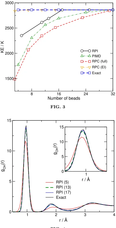
The same trend in convergence of the different PIMD acceleration methods is evident in Fig. 3, which shows results for calculations of the average quantum ki-netic energy of the system, calculated using the virial estimator.70 As in Fig. 2, and as expected, RPC(EI)
8 16 24 32
Number of beads -40
-30 -20 -10
V / kJ mol
-1
RPI PIMD RPC (EI) RPC (full)
Exact
FIG. 2
converges on the corret results usingn= 7 ring-polymer beads for the intermolecular term andn= 32 beads for the intramolecular term, whereas the RPC(full) method again converges more slowly than even the standard PIMD method. In the case of the kinetic energy ex-pectation value, we find that the exact value is obtained when usingn0 ≥17, which is slightly worse than in the case of the potential energy (Fig. 2), but still results in a simulation which requires roughly half the number of PES and force evaluations to obtain the exact results when compared to PIMD. The difference in convergence between Figs. 2 and 3 is most likely due to the fact that potential energy values were used to optimize the value of the GPR width-parameterγ=α, as described above, and then the optimized values for eachn0 were used to calculate all other properties. It seems likely that, if one were to optimise the GPR parameters to simultaneously match both kinetic energy and potential energy for se-lected configurations, the convergence of RPI illustrated in Fig. 3 should improve. Nevertheless, the results of both Figs. 2 and 3 clearly demonstrate that RPI can in-deed converge on exact quantum result using around 50% of the PES and forces evaluations required by standard PIMD.
While calculating individual averaged values, such as quantum potential or kinetic energy, is a good demon-stration that RPI is converging on the correct PIMD properties, a further test is in assessing whether the larger-scale structural properties of the system are cor-rect. Figure 4 shows the O−−H radial distribution func-tion (RDF), gOH(r) calculated using RPI with
9
8 16 24 32
Number of beads
1500 2000 2500 3000
KE / K RPI
PIMD RPC (full) RPC (EI) Exact
FIG. 3
1 2 3 4
r / Å 0
5 10 15
gOH
(r)
RPI (5) RPI (13) RPI (17) Exact
1 r / Å 0
5 10 15
gOH
(r)
FIG. 4
We find that the RDF calculated by RPI is essentially converged using about n0 = 13 GPR reference beads,
with very small error relative to the exact PIMD result. This simulation clearly demonstrates that the atomic-level structure obtained in RPI simulations is the same as that obtained in a full PIMD simulation.
The overall conclusion of the results of Figs. 2-4 is that RPI can clearly converge on exact PIMD simulation re-sults, yet reduces the number of required PES and force evaluations by at least a factor of two relative to con-verged PIMD. Perhaps more importantly, we emphasize that RPI is directly applicable to more complex PESs, including those generated by ab initio electronic struc-ture methods. Compared to evaluation of the PES, the
additional computational overhead required for RPI is very small, and the method itself only requires minor modifications to any standard PIMD code. As a final point, we note that RPI could also be used within the context of other RPC methods, notably the reference-potential based schemes proposed recently,20,51providing a hybrid method which simultaneously accelerates the overall PIMD scheme and the evaluation of the reference potential on the ring-polymer.
IV. CONCLUSIONS
[image:10.612.56.298.50.526.2]In this Article, we have suggested a new approach to accelerating path-integral simulations. Instead of rely-ing on evaluatrely-ing the PES and forces on a contracted ring-polymer, as has been proposed previously, our RPI method instead uses the idea of interpolating the PES values around the ring-polymer, using PES evaluations at just a few selected positions around the ring-polymer. For liquid water at 298 K, described with the q-TIP4P/F empirical water model, we have found that RPI converges on exact PIMD results, but requires just around 50% of the total PES and force evaluations. In contrast to RPC-based methods, RPI is directly applicable to any PES, in-cludingab initiomethods, and requires only small mod-ifications to any existing PIMD code. As noted above, we are now exploring how RPI could be combined with existing RPC methods to further accelerate convergence of properties in PIMD simulations.
ACKNOWLEDGEMENTS
SJB gratefully acknowledges award of a studentship from the EPSRC. Computing facilities were provided by the Scientific Computing Research Technology Platform (SC-RTP) of the University of Warwick. Data from Figs. ??....
1R. P. Feynman and A. R. Hibbs,Quantum mechanics and path
integrals (McGraw-Hill, New York, 1965).
2D. Marx and J. Hutter,Ab initio molecular dynamics: Basic
the-ory and advanced methods(Cambridge University Press, 2009).
3A. M. Reilly, S. Habershon, C. A. Morrison, and D. W. H. Rankin, J. Chem. Phys.132, 094502 (2010).
4A. M. Reilly, S. Habershon, C. A. Morrison, and D. W. H. Rankin, J. Chem. Phys.132, 134511 (2010).
5T. E. Markland and D. E. Manolopoulos, J. Chem. Phys.129, 024105 (2008).
6M. Ceriotti, M. Parrinello, T. E. Markland, and D. E. Manolopoulos, J. Chem. Phys.133, 124104 (2010).
7M. Ceriotti, D. E. Manolopoulos, and M. Parrinello, J. Chem. Phys.134, 084104 (2011).
8M. Parrinello and A. Rahman, J. Chem. Phys.80, 860 (1984). 9R. Ram´ırez, C. P. Herrero, A. Antonelli, and E. R. Hern´andez,
J. Chem. Phys.129, 064110 (2008).
10J. Morales and K. Singer, Mol. Phys.73, 873 (1991).
11R. P. Steele, J. Zwickl, P. Shushkov, and J. C. Tully, J. Chem. Phys.134, 074112 (2011).
13S. Habershon and D. E. Manolopoulos, J. Chem. Phys. 135, 224111 (2011).
14S. Habershon, Phys. Chem. Chem. Phys.16, 9154 (2014). 15T. Spura, C. John, S. Habershon, and T. D. K¨uhne, Mol. Phys.
113, 808 (2015).
16S. Habershon, T. E. Markland, and D. E. Manolopoulos, J. Chem. Phys.131, 024501 (2009).
17A. Wallqvist and B. Berne, Chem. Phys. Lett.117, 214 (1985). 18M. Ceriotti, M. Parrinello, T. E. Markland, and D. E.
Manolopoulos, J. Chem. Phys.133, 124104 (2010).
19V. Kapil, J. VandeVondele, and M. Ceriotti, J. Chem. Phys. 144, 054111 (2016).
20O. Marsalek and T. E. Markland, J. Chem. Phys.144, 054112 (2016).
21R. A. Kuharski and P. J. Rossky, J. Chem. Phys.82, 5164 (1985). 22L. H. de la Pena and P. G. Kusalik, J. Chem. Phys.121, 5992
(2004).
23L. H. de la Pena and P. G. Kusalik, J. Chem. Phys.125, 054512 (2006).
24S. Habershon, G. S. Fanourgakis, and D. E. Manolopoulos, J. Chem. Phys.129, 074501 (2008).
25S. Habershon and D. E. Manolopoulos, J. Chem. Phys. 131, 244518 (2009).
26T. F. M. III and D. E. Manolopoulos, J. Chem. Phys.123, 154504 (2005).
27B. Chen, I. Ivanov, M. L. Klein, and M. Parrinello, Phys. Rev. Lett.91, 215503 (2003).
28C. Alhambra, J. Gao, J. C. Corchado, J. Vill`a, and D. G. Truh-lar, J. Am. Chem. Soc.121, 2253 (1999).
29N. Boekelheide, R. Salom´on-Ferrer, and T. F. Miller III, Proc. Nat. Acad. Sci. USA108, 16159 (2011).
30D. G. Truhlar, J. Gao, C. Alhambra, M. Garcia-Viloca, J. Cor-chado, M. L. S´anchez, and J. Vill`a, Acc. Chem. Res.35, 341 (2002).
31M. H. M. Olsson, P. E. M. Siegbahn, and A. Warshel, J. Am. Chem. Soc.126, 2820 (2004).
32I. R. Craig and D. E. Manolopoulos, J. Chem. Phys.121, 3368 (2004).
33I. R. Craig and D. E. Manolopoulos, J. Chem. Phys.122, 084106 (2005).
34I. R. Craig and D. E. Manolopoulos, J. Chem. Phys.123, 034102 (2005).
35T. F. Miller and D. E. Manolopoulos, J. Chem. Phys.122, 184503 (2005).
36B. J. Braams and D. E. Manolopoulos, J. Chem. Phys. 125, 124105 (2006).
37A. R. Menzeleev and T. F. Miller, J. Chem. Phys.132, 034106 (2010).
38S. Habershon, B. J. Braams, and D. E. Manolopoulos, J. Chem. Phys.127, 174108 (2007).
39T. E. Markland, S. Habershon, and D. E. Manolopoulos, J. Chem. Phys.128, 194506 (2008).
40X. C. Huang, S. Habershon, and J. M. Bowman, Chem. Phys. Letters450, 253 (2008).
41S. Habershon, D. E. Manolopoulos, T. E. Markland, and T. F. Miller, Annu. Rev. Phys. Chem.64, 387 (2013).
42T. J. H. Hele, M. J. Willatt, A. Muolo, and S. C. Althorpe, J Chem Phys142, 191101 (2015).
43E. Geva, Q. Shi, and G. A. Voth, J. Chem. Phys. 115, 9209 (2001).
44G. A. Voth, Adv. Chem. Phys.93, 135 (2007).
45S. Jang and G. A. Voth, J. Chem. Phys.111, 2371 (1999). 46J. Cao and G. A. Voth, J. Chem. Phys.100, 5106 (1994). 47F. Paesani and G. A. Voth, J. Chem. Phys.132, 014105 (2010). 48J. O. Richardson and S. C. Althorpe, J. Chem. Phys.131, 214106
(2009).
49A. R. Menzeleev, N. Ananth, and T. F. Miller, J. Chem. Phys. 135, 074106 (2011).
50T. E. Markland and D. E. Manolopoulos, Chem. Phys. Letters 464, 256 (2008).
51C. John, T. Spura, S. Habershon, and T. D. K¨uhne, Phys. Rev. E93, 043305 (2016).
52T. L. Fletcher and P. L. A. Popelier, J. Chem. Theory Comput. 12, 2742 (2016).
53C. E. Rasmussen and C. Williams,Gaussian Processes for
Ma-chine Learning(MIT Press, 2006).
54S. M. Kandathil, T. L. Fletcher, Y. Yuan, J. Knowles, and P. L. A. Popelier, J. Comput. Chem.34, 1850 (2013).
55M. J. L. Mills and P. L. A. Popelier, Comp. Theo. Chem.975, 42 (2011).
56M. J. L. Mills and P. L. A. Popelier, Theor. Chem. Acc.131, 1 (2012).
57A. P. Bart´ok, M. J. Gillan, F. R. Manby, and G. Cs´anyi, Phys. Rev. B88, 054104 (2013).
58A. P. Bart´ok, M. C. Payne, R. Kondor, and G. Cs´anyi, Phys. Rev. Lett.104, 136403 (2010).
59A. P. Bart´ok and G. Cs´anyi, Int. J. Quantum Chem.115, 1051 (2015).
60D. Chandler,Introduction to Modern Statistical Mechanics (Ox-ford University Press, Ox(Ox-ford, UK, 1987).
61M. E. Tuckerman,Statistical Mechanics: Theory and molecular
simulation (Oxford University Press, 2012).
62T. J. H. Hele and S. C. Althorpe, J. Chem. Phys. 138, 084108 (2013).
63T. J. H. Hele, M. J. Willatt, A. Muolo, and S. C. Althorpe, J. Chem. Phys.142, 134103 (2015).
64G. S. Fanourgakis, T. E. Markland, and D. E. Manolopoulos, J. Chem. Phys.131, 094102 (2009).
65G. Krilov and B. J. Berne, J. Chem. Phys.111, 9147 (1999). 66C. E. Rasmussen and C. K. Williams, Gaussian Processes for
Machine Learning (The MIT Press, Cambridge, Massachusetts,
2006).
67J. P. Alborzpour, D. P. Tew, and S. Habershon, J. Chem. Phys. 145, 174112 (2016).
68L. Mones, N. Bernstein, and G. Cs´anyi, 12, 5110 (2016). 69E. Anderson, Z. Bai, C. Bischof, S. Blackford, J. Demmel, J.
Don-garra, J. Du Croz, A. Greenbaum, S. Hammarling, A. McKenney, and D. Sorensen,LAPACK Users’ Guide, 3rd ed. (Society for In-dustrial and Applied Mathematics, Philadelphia, PA, 1999). 70M. F. Herman, E. J. Bruskin, and B. J. Berne, J. Chem. Phys.