Numerical solution of the first order linear fuzzy differential equations using He$’$s variational iteration method

(1)

https://doi.org/10.26637/MJM0601/0012

Numerical solution of the first order linear fuzzy

differential equations using He

0

s variational iteration

method

M. Ramachandran

1

* and M. Shobanapriya

2

Abstract

In this research, first order linear fuzzy differential equations is considered. This paper compares the He’s variational iteration method (HVIM) and Leapfrog method [17] for solving these equations. He’s variational iteration method is an analytical procedure for finding the solutions of problems which is based on the constructing a variational iterations. The Leapfrog method, based upon Taylor series, transforms the fuzzy differential equation into a matrix equation. The results of applying these methods to the first order linear fuzzy differential equations show the simplicity and efficiency of these methods.

Keywords

Fuzzy differential equations, Fuzzy initial value problems, Leapfrog method, He’s variational iteration method.

AMS Subject Classification

65L80, 65L05.

1_{Department of Mathematics, Government Arts and Science College, Sathyamangalam-638 401, Tamil Nadu, India.} 2_{BT Assistant (Mathematics), Municipal Girls Higher Secondary School, Gobichettipalayam-638 476, Tamil Nadu, India.}

*Corresponding author:1_{[email protected];} 2_{[email protected]}

Article History: Received24September2017; Accepted09December2017 c2017 MJM.

1. Introduction

Knowledge about dynamical systems modelled by differen-tial equations is often incomplete or vague. It concerns, for example, parameter values, functional relationships, or initial conditions. The well-known methods for solving analytically or numerically initial value problems can only be used for finding a selected system behaviour, e.g., by fixing the un-known parameters to some plausible values. However, in this

case, it is not possible to describe the whole set of system behaviours compatible with our partial knowledge.

The topics of fuzzy differential equations, which attracted a growing interest for some time, in particular, in relation to the fuzzy control, have been rapidly developed recent years. The concept of a fuzzy derivative was first introduced by S. L. Chang, L. A. Zadeh [2]. It was followed up by D. Dubois, H. Prade [3], who defined and used the extension principle. Other methods have been discussed by M. L. Puri, D. A. Ralescu [16] and R. Goetschel and W. Voxman [5]. Fuzzy differential equations and initial value problems were regularly treated by O. Kaleva [12,13], S. Seikkala [20]. A numerical method for solving first order linear fuzzy differential equations has been introduced by M. Ma, M. Friedman and A. Kandel [15] via the standard Euler method.

(2)

Maheskumar and K. Kanagarajan [14] and S. Sekar and S. Senthilkumar [18]).

In this article we developed numerical methods for first order linear fuzzy differential equations to get discrete solu-tions via He’s variational iteration method which was studied by Sekar et al. [19]. The subject of this paper is to try to find numerical solutions of first order linear fuzzy differential equations using He’s variational iteration method and com-pare the discrete results with the Leapfrog method which is presented previously by Sekar et al. [17]. Finally, we show the method to achieve the desired accuracy. Details of the structure of the present method are explained in sections. We apply He’s variational iteration method and Leapfrog method for first order linear fuzzy differential equations. In Section 4, it’s proved the efficiency of the He’s variational iteration method. Finally, Section 5 contains some conclusions and directions for future expectations and researches.

2. He’s Variational Iteration Method

In this section, we briefly review the main points of the pow-erful method, known as the He’s variational iteration method [6]-[11]. This method is a modification of a general Lagrange multiplier method proposed by [6]-[11]. In the variational iteration method, the differential equation

L[u(t)] +N[u(t)] =g(t) (2.1)

is considered, whereLandNare linear and nonlinear opera-tors, respectively andg(t)is an inhomogeneous term. Using the method, the correction functional

un+1(t) =un(t) + Z

λ[L[un(s)] +N[u˜n(s)]−g(s)]ds (2.2)

is considered, whereλ is a general Lagrange multiplier,unis

the nth approximate solution and ˜unis a restricted variation

which meansδu˜n=0. In this method, first we determine the

Lagrange multiplierλ that can be identified via variational theory, i.e. the multiplier should be chosen such that the correction functional is stationary, i.e. δu˜n+1(un(t),t) =0.

Then the successive approximationun,n≥0 of the solution uwill be obtained by using any selective initial functionu0

and the calculated Lagrange multiplierλ. Consequentlyu= limn→∞un. It means that, by the correction functional (2.2)

several approximations will be obtained and therefore, the exact solution emerges at the limit of the resulting successive approximations.

3. General format for Fuzzy initial value

problems

Consider a first-order fuzzy initial value differential equation is given by

y0(t) = f(t,y(t)),t∈[t0,T],y(t0) =y0

whereyis a fuzzy function oft,f(t,y)is a fuzzy function of the crisp variablet and the fuzzy variabley,y0 is the fuzzy

derivative ofyandy(t0=y0is a parallelogram or a

parallelo-gram shaped fuzzy number. We denote the fuzzy functiony

byy= [y,y. It means that the r-level set ofy(t)fort∈[t0,T]

is

[y(t)]_r= [y(t;r),y(t;r)],[y(t0)]r= [y(t0;r),y(t0;r)],r∈(0,1]

we writef(t;y) = [f(t;y),f(t;y)]andf(t;y) =F[t,y,y],f(t;y) = G[t,y,y]. Because ofy0(t) =f(t,y)we have

f(t;y(t;r)) =F[t;y(t;r),y(t;r)]

By using the extension principle, we have the membership function

f(t;y(t))(s) =Sup{y(t)(τ)/s= f(t,τ)},s∈R

so fuzzy numberf(t;y(t)). From this it follows that

[f(t;y(t))]r= [f(t,y(t;r)),f(t,y(t;r))],r∈[0; 1]

where

f(t,y(t;r)) =min{f(t,u)/u∈[y(t)]r}

f(t,y(t;r)) =max{f(t,u)/u∈[y(t)]r}

Definition 3.1. A function f :R→RF is said to be fuzzy continuous function, if for an arbitrary fixed t0∈R andε>

0,δ >0such that|t−t0<δ⇒D[f(t),f(t0)]|<εexists.

In this paper we also consider fuzzy functions which are continuous in metricD. Then the continuity of f(t,y(t);r)

guarantees the existence of the definition of f(t,y(t);r)for

t∈[t0,T]andr∈[0,1][M. Ma, M. Friedman and A. Kandel

[15]]. Therefore, the functionsGandFcan be definite too.

4. Numerical Experiments

In this section, the exact solutions and approximated solutions obtained by He’s variational iteration method and Leapfrog method. To show the efficiency of the He’s variational it-eration method, we have considered the following problem taken from C. Duraisamy and B. Usha [4] and T.Jayakumar, D.Maheskumar and K.Kanagarajan [14], with step sizer=

0.1 along with the exact solutions.

(3)

4.1 Example

Consider the initial value problem [C. Duraisamy and B. Usha [4]]

y0(t) =t f(t),t∈[0,1]

with initial conditiony(0) = (1.01+0.1r√e,1.5+0.1r√e)

The exact solution att=0.1 is given by

Y(0.1,r) = [(1.01+0.1r√e)e0.0005,(1.5+0.1r√e)e0.0005],

0≤r≤1

4.2 Example

Consider the fuzzy initial value problem [M. Ma, M. Friedman and A. Kandel [15]]

y0(t) =y(t),t∈I= [0,1]

with initial conditiony(0) = (0.75+0.25r,1.125−0.125r),

0<r≤1

The exact solution is given by

Y1(t,r) =y1(0;r)et,Y2(t,r) =y2(0;r)etwhich att=1

4.3 Example

Consider the fuzzy initial value problem [James J. Buckley and Thomas Feurihg [1]]

y0(t) =c1y2(t) +c2

with initial conditiony(0) =0

whereci>0, fori=1,2 are triangular fuzzy numbers.

The exact solution is given by

Y1(t;r) =l1(r)tan(w1(r)t), Y2(t;r) =l2(r)tan(w2(r)t),

with

l1(r) = p

c2,1(r)/c1,1(r),l2(r) = p

c2,2(r)/c1,2(r) w1(r) =

p

c1,1(r)/c2,1(r),w2(r) = p

c1,2(r)/c2,2(r)

where[c1]r= [c1,1(r),c1,2(r)]and[c2]r= [c2,1(r),c2,2(r)] c1,1(r) =0.5+0.5r,c1,2(r) =1.5−0.5r

c2,1(r) =0.75+0.25r,c2,2(r) =1.25−0.25r

The r-level sets ofy0(t)are

Y₁0(t;r) =c2,1(r)sec2(w1(r)t), Y₂0(t;r) =c2,2(r)sec2(w2(r)t),

which defines a fuzzy number. We have

f1(t,y,r) =min{|c1u2+c2|u∈[y1(t;r),y2(t;r)], c1∈[c1,1(r),c1,2(r)],c2∈[c2,1(r),c2,2(r)]}

f2(t,y,r) =max{|c1u2+c2|u∈[y1(t;r),y2(t;r)], c1∈[c1,1(r),c1,2(r)],c2∈[c2,1(r),c2,2(r)]}

5. Conclusion

He’s variational iteration method is a powerful, accurate, and flexible tool for solving many types of fuzzy differential equa-tions (problems) in scientific computation. The obtained ap-proximate solutions of the first order linear fuzzy differential equations are compared with exact solutions and it reveals that the He’s variational iteration method works well for finding the approximate solutions. From the Tables 1 -– 4, one can observe that for most of the time intervals, the absolute error

Figure 1.Error estimation of Example 4.1 aty1

(4)

Table 1.He’s variational iteration method – Error Calculations

Example 4.1 Example 4.2

r y1 y2 y1 y2

0.1 1.00E-11 1.00E-11 6.00E-11 6.00E-11 0.2 2.00E-11 2.00E-11 7.00E-11 7.00E-11 0.3 3.00E-11 3.00E-11 8.00E-11 8.00E-11 0.4 4.00E-11 4.00E-11 9.00E-11 9.00E-11 0.5 5.00E-11 5.00E-11 1.00E-10 1.00E-10 0.6 6.00E-11 6.00E-11 1.10E-10 1.10E-10 0.7 7.00E-11 7.00E-11 1.20E-10 1.20E-10 0.8 8.00E-11 8.00E-11 1.30E-10 1.30E-10 0.9 9.00E-11 9.00E-11 1.40E-10 1.40E-10 1.0 1.00E-10 1.00E-10 1.50E-10 1.50E-10

Table 2.Leapfrog Method – Error Calculations Example 4.1 Example 4.2

r y1 y2 y1 y2

0.1 1.00E-09 1.00E-09 6.00E-09 6.00E-09 0.2 2.00E-09 2.00E-09 7.00E-09 7.00E-09 0.3 3.00E-09 3.00E-09 8.00E-09 8.00E-09 0.4 4.00E-09 4.00E-09 9.00E-09 9.00E-09 0.5 5.00E-09 5.00E-09 1.00E-08 1.00E-08 0.6 6.00E-09 6.00E-09 1.10E-08 1.10E-08 0.7 7.00E-09 7.00E-09 1.20E-08 1.20E-08 0.8 8.00E-09 8.00E-09 1.30E-08 1.30E-08 0.9 9.00E-09 9.00E-09 1.40E-08 1.40E-08 1.0 1.00E-08 1.00E-08 1.50E-08 1.50E-08

Table 3.He’s variational iteration method – Error Calculations

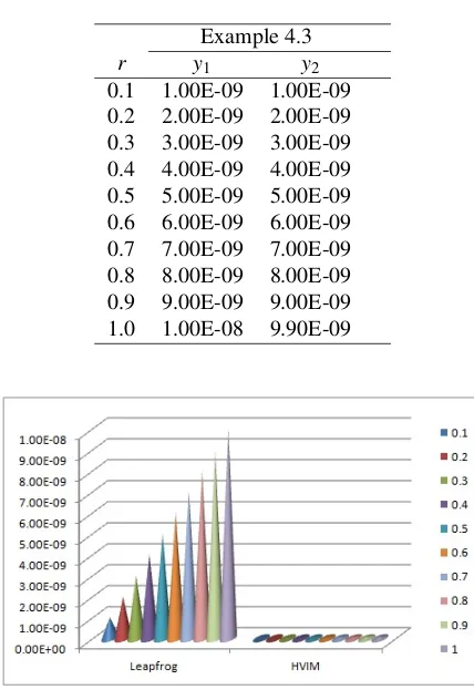
Example 4.3

r y1 y2

0.1 1.00E-11 1.00E-11 0.2 2.00E-11 2.00E-11 0.3 3.00E-11 3.00E-11 0.4 4.00E-11 4.00E-11 0.5 5.00E-11 5.00E-11 0.6 6.00E-11 6.00E-11 0.7 7.00E-11 7.00E-11 0.8 8.00E-11 8.00E-11 0.9 9.00E-11 9.00E-11 1.0 1.00E-10 9.90E-11

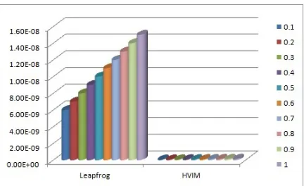
is less in He’s variational iteration method when compared to the Leapfrog method [18], which yields a little error, along with the exact solutions. From the Figures 1 -– 6, it can be predicted that the error is very less in He’s variational iteration method when compared to the Leapfrog method. Hence, He’s

Table 4.Leapfrog Method – Error Calculations Example 4.3

r y1 y2

0.1 1.00E-09 1.00E-09 0.2 2.00E-09 2.00E-09 0.3 3.00E-09 3.00E-09 0.4 4.00E-09 4.00E-09 0.5 5.00E-09 5.00E-09 0.6 6.00E-09 6.00E-09 0.7 7.00E-09 7.00E-09 0.8 8.00E-09 8.00E-09 0.9 9.00E-09 9.00E-09 1.0 1.00E-08 9.90E-09

variational iteration method is more suitable for studying first order linear fuzzy differential equations.

References

[1] _{J. J. Buckley and T. Feurihg, Introduction to Fuzzy Partial}

Differential Equations,Fuzzy Sets and Systems, 110(1) (2000), 43-54.

[2] _{S. L. Chang and L. A. Zadeh, On fuzzy mapping and}

control,IEEE Transactions on Systems, Man, and Cyber-netics, 2 (1972), 30-34.

[3] _{D. Dubois and H. Prade, Towards fuzzy differential}

cal-culus.III. Differentiation,Fuzzy Sets and Systems, 8(3) (1982), 225-233.

[4] _{C. Duraisamy and B. Usha, Another Approach to}

Solu-tion of Fuzzy Differential EquaSolu-tions,Applied Mathemati-cal Sciences, 4(16) (2010), 777-790.

[5] _{R. Goetschel and W. Voxman, Elementary calculus,}_Fuzzy Sets and Systems, 18 (1986), 31-43.

[6] _{J. H. He, A new approach to nonlinear partial differential}

equations,Commun Nonlinear Sci Numer Simulat, 2(4) (1997), 203-205.

[7] _{J. H. He, Approximate analytical solution for seepage}

(5)

[8] _{J. H. He, Variational iteration method – a kind of}

non-linear analytical technique: some examples,Int. J. Non-linear Mech., 34(1999), 699-708.

[9] _{J. H. He, Variational iteration method for autonomous}

or-dinary differential systems,Appl. Math. Comput., 114(2– 3) (20000, 115-123.

[10] _{J. H. He, Variational iteration method – Some recent}

results and new interpretations,J. Comput. Appl. Math., 207 (2007), 3–17.

[11] _{J. H. He, Variational principle for some nonlinear partial}

differential equations with variable coefficients,Chaos Solitons Fractals, 19 (2004), 847–851.

[12] _{O. Kaleva, Fuzzy differential equations,}_{Fuzzy Sets and} Systems, 24(3) (1987), 301-317.

[13] _{O. Kaleva, “The Cauchy problem for fuzzy differential}

equations,” Fuzzy Sets and Systems, vol. 35, no. 3, pp. 389—396, 1990.

[14] _{T. Jayakumar, D. Maheskumar and K. Kanagarajan,}

Nu-merical Solution of Fuzzy Differential Equations by Runge Kutta Method of Order Five,Applied Mathemati-cal Sciences, 6(60) (2012), 2989-3002.

[15] _{M. Ma, M. Friedman and A. kandel, Numerical Solutions}

of Fuzzy Differential Equations,Fuzzy Sets and Systems, 105 (1999), 133-138.

[16] _{M. L. Puri and D. A. Ralescu, Differentials of fuzzy}

func-tions,Journal of Mathematical Analysis and Applications, 91(2) (1983), 552-558.

[17] _{S. Sekar and K. Prabhavathi, Numerical solution of first}

order linear fuzzy differential equations using Leapfrog method,IOSR Journal of Mathematics, 10(5) (2014), 07-12.

[18] _{S. Sekar and S. Senthilkumar, Single Term Haar Wavelet}

Series for Fuzzy Differential Equations, International Journal of Mathematics Trends and Technology, 4(9) (2013), 181-188.

[19] _{S. Sekar and B. Venkatachalam alias Ravikumar,}

Nu-merical Solution of linear first order Singular Systems Using He’s Variational Iteration Method,IOSR Journal of Mathematics, 11(5) (2015), 32-36.

[20] _{S. Seikkala, On the fuzzy initial value problem,}_Fuzzy Sets and Systems, 24(3) (1987), 319-330.

? ? ? ? ? ? ? ? ?

ISSN(P):2319−3786 Malaya Journal of Matematik

ISSN(O):2321−5666

Numerical solution of the first order linear fuzzy differential equations using He$’$s variational iteration method