Reliability Measure of an Integrated H/W and S/W System with Redundancy and Preventive maintenance

(1)

Reliability Measure of an Integrated H/W and S/W System with

Redundancy and Preventive maintenance

Ashish Kumar

∗

Department of Mathematics, Manipal University Jaipur, Jaipur-303007, Rajasthan, India.

Abstract

The purpose of the study is to evaluate the reliability measures of an integrated h/w and s/w system with the concepts of redundancy and preventive maintenance. A stochastic model is developed considering two-identical units of the system- one unit is initially operative and other is in cold standby. In each unit h/w and s/w work together and may fail independently from normal mode. There is a single server who visits the system immediately to h/w repair and s/w up-gradation. The preventive maintenance of the system (unit) is conducted by the server after a maximum operation time. The failure time of h/w and s/w follows negative exponential distribution while the distributions of preventive maintenance, h/w repair and s/w up-gradation times are taken as arbitrary. The semi-Markov process and regenerative point technique is adopted to derive expressions for various measures of system effectiveness. The behaviour of some important reliability measures has been observed graphically giving particular values to various costs and parameters.

Keywords:Integrated h/w and s/w System, Redundancy, H/w Repair, S/w Up-gradation, Preventive Maintenance, Maximum Operation

Time and Reliability Measures.

1

Introduction

Now a day’s integrated h/w and s/w systems are of growing importance because of their use in almost all academic, business and industrial sectors. The continued operation and ageing of these systems gradually reduce their performance, reliability and safety. Therefore, a major challenge to the engineers and researchers is to develop such systems which can produce failure free services to the users with least cost. The method of redundancy has been used in many industrial systems not only to attain better reliability but also to reduce the

frequency of failure up to a desired extent. Goel and Sharma[1]and Singh[2]discussed stochastically the two

unit standby system under different repair policies of the server. But the technique of redundancy has not been

used much more in case of integrated h/w and s/w systems. A few researchers including Malik and Anand[3]

obtained reliability measures for a computer system by taking a redundant unit in cold standby. Further, it is proved that preventive maintenance can slow the deterioration process of operating system and restore them in a younger age or state. Thus, the method of preventive maintenance can be used to improve the

performance of these systems. Recently, Malik and Kumar[4] investigated a reliability model for a computer

system conducting preventive maintenance after a maximum operation time.

To strengthen the existing literature, here reliability measures for an integrated h/w and s/w system are obtained by introducing the concepts of redundancy and preventive maintenance. A stochastic model is developed considering two-identical units of the system- one unit is initially operative and other is in cold standby. In each unit h/w and s/w work together and may fail independently from normal mode. There

∗_{Corresponding author.}

(2)

is a single server who visits the system immediately to h/w repair and s/w up-gradation. The preventive maintenance of the system (unit) is conducted by the server after a maximum operation time. The failure time of h/w and s/w follows negative exponential distribution while the distributions of preventive maintenance, h/w repair and s/w up-gradation times are taken as arbitrary. The semi-Markov process and regenerative point technique is adopted to derive expressions for various measures of system effectiveness such as mean time to system failure, availability, busy period of the server due to preventive maintenance, busy period of the server due to h/w repair, busy period of the server due to software up-gradation, expected number of software up-gradations and expected number of visits of the server. The behaviour of some important reliability measures has been observed graphically giving particular values to various costs and parameters.

Notations

N0 : The unit is operative and in normal mode

Cs : The unit is cold standby

a/b : Probability that the system has hardware/software failure

λ1/λ2 : Constant failure rate of hardware/software

α0 : Constant rate of Maximum Operation Time

Pm/PM : The unit is under preventive Maintenance/under preventive maintenance

continuously from previous state

WPm/WPM : The unit is waiting for preventive Maintenance/waiting for preventive

maintenance continuously from previous state

HFur/HFUR : The hardware is failed and is under repair/under repair continuously from

previous state

HFwr/HFWR : The hardware is failed and is waiting for repair/waiting for repair continuously

from previous state

SFurp/SFURP : The software is failed and is under up-gradation/under up-gradation

continuously from previous state

SFwrp/SFWRP : The software is failed and is waiting for up-gradation/waiting for up-gradation continuously from previous state

h(t)/H(t) : pdf/cdf of software up-gradation time

g(t)/G(t) : pdf/cdf of repair time of the hardware

f(t)/F(t) : pdf/cdf of the time for preventive maintenance of the unit

qij_(t)_/_Qij_(t) _: _{pdf/cdf of passage time from regenerative state}_i_{to a regenerative state} _j_{or to a}

failed statejwithout visiting any other regenerative state in(0,t]

pd f/cd f : Probability density function/ Cumulative density function

qij·kr(t)/Qij·kr(t) : pdf/cdf of direct transition time from regenerative stateito a regenerative statej

or to a failed statejvisiting statek,ronce in(0,t]

µi(t) : Probability that the system up initially in state Si ∈ E is up at time t without

visiting to any regenerative state

Wi(t) : Probability that the server is busy in the stateSiup to time ‘t’ without making any

transition to any other regenerative state or returning to the same state via one or more non-regenerative states.

mij : Contribution to mean sojourn time(µi)in stateSiwhen system transit directly to

stateSjso thatµi=∑

j

mijandmij= R

tdQij(t) =−q∗

0

ij(0)?

(3)

Transition Probabilities and Mean Sojourn Times

Simple probabilistic considerations yield the following expressions for the non-zero elements

pij=Qij(∞) = Z

qij(t)dt (1.1)

as

p01= R

0α

A , p

02 ₌

R

1aλ

A ,

p03= R

2bλ

A , p

10 ₌ _f∗_(A)_,

p1.10₌

R

1aλ

A [1−f

∗_{(A)] =} _p12.10_, _p1.12₌

R

2bλ

A [1−f

∗_{(A)] =} _p13.12_,

p1.4= R

0α

A [1−f

∗_{(A)] =} _p11.4_, _p20 ₌_g∗₍_A)_,

p29= R

0α

A [1−g

∗_{(A)] =} _p21.9_, _p27 ₌

R

2bλ

A [1−g

∗_{(A)] =} _p23.7_,

p28₌

R

1aλ

A [1−g

∗_{(A)] =} _p22.8_, _p30 ₌_h∗_(A)_,

p35= R

1aλ

A [1−h

∗_{(A)] =} _p32.5_, _p3.11₌

R

0α

A [1−h

∗_{(A)] =} _p3,1.11_,

p41= f∗(s), p36 =

R

2bλ

A [1−h

∗_{(A)] =} _p33.6_,

p52₌_h∗_(s)_, _p63 ₌_h∗_(s)_,

p73=g∗(s) =p82= p91, p10.2= f∗(s),

p11.1=h∗(s), p12.3= f∗(s)

                                                                                                 (1.2)

whereA=R

1aλ+

R

2bλ+

R

0α.

It can be easily verified that

p01₊_p02₊_p03 ₌ _p10₊_p14₊_p1.10₊_p1.12₌ _p20₊_p27₊_p29₊_p28

= p30+p35+p3.11+p36 =p41= p52 =p63= p73 = p82 =p91= p10.2=p11.1=p12.3

= p10₊_p12.10₊_p11.4₊_p13.12₌_p20₊_p21.9₊_p22,8₊_p23.7

= p30+p31.11+p32.5+p33.6=1

                             (1.3)

The mean sojourn times(µi)is the stateSiareµ

µ0= R 1

1aλ+

R

2bλ+

R

0α

, µ1= R 1

1aλ+

R

2bλ+

R

0α+α

,

µ2= R 1

1aλ+

R

2bλ+

R

0α+θ

, µ3= R 1

1aλ+

R

2bλ+

R

0α+

R β,

µ0₁= 1

α, µ 0 2= 1 θ, µ 0 3= 1 β                  (1.4)

The statesS0, S1,S2 and S3 are regenerative states whileS4, S5, S6, S7, S8,S9, S10, S11 and S12, are

non-regenerative states. ThusE = {S0,S1,S2,S3}. The possible transition between states along with transition

(4)

: Operative State : Failed State  : Regenerative Point S2

S3

S1

S0 N_Cs0

N0

Pm

SFurp N0

N0

HFur

0

f(t) g(t)

h(t) b2 a1

S5 S7

b2

S12

S11

S6

f(t) b2

SFURP SFwrp

SFURP Wpm

h(t)

0

h(t)

HFUR SFwrp

b2

PM SFwrp SFURP

HFwr _h(t)

a1 S8

g(t) a1

HFUR HFwr

f(t)

S10PM

HFwr

a1

S4

WPm PM _f(t)

0

S9

0

HFUR WPm

g(t)

Figure 1:

Reliability and Mean Time to System Failure (MTSF)

Let φi(t)be the cdf of first passage time from the regenerative state ito a failed state. Regarding the failed

state as absorbing state, we have the following recursive relations forφi(t):

ϕi(t) =

∑

j

Qi,j(t) +rϕj(t) +

∑

k

Qi,j(t), (1.5)

where jis an un-failed regenerative state to which the given regenerative stateican transit andkis a failed

state to which the stateican transit directly. Taking LST of above relation (1.5) and solving for ˜φ0(s). We have

R∗(s) =1−φ˜0(s)

s (1.6)

The reliability of the system model can be obtained by taking Laplace inverse transform of (1.6). The mean time to system failure (MTSF) is given by

MTSF=lim

s→0

1−φe0(s)

s =

N1

D1

(1.7)

whereN1₌_µ

0+p01µ1+p02µ2+ +p03µ3andD1=1−p01p10−p02p20−p03p30.

2 Steady State Availability

Let Ai(t) be the probability that the system is in up-state at instant ‘t’ given that the system entered

regenerative stateiatt=0. The recursive relations forAi(t)are given as

Ai(t) =Mi(t) +

∑

j

a(_ijn)(t)cAj(t) (2.8)

wherejis any successive regenerative state to which the regenerative stateican transit throughntransitions.

(5)

regenerative state, we have is

M0(t) =e−(aλ1+bλ2+α0) t

, ,M1(t) =e−(aλ1+bλ2+α0) t

F(t), M2(t) =e−(aλ1+bλ2+α0)

t

G(t), ,M3(t) =e−(aλ1+bλ2+α0) t

H(t), (2.9)

Taking LT of above relations (2.8) and solving forA∗₀(s). The steady state availability is given by

A0(∞) =lim

s→0sA

∗ 0(s) =

N2

D2

, (2.10)

where

N2=µ0[(1−p11.4){(1−p22.8)(1−p33.6)−p23.7p32.5} −p12.10{(1−p33.6)p21.9+p31.11p23.7} −p13.12{p21.9p32.5+ (1−p22.8)p33.6}] +µ1[p01{(1−p22.8)(1−p33.6)−p23.7p32.5}

+p02{(1−p33.6)p21.9+p31.11p23.7}+p03{p21.9p32.5+ (1−p22.8)p33.6}]

+µ2[p01{p12.10(1−p33.6) +p13.12p32.5}+p02{(1−p33.6)(1−p11.4)−p31.11p13.12}

+p03{p31.11p12.10+ (1−p11.4)p32.5}] +µ3[p01{p12.10p23.7+p13.12(1−p22.8)}

+p02{(1−p11.4)p23.7+p21.9p13.12}+p03{(1−p22.8)(1−p11.14)−p21.9p12.10}]

and

D2=µ0[(1−p11.4){(1−p22.8)(1−p33.6)−p23.7p32.5} −p12.10{(1−p33.6)p21.9+p31.11p23.7} −p13.12{p21.9p32.5+ (1−p22.8)p33.6}] + [p01{(1−p22.8)(1−p33.6)−p23.7p32.5}

+p02{(1−p33.6)p21.9+p31.11p23.7}+p03{p21.9p32.5+ (1−p22.8)p33.6}]

+ [p01{p12.10(1−p33.6) +p13.12p32.5}+p02{(1−p33.6)(1−p11.4)−p31.11p13.12}

+p03{p31.11p12.10+ (1−p11.4)p32.5}] + [p01{p12.10p23.7+p13.12(1−p22.8)}

+p02{(1−p11.4)p23.7+p21.9p13.12}+p03{(1−p22.8)(1−p11.14)−p21.9p12.10}]

Busy Period Analysis for Server

Let BP_i(t), B_iR(t) and BS_i(t) be the probability that the server is busy in preventive maintenance, hardware

repair and software up-gradation of the system (unit) at an instant ‘t’ given that the system entered stateiat

t=0. The recursive relations forB_iP(t),BR_i (t)andB_iS(t)are as follows:

BP_i(t) =Wi(t) +

∑

j

q(_ijn)(t)cBp_J(t) (2.11)

B_iR(t) =Wi(t) +

∑

j

q(_ijn)(t)cBR_J(t) (2.12)

BS_i(t) =Wi(t) +

∑

j

q(_ijn)(t)cBS_J(t) (2.13)

Wherejis any successive regenerative state to which the regenerative stateican transit throughntransitions.

Wi(t)be the probability that the server is busy in stateSidue to PM, h/w repair and s/w up-gradation of the

system up to timetwithout making any transition to any other regenerative state or returning to the same

via one or more non-regenerative states. Taking LT of above relations (2.11) to (2.13) and solving forB∗₀P(s),

B₀∗R(s)and B∗₀S(s). The time for which server is busy due to preventive maintenance, h/w repair and s/w

up-gradation respectively is given by

B₀p=lim s→0sB

∗P

0 (s) =

N₃p D2

, B₀R=lim s→0sB

∗R

0 (s) =

N₃R D2

andBS₀ =lim

s→0sB ∗S

0 (s) =

N₃S D2

(6)

where

N3P=W1∗(0)[p01{(1−p22.8)(1−p33.6)−p23.7p32.5}+p02{(1−p33.6)p21.9+p31.11p23.7}

+p03{p21.9p32.5+ (1−p22.8)p33.6}] (2.14)

N₃P=W₂∗(0)[p01{p12.10(1−p33.6) +p13.12p32.5}+p02{(1−p33.6)(1−p11.4)−p31.11p13.12}

+p03{p31.11p12.10+ (1−p11.4)p32.5}] (2.15)

N₃S =W₂∗(0)[p01{p12.10p23.7+p13.12(1−p22.8)}+p02{(1−p11.4)p23.7+p21.9p13.12}

+p03{(1−p22.8)(1−p11.14)−p21.9p12.10}] (2.16)

Expected Number of S/w Up-gradations

Let RS_i(t) be the expected number of software up-gradations by the server in (0,t] given that the system

entered the regenerative stateiatt=0. The recursive relations forRS_i(t)are given as

RS_i(t) =

∑

j

Q(_i_,n_j)(t)r[δ_j+RS_j(t)]. (2.17)

Where j is any regenerative state to which the given regenerative state i transits and δj = 1, if j is the

regenerative state where the server does job afresh, otherwiseδj=0.

Taking LST of relations (2.17) and solving for ˜RS₀(s). The expected numbers of s/w up-gradations per unit

time are given by

RS₀(∞) =lim s→0R˜

S

0 =

N₄S D2

. (2.18)

WhereD2is already mentioned.

N₄S = [p01{p12.10p23.7+p13.12(1−p22.8)}+p02{(1−p11.4)p23.7+p21.9p13.12}

+p03{(1−p22.8)(1−p11.14)−p21.9p12.10}]

Expected Number of Visits by the Server

LetNi(t)be the expected number of visits by the server in(0,t]given that the system entered the regenerative

stateiatt=0. The recursive relations forNi(t)are given as

Ni(t) =

∑

j

Q(_i_,n_j)(t)r[δ_j+Nj(t)] (2.19)

Where j is any regenerative state to which the given regenerative state i transits and δj = 1, if j is the

regenerative state where the server does job afresh, otherwiseδj=0. Taking LST of relation (2.19) and solving

for ˜N0(s). The expected number of visit per unit time by the ˜N0(s)server are given by

N0(∞) =lim

s→0sN˜0(s) =

N2

D2

, (2.20)

where

N5= [(1−p11.4){(1−p22.8)(1−p33.6)−p23.7p32.5} −p12.10{(1−p33.6)p21.9+p31.11p23.7} −p13.12{p21.9p32.5+ (1−p22.8)p33.6}]

Profit Analysis

The profit incurred to the system model in steady state can be obtained as

(7)

K0=Revenue per unit up-time of the system

K1=Cost per unit time for which server is busy due preventive maintenance

K2=Cost per unit time for which server is busy due to hardware failure

K3=Cost per unit time for which server is busy due to software up-gradation

K4=Cost per unit time s/w up-gradation

K5=Cost per unit time visit by the server

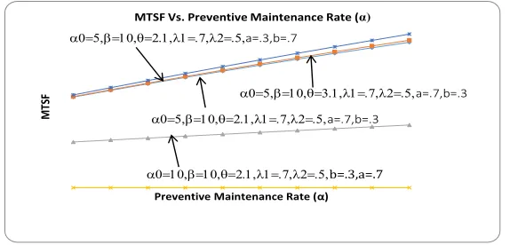
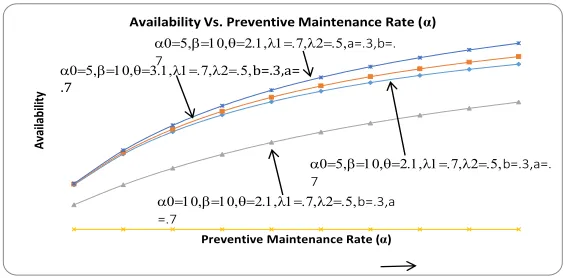
3 Conclusion

By considering a particular caseg(t) = θe−θt_,_{h(t) =} _βe−βt_and _f_{(t) =} _αe−αt_{, the numerical results some}

reliability measures are obtained for the system under study. The graphs for mean time to system failure

(MTSF), availability and profit are drawn with respect to preventive maintenance(α)rate for fixed values

of parameters as shown respectively in Figures 4,??and??. It is revealed that MTSF, Availability and profit

increase with the increase of PM rate(α)and h/w repair rate(θ). But the value of these measures decrease

with the increase of maximum operation time(α0). Thus finally it is concluded that a system in which chances

of h/w failure are high can be made reliable and economical to use (i) By taking one more unit in cold standby.

(ii) By conducting PM of the system after a specific period of time.

(iii) By increasing h/w repair rate in case preventive maintenance of the system is not conducted after a maximum operation time.

Fig. 2: MTSF Vs. Preventive Maintenance Rate (α)

M

TS

F

Preventive Maintenance Rate (α) MTSF Vs. Preventive Maintenance Rate (α)

a0=5,b=10,q=2.1,l1=.7,l2=.5,a=.3,b=.7

a0=10,b=10,q=2.1,l1=.7,l2=.5,b=.3,a=.7

a0=5,b=10,q=3.1,l1=.7,l2=.5,a=.7,b=.3

a0=5,b=10,q=2.1,l1=.7,l2=.5,a=.7,b=.3

(8)

Fig. 3: Availability Vs. Preventive Maintenance Rate (α)

A

vai

lab

ili

ty

Preventive Maintenance Rate (α)

Availability Vs. Preventive Maintenance Rate (α)

a0=5,b=10,q=3.1,l1=.7,l2=.5,b=.3,a= .7

a0=5,b=10,q=2.1,l1=.7,l2=.5,a=.3,b=. 7

a0=5,b=10,q=2.1,l1=.7,l2=.5,b=.3,a=. 7

a0=10,b=10,q=2.1,l1=.7,l2=.5,b=.3,a =.7

Figure 3:

Fig. 4: Profit Vs. Preventive Maintenance Rate (α)

Pr

ofi

t

Preventive Maintenance Rate(α)

Profit Vs. Preventive Maintenance Rate (α)

a0=5,b=10,q=3.1,l1=.7,l2=.5,a=.7,b=.3

a0=5,b=10,q=2.1,l1=.7,l2=.5,a=.3,b=.7

a0=5,b=10,q=2.1,l1=.7,l2=.5,b=.3,a=.7 a0=10,b=10,q=2.1,l1=.7,l2=.5,b=.3,a=.7

K0=5000,K1=150,K2 =350,K3=50,K4=500, K5=100

Figure 4:

References

[1] L.R. Goel and S.C. Sharma, Stochastic analysis of a two-unit standby system with two failure modes and

slow switch,Microelectronics and Reliability, 1989, Vol. 29 (4), pp. 493-498.

[2] S.K. Singh and R.P. Singh, Profit evaluation of a two-unit cold standby system with a provision of rest, Microelectronics and Reliability, 1989, Vol. 29 (5), pp. 705-709.

[3] S.C. Malik and Jyoti Anand, Reliability and economic analysis of a computer system with independent

hardware and software failures,Bulletin of Pure and Applied Sciences, 2010, Vol. 29 E (Math. & Stat.), No. 1,

pp. 141-153.

[4] S.C. Malik and A. Kumar, Reliability modeling of a computer system with priority to s/w replacement

over h/w replacement subject to MOT and MRT,International Journal of Pure and Applied Mathematics,

(9)

Received: November 12, 2015;Accepted: March 25, 2016

UNIVERSITY PRESS