Construction of Co-occurrence Matrix using
Gabor Wavelets for Classification of Arecanuts
by Decision Trees
Suresha M
Kuvempu University Karnataka
India
Ajit Danti
J.N.N College of Engineering Karnataka
India
ABSTRACT
In this paper, a novel method developed for classification of arecanuts based on texture features. A Gabor response co-occurrence matrix (GRCM) is constructed analogous to Gray Level co-occurrence matrix (GLCM). Classification is done using kNN and Decision Tree (DT) classifier based on GRCM features. There are twelve Gabor filters are designed (Four orientations and three scaling) to capture variations in lighting conditions. Results are compared with kNN classifier and found better results. Splitting rules for growing decision tree that are included are ginidiversity index(gdi), twoing rule, and entropy. Proposed approach is experimented on large data set using cross validation and found good success rate in decision tree classifier.
General Terms
Image Processing, Pattern Recognition, Classification.
Keywords
Arecanut, classification, Decision Trees, Gabor response co-occurrence matrix, Gabor Wavelets, Gray level co-co-occurrence matrix, Texture Features.
1.
INTRODUCTION
Arecanut palm (Areca catechu L.,) family Palmae is the source of arecanut referred to as betelnut or supari in India. It is used in Indian and other South countries as a masticatory. It forms one of the ingredients of betel quid commonly in India. It has an integral part in several religious and social ceremonies. Arecanut is largely cultivated in the plains and foot hills of Western Ghats and Eastern regions of India. Area and production in different states indicate that Kerala and Assam account for over 90 percent. Arecanut is grown in Bangladesh, China, Malaysia, Indonesia, Vietnam and Thailand. India accounts for about 57 percent of world production. In the classification of arecanut, color and texture are the most important parameters that allows for the evaluation of their degree of quality, and existence of faults. Also, color along with its level of homogeneity influences the degree of acceptance of consumers, as well as the pricing.
There are six types of arecanuts considered for this work, namely Api, Red Bette (RB), Black Bette (BB), Minne, Gotu and Chaali. In the proposed method, arecanuts are classified using Gabor response co-occurrence matrix (GRCM) features like Contrast, Correlation, Energy and Homogeneity. An experiment is conducted using kNN classifier and Decision tree classifier and the results are discussed. Survey has been
conducted and collected samples from about 15 agricultural fields and eight tender markets.
In the rest of this paper, described some related works briefly in Section 2. The problem is defined in Section 3. Proposed methodology is presented in Section 4, which includes segmentation using watershed segmentation, feature extraction and classification of arecanuts using kNN classifier and decision tree. Experimental results and analysis have been included in Section 5. Finally, conclusions are drawn in Section 6.
2.
LITERATURE REVIEW
Geurts [6]. The two most widely used implementations for decision trees are Leo Breiman [7] and Ross Quinlan C4.5 [8]. What is needed instead is, assuming a binary label space for simplicity, a total ordering of test instances from most likely positive to most likely negative. In this way, a ranking of test instances is obtained. The rank position of an instance depends on the score it receives. Obviously, the mapping from an instance to the probability of belonging to the positive class is a perfect scoring function, but so is any monotone transformation thereof. It follows that a good probability estimator is a good ranker, but not necessarily the other way around. Even more interestingly, improving accuracy does not necessarily decrease the number of ranking errors, and vice versa Peter Flach et al. [9]. The standard performance metric for the supervised ranking setting is the area under the ROC curve, or AUC for short Andrew Bradley [10]. A decision tree, trained in the usual way as a classifier, can be used for ranking by scoring an instance in terms of the frequency of positive examples found in the leaf to which it is assigned. A few papers provide experiments showing that unpruned trees lead to better rankings than standard pruned trees Foster Provost et al. [11], Cesar Ferri et al. [12]. This is counterintuitive at least sight since it is well known, at least for classification accuracy, that pruning prevents or alleviates the over fitting effect and strongly reduces variance. Several other enhancements to the trees have been proposed to improve their ranking performance. Fuzzy decision trees are more advanced in the sense that they model uncertainty around the split values of the features, resulting in soft instead of hard splits. Moreover, they naturally produce scores in the form of membership degrees. Several papers have compared decision trees with their fuzzy variants, but always in terms of classification accuracy Cristina Olaru et al. [13] and references therein. Yet, even though some gains have occasionally been reported, it is still unclear whether fuzzy decision trees can systematically and significantly outperform non-fuzzy trees in terms of classification accuracy. A method proposed the use of multi-way splits for continuous attributes in order to reduce the tree complexity without decreasing classification accuracy. This can be done by intertwining a hierarchical clustering algorithm with the usual greedy decision tree learning Fernando Berzal et al. [14]. A survey on evolutionary algorithms is conducted for decision-tree induction. In this context, most of the paper focuses on approaches that evolve decision trees as an alternate heuristics to the traditional top-down divide-and-conquer approach Barros et al. [15]. Proposed the fuzzy decision tree (FDT)-support vector machine (SVMs) classifier, the node discriminations are implemented using binary SVMs. The tree structure is determined using a class grouping algorithm, which forms the groups of classes to be separated at each internal node, based on the degree of fuzzy confusion between the classes. Effective feature selection is incorporated within the tree building process. FDT-SVM exhibits a number of attractive merits such as enhanced classification accuracy, interpretable hierarchy, and low model complexity. Furthermore, it provides hierarchical image segmentation and has reasonably low computational and data storage demands Moustakidis et al. [16]. Juan Sun et al., [17] Analyzed the effect of different types of noises, compares the tolerance capability of noise between fuzzy decision trees and crisp decision trees, discussed the modified degree of pruning methods in fuzzy and crisp decision trees, addressed the adjustable capability on noise by using different fuzzy reasoning operators in the fuzzy decision tree. Finally the experimental results shows fuzzy decision tree is more
efficient than the crisp decision tree and the post-pruning crisp decision tree. Setiono R et al., [18] presented a novel algorithm for generating oblique decision trees that capitalizes on the strength of both neural networks and decision tree. Oblique decision trees classify the patterns by testing on linear combinations of the input attributes. An oblique decision tree is usually much smaller than the univariate tree generated for the same domain. Algorithm consists of two components: connectionist and symbolic. A three-layer feed forward neural network is constructed and pruned, a decision tree is then built from the hidden unit activation values of the pruned network. An oblique decision tree is obtained by expressing the activation values using the original input attributes. Haiwei Xu et al., [19] proposed an improved random decision trees algorithm by adding tree balance factor for land cover remote sensing classification. Comparison study was conducted to compare the improved random decision trees algorithm with maximum likelihood classification method. The results indicate that the classification accuracy is improved from 81.46% to 87.53% and Kappa coefficient gives up to 0.8524. Pedrycz W et al., [20] proposed a decision trees based on information granules - multivariable entities characterized by high homogeneity or low variability. Granules are developed using fuzzy clustering and play a major role in the growth of the decision trees, they are referred as C-fuzzy decision trees. This form of decision trees involves all variables that are considered for splitting of each node of the tree. A series of experiments is carried out using synthetic and machine learning data sets. Crockett K et al., [21] presented a novel approach to combining multiple decision trees, which combines the power of fuzzy inference techniques and a back-propagation feed forward neural network (BP-FFNN) to improve the classification rate.
3.
PROBLEM DEFINITION
There are many grades of arecanut is available in the market. Qualitative sorting is usually performed by trained inspectors. This type of evaluation is rather expensive and is determined by operators' inconsistency and subjectivity. Machine vision technology offers objective solutions for all these problems and it is considered to be a promise for replacing the traditional human inspection methods in the field of arecanut marketing.
4.
PROPOSED METHODOLOGY
In the proposed method, arecanuts are segmented from the given image. In feature extraction stage Gabor response are obtained using 12 filters. GRCM is constructed and features of GRCM like Contrast, Correlation, Energy and Homogeneity are used for classification of unknown samples using kNN classifier and Decision tree classifier.
4.1
Segmentation
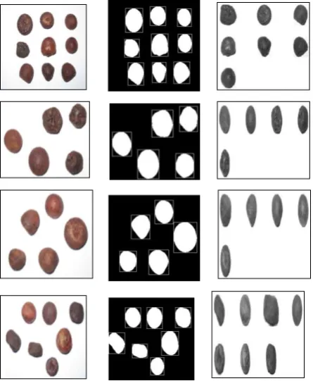
image intensity. Meanwhile, Watershed segmentation also embodies other principal image segmentation methods including discontinuity detection, thresholding and region processing. Because of these factors, watershed segmentation displays more effectiveness and stableness than other segmentation algorithms Rafael C. Gonzalez et al. [22]. Watershed segmentation is an effective method for gray level arecanut image segmentation. To apply watershed segmentation to binary images, there is a need to preprocess the arecanut binary images with distance transform to convert it to gray level images which are suitable for watershed segmentation. The common Distance Transforms (DTs) include Euclidean, City block and Chessboard. Different DTs produce very different watershed segmentation results for the arecanut binary images. For arecanut images containing components of different shapes, it is found that the Chessboard DT can achieve better watershed segmentation results. Each image contains multiple intra class arecanut objects. The segmented image is labeled and each arecanut is extracted from the image as shown in Figure. 1(b) and 1(c) respectively.
(a) Original Image (b) Labeled Image (c) Segmented
Image
Figure 1: Sample Experimental Results
4.2
Feature Extraction
In the feature extraction process, obtained Gabor responses of sample data using Gabor wavelets. With this data determined GRCM features such as Contrast, Correlation, Energy and Homogeneity based on Gabor response of pixels.
4.2.1
Gabor Filter Response
Texture analysis using filters based on Gabor functions falls into the category of frequency-based approaches. These approaches are based on the premise that texture is an image pattern containing a repetitive structure that can be effectively characterized in a frequency domain, such as the Fourier domain. One of the challenges, however, of such an approach
is dealing with the tradeoff between the joint uncertainty in the space and frequency domains. Meaningful frequency based analysis cannot be localized without bound. An attractive mathematical property of Gabor functions is that they minimize the joint uncertainty in space and frequency. They achieve the optimal tradeoff between localizing the analysis in the spatial and frequency domains Newsam et al., [23].The Gabor filter is a linear filter whose impulse response is defined by a harmonic function multiplied by a Gaussian function. Because of the multiplication-convolution property (Convolution theorem), the Fourier transform of a Gabor filter's impulse response is the convolution of the Fourier transform of the harmonic function and the Fourier transform of the Gaussian function and it is given by.
cos
2
'
2
'
'
exp
)
,
,
,
,
;
,
(
22 2 2
x
y
x
y
x
g
(1)
Where x' = xcosθ + ysinθ and y' = xsinθ + ycosθ and, θ represents the wavelength of the cosine factor, θ represents the orientation of the normal to the parallel stripes of a Gabor function, ψ is the phase offset, σ is the Gaussian envelope and γ is the spatial aspect ratio specifying the ellipticity of the support of the Gabor function. A filter bank of Gabor filters with various scales and rotations is created. In this work scaling of 0, 2, 4 and orientations of 0, 45, 90 and 135 are considered.
4.2.2
GRCM Features
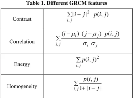
Texture feature uses the contents of GRCM to measure the variation in Gabor responses at a pixel of interest. Harlick et al. [24] first proposed in 1973, they characterize texture using a variety of quantities derived from second order image statistics. Co-occurrence texture features are extracted from an image in two steps. First, the pairwise spatial co-occurrences of pixels separated by a particular angle and distance are tabulated using GRCM approach. Second, the GRCM is used to compute a set of scalar quantities that characterize different aspects of the underlying texture. The GRCM is a tabulation of how often different combinations of Gabor responses co-occur in an image or image section Harlick et al., [24].
Table 1. Different GRCM features
Contrast i j
j i p j i , 2 ) , ( | | Correlation j
i i j
j
i j p i j
i , ) , ( ) ( ) (
Energy ij
j i p , 2 ) , (
Homogeneity i
j
i
j
j
i
p
,
1
|
|
)
,
(
4.3
kNN Classification
In supervised learning, training examples and test examples could be considered. A training example is an ordered pair hx, yi where x is an instance and y is a label. A test example
is an instance x with unknown label. The goal is to predict labels for test examples. The kNN classifier has two stages; the first is the determination of the nearest neighbors and the second is the determination of the class using those neighbors. Let us assume that there is a training dataset D made up of (xi) ϵ [1, |D|] training samples. The examples
are described by a set of features F and any numeric features have been normalized to the range [0,1]. Each training example is labeled with a class label yj ϵ Y.
Objective is to classify an unknown example q. For each xi
ϵ D can be calculated the distance between q and xi as
follows:
F
f f f if
i
w
q
x
x
q
d
(
,
))
,
(
(2)There are a large range of possibilities for the distance metric; a basic version for continuous and discrete attributes would be: continuous f x q x q d discretean x q and discrete f xi q if f if f if f f f | | 1 0 ) , (
(3)The k nearest neighbors is selected based on this distance metric. Then there are a variety of ways in which the k nearest neighbors can be used to determine the class of q. The most straightforward approach is to assign the majority class among the nearest neighbors to the query. It will often make sense to assign more weight to the nearer neighbors in deciding the class of the query. A fairly general technique to achieve this is distance weighted voting where the neighbors get to vote on the class of the query case with votes weighted by the inverse of their distance to the query.
) , ( ) , ( 1 ) ( 1 c j k
c c n
j y y
x q d y
Vote
(4)
Thus the vote assigned to class yj by neighbor xc is 1
divided by the distance to that neighbor, i.e. 1(yj, yc) returns
1 if the class labels match and 0 otherwise. The value n would normally be 1 but values greater than 1 can be used to further reduce the influence of more distant neighbors.
4.4
Decision Tress for Classification
Decision tree learning used in statistics, data mining and machine learning, uses a decision tree as a predictive model which maps observations about an item to conclusions about the item's target value. More descriptive names for such tree models are classification trees or regression trees. In these tree structures, leaves represent class labels and branches represent conjunctions of features that lead to those class labels. Decision tree learning is a method commonly used in pattern classification. The goal is to create a model that predicts the value of a target variable based on several input variables.
Four splitting rules that are widely available for growing a decision tree include: gini, class probability, twoing, and entropy. Each of the splitting rules attempts to segregate data using different approaches. The gini index is defined as:
i i ip
p
t
Gini
(
)
(
1
)
(5)
where pi is the relative frequency (determined by dividing the
total number of observations of the class by the total number of observations) of class i at node t, and node t represents any node (parent or child) at which a given split of the data is performed Apte et al[25]. The gini index is a measure of impurity for a given node that is at a maximum when all observations are equally distributed among all classes. In general terms, the gini splitting rule attempts to find the largest homogeneous category within the dataset and isolate it from the remainder of the data. Subsequent nodes are then segregated in the same manner until further divisions are not possible. An alternative measure of node impurity is the towing index:
i L R
R
L
P
P
i
t
p
i
t
P
t
Twoing
(
(|
(
|
)
(
|
)
| ))
24
)
(
(6)
where L and R refer to the left and right sides of a given split respectively, and p(i|t) is the relative frequency of class i at node t Breiman et al[26]. Twoing attempts to segregate data more evenly than the gini rule, separating whole groups of data and identifying groups that make up 50 percent of the remaining data at each successive node. Entropy, often referred to as the information rule, is a measure of homogeneity of a node and is defined as:
i i ip
p
t
Entropy
(
)
log
(7)
Where pi is the relative frequency of class i at node t Apte et
5.
EXPERIMENTAL RESULTS AND
ANALYSIS
The arecanut database contains six classes of total 2090 arecanut images. The images were taken from Canon Digital camera (Power Shot A1100IS). All the Images were taken to approximately fill the camera field of view in natural day light
with white background. Images were cropped into 32 X 32 pixel resolution to speed up computation. kNN classifier and Decision Trees have been used for classification of arecanut. The kNN classifier has given success rate of 75.64. A decision tree is used for classification, got the classification accuracy of 95.69% for Twoing rule, 95.74% for gdi and 6.31% for Entropy.
Table 2. Confusion Matrix using Decision tree classifier with Twoing splitting rule
Api Red Bette Black Bette Minne Chaali Gotu Total Success Rate in %
Api 101 0 3 0 11 2 117 86.32
Red Bette 3 90 2 0 7 0 102 88.23
Black Bette 4 2 68 1 2 0 77 88.31
Minne 0 1 0 2 3 1 7 28.57
Chaali 5 6 5 1 1677 6 1700 98.64
Gotu 11 0 1 0 13 62 87 71.26
Total 2090 95.69
Table 3. Confusion Matrix using Decision tree classifier with splitting rule Gini Diversity Index
Api Red Bette Black Bette Minne Chaali Gotu Total Success Rate in %
Api 92 3 4 0 16 2 117 78.63
Red Bette 3 91 2 0 6 0 102 89.21
Black Bette 2 3 65 0 6 1 77 84.41
Minne 0 0 1 3 2 1 7 42.85
Chaali 4 4 4 0 1682 6 1700 98.94
Gotu 8 0 0 0 11 68 87 78.16
Total 2090 95.74
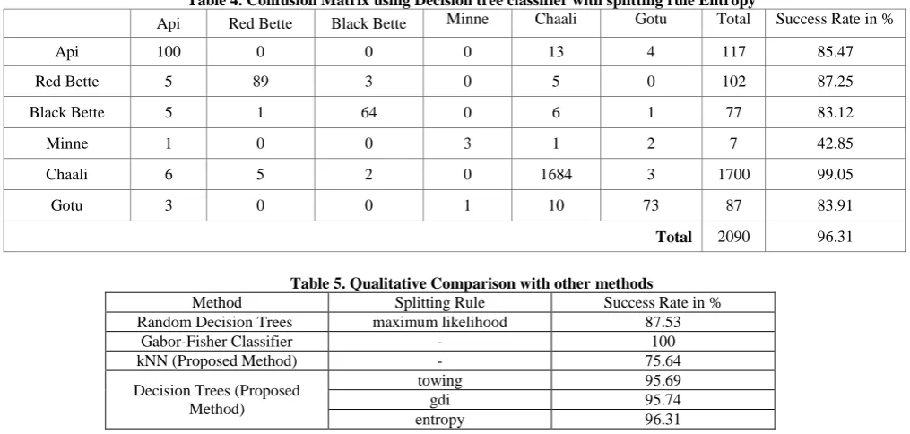
Table 4. Confusion Matrix using Decision tree classifier with splitting rule Entropy
Api Red Bette Black Bette Minne Chaali Gotu Total Success Rate in %
Api 100 0 0 0 13 4 117 85.47
Red Bette 5 89 3 0 5 0 102 87.25
Black Bette 5 1 64 0 6 1 77 83.12
Minne 1 0 0 3 1 2 7 42.85
Chaali 6 5 2 0 1684 3 1700 99.05
Gotu 3 0 0 1 10 73 87 83.91
Total 2090 96.31
Table 5. Qualitative Comparison with other methods
Method Splitting Rule Success Rate in %
Random Decision Trees maximum likelihood 87.53
Gabor-Fisher Classifier - 100
kNN (Proposed Method) - 75.64
Decision Trees (Proposed Method)
towing 95.69
gdi 95.74
Method
Figure 2: plot of success rate against different methods
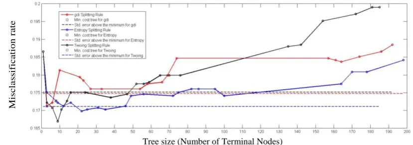
Tree size (Number of Terminal Nodes)
Figure 3: Estimated cost for each tree using cross validation
The misclassification rate against estimated cost for each tree using cross validation using Decision trees with three splitting rules gdi, entropy and twoing rule are plotted in Figure. 3. Plot reveals the behavior of feature set for each splitting rule. The splitting rule entropy demonstrated the improved success rate as 95.66%. The cost of a node is the sum of the misclassification costs of the observations in that node. The solid line shows the estimated cost for each tree size, the dashed line marks one standard error above the minimum, and the square marks the smallest tree under the dashed line. The misclassification error in entropy is less compare to gdi rule and twoing rule. Figure 2 illustrate that decision tree has given almost same success rate for all the splitting rules.
6.
CONCLUSION
In this paper, watershed segmentation has been used to segment the arecanuts images from the given images. In the segmented region GRCM features are extracted. Experimentation is conducted on GRCM features using kNN classifier and decision tree classifier. Three tree kernel functions called gdi, twoing, and entropy have been used with decision tree for analysis of results. kNN classifier has given success rate of 75.64.
With the decision tree classifier for different kernel functions, found the following observations:
twoing has given success rate of 95.69%.
gdi has given success rate of 95.74%.
entropy has given success rate of 96.31%.
An experimental result reveals that decision tree has given good success rate as compare to kNN classifier. Further, in decision tree classifier kernel function entropy has given good success rate compare to gdi and twoing rule. This method can be extended to other objects such as classification of flowers, fruits, seeds, and a vegetable etc. where there is a human intervention is in need for classification.
7.
ACKNOWLEDGMENTS
Authors would like to thank to the experts who have reviewed and given valuable suggestions.
8.
REFERENCES
[1] Nemati, R.J., Javed, M.Y. 2008. Fingerprint verification using filter-bank of Gabor and Log Gabor filters. 15th International Conference on Systems, Signals and Image Processing, 363 – 366.
[2] Lei, Yu., Yan, Ma., Zijun, Hu. 2011. Gabor Texture Information for Face Recognition Using the Generalized Gaussian Model. Sixth International Conference on Image and Graphics (ICIG), 303 – 308, 2011.
M
is
c
la
ssi
fi
c
a
ti
o
n
r
a
te
S
u
c
c
e
ss
R
a
te
i
n
[3] Chengjun, Liu., Wechsler, H. 2002. Gabor feature based classification using the enhanced fisher linear discriminant model for face recognition. IEEE Transactions on Image Processing, 467 – 476, Volume: 11 , Issue: 4.
[4] Yuanbo, Yang., Jinguang, Sun. 2010. Face Recognition Based on Gabor Feature Extraction and Fractal Coding. Third International Symposium on Electronic Commerce and Security (ISECS), 302 – 306.
[5] Foster, P. and Pedro, D. 2003. Tree induction for probability-based ranking. Journal in Machine Learning. ACM, 52(3), 199-215.
[6] Pierre, G., Damien, E. and Louis, W. 2006. Extremely randomized Trees. Machine Learning. 36(1), 3-42.
[7] Leo, Breiman., Jerome, Friedman., Charles, Stone and Richard, Olshen. 1984. Classification and Regression Trees.
[8] Ross, Quinlan. 1993. C4.5: Programs for Machine Learning. Morgan Kaufmann. San Francisco, CA, USA.
[9] Peter, F. and Edson, M. 2007. A simple lexicographic ranker and probability estimator. Proceedings of the 18th European Conference on Machine Learning (ECML 2007). 575-582, Springer.
[10] Andrew, B. 1997. The use of the area under the ROC curve in the evaluation of machine learning algorithms. Pattern Recognition. 30(7), 1145-1159.
[11] Foster, P. and Venkateswarlu, K. 1999. A survey of methods for scaling up inductive algorithms. Data Mining and Knowledge. 3(2), 131-169.
[12] Cesar, F. Peter, F. and Jose, H. 2003. Improving the AUC of probabilistic estimation trees. Proceedings of the 14th European Conference on Machine Learning. 121-132, Springer.
[13] Cristina, Olaru and Louis, W. 2003. A complete fuzzy decision tree technique. Journal Fuzzy Sets and Systems - Theme: Learning and modeling, ACM, 221 – 254.
[14] Fernando, B. Juan-Carlos, C. Nicolas, M. Daniel, S. 2004. Building multi-way decision trees with numerical attributes. International Journal of Information Sciences 165. Elsevier, 73–90.
[15] Barros., Basgalupp., de, Carvalho. Freitas. 2012. A Survey of Evolutionary Algorithms for Decision-Tree Induction. IEEE Tran. on Systems, Man, and Cybernetics Applications, 291 – 312.
[16] Moustakidis., Mallinis., Koutsias., Theocharis. and Petridis. 2012. SVM-Based Fuzzy Decision Trees for Classification of High Spatial Resolution Remote Sensing Images. IEEE Transactions on Geoscience and Remote Sensing. 149 – 169.
[17] Juan, Sun., Xi-Zhao, Wang. 2005. An initial comparison on noise resisting between crisp and fuzzy decision trees. Proceedings of International Conference on Machine Learning and Cybernetics, 2545 – 2550.
[18] Setiono, R., Huan, Liu. 1999. A connectionist approach to generating oblique decision trees. IEEE Transactions on Systems, Man, and Cybernetics, Volume: 29 , Issue:3, 440 – 444.
[19] Haiwei, Xu., Minhua, Yang. Liang, Liang. 2010. An improved random decision trees algorithm with application to land cover classification. International Conference on Geoinformatics, 1-4.
[20] Pedrycz, W., Sosnowski, Z A. 2005. C-fuzzy decision trees. IEEE Transactions on Systems, Man, and Cybernetics, Part C: Applications and Reviews. 498– 511.
[21] Crockett, K. Bandar, Z. Mclean, D. 2002. Combining multiple decision trees using fuzzy-neural inference. IEEE International Conference on Fuzzy Systems. 1523 – 1527.
[22] Rafael, C. G. and Richard, E. Woods. and Steven, L. Eddins. 2009. Digital Image Processing using MATLAB. PPH.
[23] Newsam, S. D. and Kamath, C. 2004. Retrieval using texture features in high resolution multi-spectral satellite imagery. In SPIE Conference on Data Mining and Knowledge Discovery.
[24] Harlick, R. M., Shanmugam, K., and Dinstein, I. 1973. Textural Features for image classification. IEEE Transaction on System, man and Cybernetics, 610 – 621.
[25] Apte, C. S, Weiss. 1997. Data mining with decision tress and decision rules. Future Generation Computer Systems, 13:197–210.
[26] Breiman, L. 1996. Some properties of splitting criteria. Machine Learning. 24:41–47.